Abstract
Economists and policy makers are interested in producers’ responses to policies in order to achieve some national or sectoral objectives, e.g., growth, employment, food security. The way producers respond to policy depends on their production function. If producers do not have homogenous production function, policy responses will be heterogeneous. We use the underlying functional relationship to derive homogenous groupings. The paper employs finite regression mixture models to specify and estimate farm groups with regard to pre-specified functional relationship. The proposed approach is illustrated with regard to the aggregate production function of Kosovo agriculture, characterised by high prevalence of small farmers. The results point out to two farm clusters. The first one extracts more output from labour and intermediate consumption. The second one makes a better use of land. Perhaps, surprisingly, both clusters appear quite similar in terms of their stock of production inputs. Cluster 1 however appears to be more specialised. We can conclude that in Kosovo agriculture appearances and size are not primary determinants of productivity.
1. Introduction
Economists and policy makers have always been interested in producers’ responses to policies in order to achieve some national or sectoral objectives, e.g., growth, employment, food security. The way producers respond to policy depends on their production function. The commonplace assumption that all observed units have homogenous production function leads to expectation of homogenous response [1] which is, however, not particularly realistic. If this assumption does not hold, production units’ policy responses will be heterogeneous. This heterogeneity in responses is the focus of the present paper.
Modelling heterogeneous responses has a long tradition in economics, and in particular in agricultural economics in the area of the so called ‘representative farm modelling’ [1,2]. The traditional approach splits the units of interest into relatively homogenous groups with regard to a set of pre-defined characteristics and models these separately [3,4,5]. Often the purpose of such modelling is to use the results for mathematical programming models of these different groups. The way these groups are derived can, however, be problematic. Often some form of factor analysis or principal components analysis is applied with regard to selected observable characteristics in order to identify the groups. The problem with this approach is that it yields groups which are similar with regard to the observable variables used in the analysis, but not necessarily with regard to the functional relationship which is of primary interest in such an approach.
In the present application we have an additional issue. All Kosovo farms are small. Furthermore their endowments, as demonstrated later, are quite concentrated. This means that trying to deduce different responses form differences in their characteristics would be challenging. Furthermore, one cannot safely assume that there is a dramatic difference between small-scale farms and the rest, when the rest is virtually non-existent. Hence, while in may CEECs countries a well-defined dualistic farming structure (with a large number of small farms and a very small number of larger ones) provides a natural differentiation in which smallholders coexists with large production units his is not the case in Kosovo. It could be tempting to assume that all small farms are to some extent similar, since they have similar characteristics. Yet, such an assumption would only hold if their response to production incentives is fully defined by their characteristics. Such an assumptions is, however, entirely baseless since it essentially is equivalent to assuming that production functions (the production response) only depend on farming characteristics. The production function, however, is a function of these characteristics and hence such an assumption is equivalent to saying that all farms share the same production function. In this paper we invert the question and ask: given the observed production response, how many qualitatively different production functions are necessary to describe the farming population.
We propose to specify homogeneous groups with regard to the pre-specified functional relationship, in this case a production function. The groups are estimated using finite regression mixture models. We propose this method as the most adequate when the issue in hand is either to investigate policy responses of groups of firms (farms) with similar production function, or to model their production function in a follow-up simulation model. The empirical analysis is focused on the aggregate agriculture production relationship. It provides a farm classification based on the production function which, in contrast to the farm characteristics generally used in the clustering approach, is not directly observable. Examining such a classification for a specific country has distinct policy implications. Different groups of farms, identified using the proposed methodology, are expected to react differently to production incentives and to shock as the most recent COVID-19 and the war in Ukraine, as well as to policy attempts to smooth these shocks, since by definition they have different production functions. Although still there is not systematic farm level management data on the impact of the above shocks, the study in this paper will provide insights to policy-makers whether they should expect harmonized or differentiated response by smallholders to their policy incentives to smooth the consequences of these unexpected shocks. The aggregate reaction of the agricultural sector will be a weighted average of the responses of the different groups.
The proposed approach is illustrated with regard to the aggregate production function of Kosovo agriculture. Kosovo is chosen as a case study since the interest in this paper is on smallholders. Kosovo is one of the poorest countries in Europe. Table 1 compares Kosovo with the other Western Balkan countries, the European Union (EU) and the countries of Europe and Central Asia, excluding the high income ones [6]. The data indicates that Kosovo is consistently the poorest country. Compared to the EU (Kosovo contemplates to join the Union and formally applied for membership in 2022), GDP per capita in Kosovo in purchasing power parity is within the range of one fifth to one fourth of the value in the EU.

Table 1.
GDP per capita, Purchasing Power Parity (constant 2017 international dollars).
In line with the other countries in the Western Balkans, agriculture is an important sector in Kosovo [7]. Kosovo share of agriculture, forestry and fisheries in the GDP in the period 2012–2020 varied between 7–8% (Table 2), while in the EU it was between 1.6 and 1.7% [6]. Kosovo’s agriculture is characterised by serious structural problems. These include land fragmentation, low labour efficiency and high production costs [3]. The majority of farms are very small in physical size. According to the Agricultural Household Survey, carried out by the Kosovo Agency of Statistics, in 2018 there were 108,108 agricultural holdings with total land area of 185,130 ha. In terms of land area, the largest proportion (i.e., 74%) constituted smaller holdings with less than 2 ha, while only 1.7% were holdings larger than 10 ha [7,8].
Table 2.
Agriculture, forestry, and fishing, value added (% of GDP).
Despite these structural problems, Kosovo agriculture faced by the unexpected COVID-19 shock has been resilient. For example, if the non-food retail trade shrunk, the turnover of food retail in spring 2020 increased in comparison to 2019 [9]. Apart from increasing demand, since people stored food at home, two other factors boosted the resilience of the agricultural sector. First, by the time COVID-19 started farmers had managed to purchase their inputs. Second, the government introduced several measures to support agriculture, e.g., increased subsidies on some perishable products and doubled (as one-off) the amount of direct payments on a range of eligible crop and livestock products [10,11]. Therefore, a stable food demand accompanied by boosted agricultural policy support allowed Kosovo farming sector to adjust to the shock of the pandemic. However, the negative consequences for small farmers, focus of the present paper, have been more exacerbated than could be revealed by the overall agricultural performance. For some period of time they were out of their traditional marketing channels, i.e., local open air markets which were closed during the pandemic. Only large supermarket chains were allowed to continue trading but small farmers were not integrated in the supermarkets’ value chains.
The results from our analysis point out to two farm clusters in Kosovo. What is striking in the obtained classification is that these two groups appear very similar with regard to production factors, with exception of capital. Yet, the two groups make very different use of their endowments in terms of the amount of output they manage to extract from each of these production factors. A more detailed characterisation of the differences between the two groups shows that the more productive group appears to be more specialised in a variety of ways.
2. Motivation
In this section the authors are motivated to propose a novel methodology. The reasons for this choice are presented hereafter. Economic theory has a longstanding tradition of emphasising uniformity. The principle of the ‘representative economic agent’ is probably the best known theoretical abstraction in economics. Assuming such uniformity is very useful in deriving theoretical properties helping microeconomic models to be easily expressed into common sense logic. This approach has been very fruitful in producing logical outcomes based on sound principles of rationality. Furthermore, it has also provided a basis for statistical investigation. Since this concept is an abstraction and it is obtained by averaging the reactions of the actual economic agents, the representative agent responses can be obtained by averaging the observed responses of the actual agents. Hence, although directly unobservable, estimating a mean regression type of statistical model implicitly yields the response of the representative economic agent.
This uniformity principle, although useful, has its limitations and has been questioned. From a theoretical point of view, models of bounded rationality which combine two types of representative agents have been shown to be able to produce qualitatively different outcomes. For example, [12] present a model with rational agents and noise traders who behave randomly and interact with the rational agents. One of the surprising outcomes of this model is that the noise traders, who non-intentionally (i.e., randomly) make very risky investments, may under certain conditions end up dominating the market. [13] further investigate this issue, which is now accepted in financial literature [14,15].
The use of typologies is aimed at somewhat relaxing the uniformity principle by accounting for farm heterogeneity. However, the purpose of establishing such typologies is not descriptive, but rather functional [16].
Clusters describing farmer typologies are often created with the intention to derive implications for some policy design [17] or market responses [18]. The idea is that accounting for inherent heterogeneity allows for better aggregation of farm-level responses. For this purpose however individual farm-level responses need to be coherently aggregated [16] in order to obtain reliable results for policy adjustments. To differentiate driving effects, the use of farm types as a consolidated model is particularly helpful [19]. In order to be able to achieve such a coherent aggregation we need two preconditions: first, the groups (types) need to be representative with regard to the desired (i.e., investigated) reaction function and second, we need to be able to identify the relative shares of these types, so that appropriate weighting for aggregating the heterogeneous responses can be established
In this paper, however, we are not concerned with the theoretical challenges to the uniformity principle, but rather with some empirical considerations. A major problem in empirical research is that the theory rarely prescribes the form of the functional relationship between the variables in question. It is essentially not possible to know beforehand the functional form of this relationship. Hence, the problem of ‘representativeness’, i.e., homogeneity in response, becomes intertwined with the issue of the functional specification. There is a clear trade-off in this area. Using more flexible functional representation reduces this problem, but also makes the interpretation and inference more difficult, and in some cases impossible (as in the case of the curse of dimensionality problem). Using more restrictive functional representations results in more tractable models, but in this case the representativeness assumption is more likely to be violated simply because the used functional representation is inadequate. Therefore, the representativeness condition in empirical modelling is dependent on a given functional specification. In other words, the question of whether the units of analysis exhibit the same relationship is only meaningful with regard to the given functional form of this relationship.
To simplify the issue, the following discussion focuses on the production function, but our argument is equally applicable to other functional relationships. Grouping units of analysis with regard to their production function (or any other functional relationship of interest), we propose in this paper, not only asks the relevant question (i.e., what different functional relationships describe the data) directly, but also makes the classification issue explicitly dependent on the choice of the functional form. It provides a clear definition of the kind of representativeness the researcher is looking at. If the aim is to group farms with similar production function either because this is the characteristic of interest or because the intention is to model their production function in a follow-on simulation model, this is clearly the question that has to be asked. A clustering type of approach, in contrast, asks a very different question. It asks how similar the units appear to be with regard to some predefined observable characteristics. Such a question leaves the issue of ‘representativeness’ very vague. In contrast to this in many empirical clustering applications the choice of cluster building components such as fusion algorithms or distance measures is not explicitly dependent on the purpose of such classification meaning that the results can impose a certain structure rather than reveal one [20]. The clustering approach also implicitly claims a kind of logically inconsistent universality. For example, one may use some set of ‘relevant variables’ to cluster units and then assume that the functional relationship is homogeneous within each cluster. However, the same approach could be applied to a wide range of relationships, such as, e.g., cost, profit and production functions. Therefore, the units in the same cluster are assumed to have the same type of functional relationship for all of the above. This is an unrealistic assumption.
Finally, there is another more practical consideration. Economic analysis is often based, as in this paper, on aggregate relationships, which undoubtedly contain unobserved heterogeneity. For example, when one looks at the issue of production function, since technologies are very different for different farm typologies, it is reasonable to consider different production functions for different types of farming typologies, e.g., livestock, crop, vegetables, etc. farms. Yet, doing so, results in a large number of underlying models without actually solving the problem of unobserved heterogeneity, since even within a certain typology different technologies could co-exists, based on characteristics that are not directly observable. Therefore, from a purely practical point of view, there is a trade-off: on the one hand, one would want a small number of functional relationships, but on the other, would want these relationships to encompass both the similarities and differences amongst the units of interest, in this case farms. In other words, subject to the constraints defined by the choice of functional relationship, one wants the best combination of such functional relationships that describes the data. Hence, in our application of the proposed method of classification the main question becomes: how many distinct production functions can describe the output response of Kosovo agriculture and what are their characteristics? In this way, one not only provides a characterisation of an economic sector (agriculture), but also simultaneously determines the behaviour of its production units.
Whenever the policies do not affect the structure of agriculture, i.e., they do not affect the balance (i.e., the weights) of the different groups, the proposed methodology will just provide an approximation to that response (i.e., production function). However, useful such an approximation might be, there are alternatives that can achieve the same result (e.g., using a more flexible functional form). The real advantage is apparent when policies have structural effects and they affect the balance of the classified groups. In this case, the structural change effects can be inferred by examining the differential production responses by different groups.
3. Materials and Methods
We employ finite regression mixture model to specify and estimate farm groups with regard to the pre-specified production function. It is assumed that, conditional on a set of covariates X, y arises from a probability distribution with the following density:
where pk are the mixing proportions (0< pk <1 for all k and ), and probability distribution, parameterised by . This means that y can be viewed as drawn from K different underlying (conditional) probability distributions. The parameters specify a regression model, i.e., they include regression coefficients, as well as the distribution parameters. In this study, we use a linear regression specification [21,22], but in principle any other parametric specification, could be used instead. The nature of the estimation algorithm is very general and allows for a wide range of specifications. Equation (1) states that the data-generating process for y, conditional on X, is a mixture of regressions. Thus, if y is the output and X are the inputs, this expression states that the data comes from several distinct production functions.
One can obtain the maximum likelihood estimate for the parameters by using the Expectation Maximisation (EM) algorithm of [23] and then apply the ‘maximum a posteriori’ (MAP) principle to assign observations to each of the underlying distributions. The EM algorithm we used in the analysis consists of the following two steps, namely, the E(xpectation) step and the M(aximisation) step. In the E step the conditional probability of observation i belonging to during the m-th iteration for all i and k, is given by:
where the bracketed superscripts denote estimates for the parameters during the corresponding iteration.
In the M step the ML estimate, of , is updated using the conditional probabilities, , as conditional mixing weights. This leads to maximizing:
The updated expressions for the mixing proportions are given by:
The updating of depends on the parametric specification and, therefore, no general formula can be given. The maximisation step is essentially the standard maximisation routine used to estimate the conditional model given some fixed, determined in the expectation step, mixing proportions. The generic Equation (3) expresses calculating the log-likelihoods for each separate component and maximising the weighed likelihood with weights given by the posterior probabilities . Thus, by adapting the maximisation step, a wide range of models could be fitted.
The above description assumes that one knows the exact number of clusters. However, this is typically not the case. Choosing the appropriate number of mixing distributions (clusters) is essentially a model selection problem. One can estimate the regression mixture models for different number of clusters and then selects amongst these. A popular criterion in model selection problems is the Bayesian Information Criterion (BIC) defined as:
where m is any model (thus m denotes the choice of the parametric (conditional) distributions g(.) or any combination thereof), K is the number of components, L is the (maximised) complete log-likelihood and v is the number of free parameters in the model and n is the sample size. If the choice of g(.) is taken for granted, then (5) suggests a strategy of consecutive estimation of (m, K) models for K = 1, 2, … until BIC increases. The consecutive estimation strategy also ensures against the danger of over-fitting the statistical model.
BICmK = −2 Lmk + vmKln(n)
The BIC is based on an asymptotic approximation of the integrated log-likelihood valid under some regularity conditions. It has been proven that the BIC is consistent and efficient on practical grounds [24]. Moreover, the whole class of penalised likelihood estimators, of which the BIC is a special class, are consistent [25,26]. The BIC is furthermore approximately equivalent to the popular in information theory Minimum Description Length (MDL) criterion [27]
In order to select a model where in addition to the model fit the ability to define well separated clusters is taken into account, the integrated complete likelihood (ICL) criterion can be used. According to [16], the ICL can be expressed as BIC with an additional entropy penalty term as follows:
where are the cluster membership indicators. In the present application, one is explicitly interested in the degree of separation of clusters. Hence, the ICL will be used.
The finite regression mixture approach describes the functional relationship as a hierarchical mixture model, where the data generation process generates each observation from a finite set of underlying sub-models, which define separate clusters. As explained in the motivation section, these clusters represent different functional relationships (i.e., different production functions). Hence, the representativeness condition is defined directly with regard to the production function conditional on its functional form. An advantage of the finite mixture approach is the ease by which data observations can be attached to the different underlying production functions.
4. Data and Choice of Functional Form
As explained, the approach to specify homogenous groups of observations based on underlying functional relationship is applied empirically to farms in Kosovo. Empirical estimations are based on data from the Kosovo version of the Farm Accountancy Data Network (FADN) for 2016 [28]. It follows the EU’s FADN which monitors farms’ income and business activities and provides microeconomic management data based on harmonised questionnaire and national surveys of farmers [29,30]. Funded by the European Agency for Reconstruction, in 2005 a pilot FADN project started in Kosovo with a survey of 50 farms. This network was expanded to 159 farms in 2006, continuing, with an increase in the number of holdings to 300 in 2008 and 394 in 2013 and 2014 [28]. In 2011, as a legal basis setting the criteria for inclusion of farms in FADN and the identification of the annual farm income, an administrative instruction was approved. Until 2012, data was collected by advisory services but since 2013 a specialised company was contracted to collect data in different regions of Kosovo.
A qualitative improvement in Kosovo FADN coverage has taken place since 2016 when a new sample was designed based on the results from Agriculture Census 2014. Agriculture holdings have been classified based on the type of farming and economic size. The sample units of FADN observation covered 54% of total number of agriculture holdings, 91.6% of total standard output, 86.6% of total UAA and 89.3% of total LSU. The data cover information on the farm, land use, production and assets, marketing activities and subsidies [28]. This improved FADN sample is used in this paper.
In the empirical specification the farm output is specified as a function of four inputs, namely capital, labour, land and intermediate consumption (IC). These are the standard production factors in agricultural production routinely employed in production function estimations [31].
Summary statistics for the data are presented in Table 3. Labour is measured in Annual Work Units (AWU) and Land in hectares (ha), while all other variables are in monetary terms, namely in euros. Relatively small farms manage to pass the FADN inclusion threshold, which in Kosovo is low in comparison to other EU Member States in order to reflect the nature of Kosovo farms structure (2000 EUR Standard Output). There seems to be considerable heterogeneity in terms of all variables amongst the farms included in the dataset. Since the mean values for all variables are closer to the minimum than the maximum values, there are more relatively smaller farming units and a very long right tail representing the smaller number of larger farms in the distribution for all considered variables. This distributional feature is not particularly surprising, but any such heterogeneity suggests that the functional relationships amongst these variables may also be heterogeneous. In particular, the considerable differences in terms of size that are evident in the data set could lend themselves to differences in the production relationship, since it is not unreasonable to expect that as farms grow larger, the organisation of their activities changes and therefore the input/output relationship might change too.
Table 3.
Summary statistics.
The key question in the paper is whether the Kosovo farms can be described by the same production function. As already discussed, this question requires specifying the inputs and the functional form for the specific production function. There is extensive literature on the issue of production functions, and their theoretical and empirical properties [32,33,34]. With regard to the problem in hand, it is advisable to employ a production function specification that is sufficiently flexible, since in a finite regression modelling framework there is a clear trade-off between flexibility and the potential number of homogenous groups, i.e., more flexible functional forms will reduce the number of groups. Here, we employ the translog functional specification.
In the production function literature the term ‘flexible’ has a specific meaning. According to [35], a functional form can be denoted as ‘flexible’ if its shape is only restricted by theoretical consistency. The translog functional specification can be restricted to satisfy the homotheticity, homogeneity or separability, but in this application no such restrictions have been applied. The main reason for this is that by avoiding restrictions one can maintain its generality. Furthermore, as our previous argument demonstrates, there is a clear trade-off between flexibility and the potential number of clusters since flexible specifications would result in a smaller number of clusters. Therefore, since the question is whether a single production function specification is sufficient to describe the data, it makes sense to avoid imposing restrictions that could inflate the potential number of clusters.
Although in more recent studies the translog appears to have somewhat fallen out of favour with empirical researchers, it is still the most extensively investigated second order flexible functional form and surely the one with the most empirical applications as its empirical applicability in terms of statistical significance is outstanding [36,37]. Furthermore, the fact that the translog function can be considered as a second order (Taylor series) approximation of a more general production function provides a sound justification in applying it here, since the uncertainty about the production function is a major justification for the present study.
An important reason for the choice of the translog specification is also that it is linear with regard to the parameters, which means that standard linear regression techniques can be used for estimation and testing purposes. In principle, estimating a finite regression model simply requires plugging in the M step an estimation routine for the underlying model, which creates tremendous flexibility since this means that the underlying model can be fully nonparametric. Linear specifications offer considerable savings in terms of computational costs.
5. Results
The model fitting ICL criterion indicates that a single common translog production function is not sufficient to describe the Kosovo farms and points out to two clusters (Figure 1). Furthermore, since ICL accounts for both model fit and cluster separation, this demonstrates that these two clusters are well separated. In practical terms, this means that at least some of the corresponding coefficients are significantly different, resulting in two quite different production functions, subject to the functional restriction of a translog functional form.
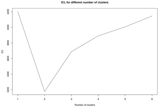
Figure 1.
ICL determination of number of clusters.
Table 4 presents some summary statistics for the two clusters. Cluster 1 is considerably smaller with only 144 farms while Cluster 2 contains 1044 farms. In terms of the variables used in the production function, however, there do not appear to be major differences between the two clusters. With exception of capital, where Cluster 2 has more on average and maybe intermediate consumption where it is the other way round, the clusters look very similar in that respect. Since the standard deviations for all variables are smaller in Cluster 1 one may say that it is more compact (in the sense that it exhibits more internal similarity) than Cluster 2. In order to formally check the above propositions, we carried out several tests and their p-values are presented in the second part of Table 2. The standard t-test for equality in the means is insignificant except for capital implying that only the capital endowments of the two clusters are different. The other two tests – the Kolmogornov-Smirnov (KS) and the Mann–Whitney U-test (which is essentially a two-sample version of the Wilcoxon test) are more general tests for difference in the distributions. As expected, both these are significant for capital (since the cluster means are different, distributions will clearly differ), but they fail to detect any distributional difference for any other factor of production or indeed output. Hence, we can conclude that the two clusters only differ in terms of their capital endowments.
Table 4.
Clusters summary and separation.
Yet, our estimation suggests that in spite of looking very similar, the two clusters have very different production functions. Due to the non-linear functional form of these, however, comparing estimated coefficients would be impractical and non-informative. A reliable way to compare two non-linear functions is by comparing their partial correlation plots. This amounts to using the estimated models to predict the dependent variable (i.e., output) and then plot the predicted values against the values for a given factor by keeping the other factors fixed at ‘typical’ values. In this way, we can visualize the effect of a given production factor when the rest of the inputs are kept fixed. The first issue is what would be the reasonable values for the fixed inputs. This would depend on the purpose of the above plot. If the interest is in average effects, using the average values over the estimation sample would be an easy way to achieve ‘reasonable values’. Sometimes averaging would not be a reasonable strategy, in particular in the case of discrete values (see, e.g., [31]). In the present study, all the inputs are continuous variables, therefore, averaging over the estimation sample is used as a viable option.
The second issue concerns the need to create a prediction sample containing a range of values for the input variable of interest, create the relevant (transformed) variables needed in the translog specification and predict from the estimated linear model. The only choice necessary is the range of values for the analysed input. We have employed a regular grid of 100 points defined over the range within which the input in question is observed. Since the two clusters are potentially different in their input mixes, it is reasonable to produce separate ranges for each cluster. In this way, the values for the variable of interest are actually observable within the estimation sample. The resulting plots show the range of values for each input by cluster and this facilitates the interpretation of the results. It also avoids the danger of predicting outside the range over which each of the two clusters is defined. As for the variables over which any such plot is conditioned upon (i.e., the other inputs), averaging over the whole sample is applied in order to ensure that the effects plotted for the two clusters are comparable. Since the summary statistics for both clusters exhibit considerable dispersion, it is easy to verify that such common ‘typical’ values lie comfortably within the range of observable values for each of the two clusters and, therefore, the synthetic observations created in order to produce the effects of interest are feasible.
Plotting the effects for each input can provide a useful overview of the differences between the corresponding production functions. However, the usefulness of such a comparison would be limited without information on how different statistically these are, which requires confidence intervals for such effects that can be obtained by bootstrapping the corresponding models. Here, we used the nonparametric case bootstrap, following [25].
The partial correlation plots for the inputs are presented in Figure 2, Figure 3, Figure 4 and Figure 5. Both output and the inputs have been transformed back into the original units in order to facilitate a meaningful interpretation. Due to the non-linear nature of the model, the confidence intervals are asymmetric. The differences in the production relationships are quite striking. Cluster 1 manages to extract more output from labour and intermediate consumption, while Cluster 2 makes more productive use of land. Since the effects are only plotted over the effective range of values for the corresponding inputs, it can be seen that the maximum values for both labour and land (as well as capital) are smaller in Cluster 1. The capital effects only show a tentative picture in that they suggest that Cluster 1 might be able to make a better use of its smaller stock of capital. However, since the confidence intervals for the capital effect in Cluster 1 are quite wide, statistically such a difference cannot be established.
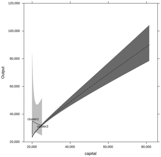
Figure 2.
Capital effects by cluster.
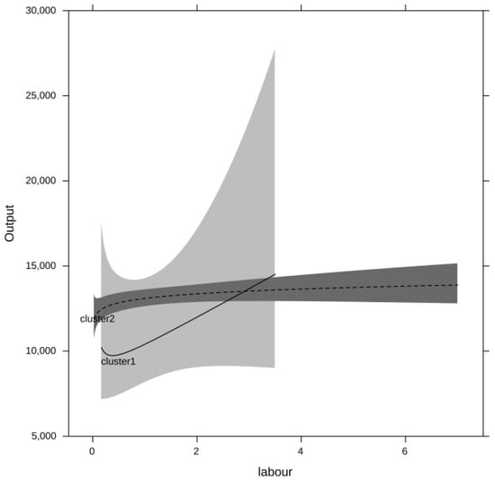
Figure 3.
Labour effects by cluster.
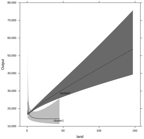
Figure 4.
Land effects by cluster.
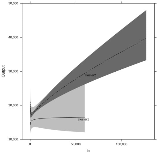
Figure 5.
Intermediate consumption effects by cluster.
Furthermore, the partial correlation plots demonstrate a clear differentiation between the two clusters in that the corresponding confidence intervals rarely overlap reinforcing the conclusion that their production functions are markedly different.
Given the similarity of the two clusters and the startling difference in their respective production functions, an important question is about the source of this difference. One of the possible explanations is that these clusters differ in terms of other unobservable, with regard to the empirical approach adopted in this paper, characteristics. Additionally, while some clustering based on a set of such characteristics could always be an option in empirical analysis, it is clear that by modifying the set of such characteristics one may end up with different characterisations, while the approach we adopted here produces unique with regard to the assumed functional relationship groupings. Yet, it would be informative to test whether the two cluster differ with regard to such unobservable characteristics. Another potential source of such difference could be the different types of land use by farms. Cultivating, e.g., different crops, imposes different requirements for labour and capital, as well as different configuration of intermediate consumption. Instead of looking at the multitude of such possible land use configurations, we employed a single measure of the distribution of land use. Three specific measures are applied, i.e., Shanon (entropy) diversity index, richness and the equitability index. The Shannon index is where is the land area share allocated to the ith land use, while the equitability is defined as E = S/Max (S). The equitability index is a standardised Shannon index (divided by its maximum value, so that it fits the [0,1] interval). The richness is simply the number of separate land uses found on a farm.
In simple terms, the above three measures capture the extent to which land use is concentrated or more evenly spread amongst different types of uses. The idea is that more specialised farms will be characterised by a lower values across all these measures. Furthermore, the distribution for any of the above measures will reflect the extent of multiple land use within the farms and, hence, by comparing the corresponding distributions one should be able to reflect on the difference in the two clusters. Unfortunately, the Kosovo FADN only provides a rough classification of land use consisting on 12 different types of use. It does not, for example, distinguish between the different types of cereals. However, this is probably sufficient for our purposes since crops within the same group (e.g., oilseeds or cereals) typically have similar production technologies.
Table 5 presents some summary statistics concerning the distribution of these measures within each of the two clusters. In particular, the table presents the overall range minimum and maximum, alongside the empirical quartiles and the means for each cluster. A look at these summaries suggests that the values for all such statistics is typically larger for Cluster 2, hinting that Cluster 1 may be more specialised, which could explain its higher productivity. To check this conjecture, we tested tor difference in means and distribution, as before (in Table 2). All these tests, with exception of the (non-parametric) Mann- Whitney U-test for equitablity index, suggest that the underlying distributions are indeed different. One can therefore confirm that Cluster 1 is more specialised than Cluster 2.
Table 5.
Land use differences between the clusters.
6. Conclusions
In this paper we used finite regression mixture models, based on an underlying relationship of interest for classification of heterogeneous units of analysis. We applied the proposed approach to Kosovo farms production function.
The results suggest that there are at least two clusters with distinct production functions. While these two clusters appear to be similar in terms of their aggregate inputs, they have very different production functions. Cluster 1 is much smaller in terms of number of farms but manages to extract considerably more output from most inputs with the exception of land, whilst Cluster 2 is more productive. What is particularly interesting is that while being similar in many respect, the one difference between the two clusters is the capital endowments since Cluster 2 has much more capital. Yet, in contrast to conventional thinking, more capital does not extend to higher productivity. In fact, it is Cluster 1 which manages to make more productive use of its inputs. The main reason for this differential productivity performance appears to be the higher level of specialisation of Cluster 1.
It would be useful to consider how such production system might respond to external shocks. The general economic shocks could be expected to increase unemployment implying more labour supply to agriculture. This would benefit Cluster 1 which extracts more output from labour. Yet, this is the smaller (in terms of number of farms ) cluster. Hence, the positive labour effects would be somewhat limited. Cluster 2 has higher absorption capacity for the extra labour. It extracts more output from land, which is in restricted supply, meaning that land is essential for allocating the surplus labour. As we have discussed, Cluster 2 is also more diversified in terms of different uses for its land. Such a diversification is an expected livelihoods supporting strategy. It could therefore be expected that crises and external shocks would lead to relative growth of Cluster 2. Yet, the production potential is clearly in Cluster 1. This suggests that agricultural policies should be more focused on enabling the growth of this particular cluster.
The analysis in the paper has several limitations which we intend to deal with in future work on small farmers. The proposed approach is explicitly conditioned on a predefined functional relationship. Re-appraising the latter in both functional form or additional characteristics of interest would allow one to better tune the empirical application with a more focused research context. Furthermore, although the present application used a cross-sectional data, it is straightforward to extend to a longitudinal data contexts, where a more detailed insight could be obtained.
An external constraint we faced is that the collection and finalization of FADN data normally takes several years before the network is ready for analysis and could be accessed. Our data precedes the external shocks of COVID-19 and the war in Ukraine. We would like to repeat this study with more recent data which will allow to see the impact on small farmers and their adjustment process. Such an analysis calls for a longitudinal study.
Author Contributions
Conceptualization, P.K. and S.D.; methodology, P.K.; software, P.K.; validation, P.K. and S.D.; formal analysis, P.K. and S.D.; investigation, P.K. and S.D. All authors have read and agreed to the published version of the manuscript.
Funding
This research received no external funding.
Institutional Review Board Statement
Not applicable.
Data Availability Statement
The data used in this study belongs to the Kosovo government. The portion of data used in this analysis would be made available to interested researchers upon request.
Conflicts of Interest
The authors declare no conflict of interest.
References
- Köbrich, C.; Rehman, T.; Khan, M. Typification of farming systems for constructing representative farm models: Two illustrations of the application of multi-variate analyses in Chile and Pakistan. Agric. Syst. 2003, 76, 141–157. [Google Scholar] [CrossRef]
- Robertson, M.; Pannell, D.; Chalak, M. Whole-farm models: A review of recent approaches. AFBM J. 2012, 9, 13–25. [Google Scholar]
- Tittonell, P.; Vanlauwe, B.; de Ridder, N.; Giller, K.E. Heterogeneity of crop productivity and resource use efficiency within smallholder Kenyan farms: Soil fertility gradients or management intensity gradients. Agric. Syst. 2007, 94, 376–390. [Google Scholar] [CrossRef]
- Briggeman, B.C.; Gray, A.W.; Morehart, M.J.; Baker, T.G.; Wilson, C.A. A new US farm household typology: Implications for agricultural policy. Rev. Agric. Econ. 2007, 29, 765–782. [Google Scholar] [CrossRef]
- Bidogeza, J.C.; Berentsen, P.B.M.; de Graaff, J.; Lansink, A.G.J.M.O. A typology of farm households for the Umutara Province in Rwanda. Food Sec. 2009, 1, 321–335. [Google Scholar] [CrossRef]
- World Bank World Development Indicators, Series: Agriculture, Forestry, and Fishing, World Bank; Washington DC. Available online: https://datatopics.worldbank.org/world-development-indicators/ (accessed on 4 December 2022).
- MAFRD (Ministry of Agriculture, Forestry and Rural Development). In Prishtina, Kosovo Green Report 2020; MAFRD: Pristina, Kosovo; Available online: https://www.mbpzhr-ks.net/repository/docs/Green_Report_2020r.pdf (accessed on 4 December 2022).
- DEAAS (Department of Economic Analysis and Agricultural Statistics). Kosovo Agriculture in Numbers; DEAAS: Pristina, Kosovo, 2021. [Google Scholar]
- GAVFSP (Good Agriculture and Food Security Programme). From Farmers to Financial Institutions, the Impacts of COVID-19 in Kosovo are Widespread, JUL. 08, 2020|IMPACT STORIES, GAEVFSP, Wahington, DC. 2020. Available online: https://www.gafspfund.org/news/farmers-financial-institutions-impacts-covid-19-kosovo-are-widespread (accessed on 4 December 2022).
- Hyseni, B. The Impact of COVID-19 on Agriculture, Food And Rural Areas in Kosovo. In Proceedings of the Agricultural Policy Forum 2020, 13 October 2020; Available online: https://apf.seerural.org/wp-content/uploads/2020/10/10.-WG1-KOSOVO_The-impact-of-COVID-19-Basri-Hyseni.pdf (accessed on 4 December 2022).
- MAFRD (Ministry of Agriculture, Forestry and Rural Development). Kosovo Green Report, 2018; MAFRD: Prishtina, Kosovo, 2018. [Google Scholar]
- De Long, J.B.; Shleifer, A.; Summers, L.H.; Waldmann, R.J. Noise trader risk in financial markets. J. Political Econ. 1990, 98, 703–738. [Google Scholar] [CrossRef]
- Kogan, L.; Ross, S.; Wang, J.; Westerfield, M. The price impact and survival of irrational traders. J. Financ. 2006, 61, 195–229. [Google Scholar] [CrossRef]
- Cogley, T.; Sargent, T.J. Diverse Beliefs, Survival and the Market Price of Risk. Econ J. 2009, 119, 354–376. [Google Scholar] [CrossRef]
- LeBaron, B. Heterogeneous gain learning and the dynamics of asset prices. J. Econ. Behav. Organ. 2012, 83, 424–445. [Google Scholar] [CrossRef]
- Luo, G.Y. Conservative traders, natural selection and market efficiency. J. Econ. Theory 2012, 147, 310–335. [Google Scholar] [CrossRef]
- Moro, D.; Sckokai, P. The impact of decoupled payments on farm choices: Conceptual and methodological challenges. Food Policy 2013, 41, 28–38. [Google Scholar] [CrossRef]
- Andersen, E.; Elbersen, B.; Godeschalk, F.; Verhoog, D. Farm management indicators and farm typologies as a basis for assessments in a changing policy environment. J. Environ. Manag. 2007, 82, 353–362. [Google Scholar] [CrossRef] [PubMed]
- Weltin, M.; Zasada, I.; Franke, C.; Piorr, A.; Raggi, M.; Viaggi, D. Analysing behavioural differences of farm households: An example of income diversification strategies based on European farm survey data. Land Use Policy 2017, 62, 172–184. [Google Scholar] [CrossRef]
- Huynh, T.H.; Franke, C.; Piorr, A.; Lange, A.; Zasada, I. Target groups of rural development policies: Development of a survey-based farm typology for analysing self-perception statements of farmers. Outlook Agric. 2014, 43, 75–83. [Google Scholar]
- Dolnicar, S. A Review of Unquestioned Standards in Using Cluster Analysis for Data-driven Market Segmentation. Working Paper Series, Faculty of Commerce, University of Wollongong, Wollongong, Australia, 2002. [Google Scholar]
- De Sarbo, W.S.; Cron, W.L. A maximum likelihood methodology for clusterwise linear regression. J. Classif. 1988, 5, 249–282. [Google Scholar] [CrossRef]
- Wedel, M.; Kamakura, W.A. Market Segmentation—Conceptual and Methodological Foundations, 2nd ed.; International Series in Quantitative Marketing 2001; Kluwer Academic Publishers: Boston, MA, USA, 2001. [Google Scholar]
- Dempster, A.P.; Laird, N.M.; Rubin, D.B. Maximum likelihood from incomplete data via the EM algorithm. J. R. Stat. Soc. Ser. B 1977, 39, 1–22. [Google Scholar]
- Fraley, C.; Raftery, A. Model-Based Clustering, Discriminant Analysis, and Density Estimation. J. Am. Stat. Assoc. 2002, 97, 611–631. [Google Scholar] [CrossRef]
- Keribin, C. Consistent estimation of the order of mixture models. Sankhya Ser. A 2000, 62, 49–66. [Google Scholar]
- Biernacki, C.; Celeux, G.; Govaert, G. Assessing a mixture model for clustering with and integrated completed likelihood. IEEE Trans. Pattern Anal. Mach. Intell. 2002, 22, 719–725. [Google Scholar] [CrossRef]
- Hastie, T.; Tibshirani, R.; Friedman, J. The Elements of Statistical Learning: Data Mining, Inference, and Prediction, 2nd ed.; Springer Series in Statistics; Springer: New York, NY, USA, 2016. [Google Scholar]
- MAFRD. Kosovo FADN Implementation, Department of Economic Analysis and Statistics; MAFRD: Pristina, Kosovo, 2018. [Google Scholar]
- Delforge-Delbrouck, A. FADN Methodology A to Z; European Commission: Brussels, Belgium, 2020. [Google Scholar]
- European Commission. Agriculture and Rural Development, Farm Accountancy Data Network at a Glance. EU, Brussels. Available online: https://agriculture.ec.europa.eu/data-and-analysis/farm-structures-and-economics/fadn_en (accessed on 4 December 2022).
- Kostov, P.; Davidova, S.; Bailey, A. Effect of family labour on output of farms in selected EU Member States: A non-parametric quantile regression approach. Eur. Rev. Agric. Econ. 2018, 45, 367–395. [Google Scholar] [CrossRef]
- Bridge, J.L.; Griliches, Z.; Ringstad, V. Economies of Scale and the Production Function. Econ J. 1972, 82, 766–768. [Google Scholar] [CrossRef]
- Berndt, E.R.; Christensen, L.R. The translog function and the substitution of equipment, structures, and labor in U.S. manufacturing 1929–68. J. Econom. 1973, 1, 81–113. [Google Scholar] [CrossRef]
- Christensen, L.R.; Jorgenson, D.W.; Lau, L.J. Transcendental logarithmic utility functions. Am. Econ. Rev. 1975, 65, 367–383. [Google Scholar]
- Diewert, E.W. Functional Forms for Revenue and Factor Requirements. Int. Econ. Rev. 1974, 15, 119–130. [Google Scholar] [CrossRef]
- Feger, F. A Behavioural Model of the German Compound Feed Industry: Functional Form, Flexibility, and Regularity. Ph.D. Thesis, Georg-August Universität, Göttingen, Germany, 2000. [Google Scholar]


Disclaimer/Publisher’s Note: The statements, opinions and data contained in all publications are solely those of the individual author(s) and contributor(s) and not of MDPI and/or the editor(s). MDPI and/or the editor(s) disclaim responsibility for any injury to people or property resulting from any ideas, methods, instructions or products referred to in the content. |
© 2023 by the authors. Licensee MDPI, Basel, Switzerland. This article is an open access article distributed under the terms and conditions of the Creative Commons Attribution (CC BY) license (https://creativecommons.org/licenses/by/4.0/).