Optimization Model of Permanent Basic Farmland Indicators Distribution from the Perspective of Equity: A Case from W County, China

Abstract

Based on its national conditions and food availability, China has embarked on the road to establishing food security in a way by implementing the concepts of innovative, coordinated, green, open and inclusive development, and the requirements of high-quality development and a national food security strategy for a new era. As a result, the permanent basic farmland protection zone designated for high-quality arable land reserves had become a fundamental national policy. However, the allocation of permanent basic farmland protection quantity indicator is always a challenge due to the conflicts between the development and protection process. The unequal protection indicator allocation is often cited as an inefficient source of permanent basic farmland production and protection. In this article, an optimization model is introduced to allocate preservation indicators by using the Gini coefficient, a widely used index of income inequality in economics. The optimization model is based on a hierarchical structure of the multi-criteria factors and the objective weighting method. The allocation of a permanent basic farmland protection indicator in W county, China, is chosen as a case study to illustrate the application of this model with a focus on a balance between equality and efficiency. The result shows that the method can provide profound insight for land management policymakers.

1. Introduction

In recent years, the world has been undergoing rapid urbanization. The more rapid the accelerated urbanization process is, the more serious the decline in cultivated land is in the region [1,2]. In the 1960s, the United States, Japan and other countries put forward the scientific demarcation and guarantee system of important agricultural land to deal with a series of problems such as the pressure of urban expansion, environmental damage and food security. In the United States, important farmland was divided into basic farmland, special farmland, state important farmland and local important farmland [3]. In 1967, Japan formulated the Law on Territorial Readiness of Agricultural Development to establish a nationwide “agricultural development zone”, thus ensuring the development of agricultural zones and the effective use of farmland. Subsequently, the Land Use Plan Law was enacted in 1974 and the National Land Use Plan was promulgated in 1976. These two laws and regulations clearly defined the relationship between agricultural land and non-agricultural land [4]. At the same time, the law also made it clear that agricultural land designated as basic farmland must be concentrated and contiguous. In the 1980s, China began to pay attention to the quantity of farmland, and the land system focusing on farmland protection was constantly emerging. In 1986, the Land Administration Law was promulgated, laying the foundation for the comprehensive establishment of the basic farmland protection system [5]. In 1994, Mr. Lester Brown, director of the Worldwatch Institute, published a study named “Who will feed the Chinese?”. This article aroused people in China to think about population problem and food security [6]. In 1998, the revised Regulations on the Protection of Basic Farmland stipulated that basic farmland was cultivated land that could not be occupied according to the general land use plan for a certain period of time [7]. According to legal and institutional requirements, the Chinese government had implemented an overall plan for land use throughout the country. It draws a red line for 120 million hectares of cultivated land [8]. It strictly controls the occupation of cultivated land, especially high-quality land which is called permanent basic farmland. Compared with cultivated land, permanent basic farmland has a more prominent status, stricter protections, a more stable spatial pattern, and a more important position and role in stabilizing food production. Most importantly, permanent basic farmland cannot be used for construction unless approved by the higher government after a strict and long procedure.

In order to ensure the amount of permanent basic farmland, the central government divided this task to local governments through administrative orders, which only need to meet the indicator quantity requirements [9]. Although some simple guidelines were given in the legislation, the distribution process was more in accordance with the administrative orders and less operational due to the lack of quantitative standards and a scientifical framework [10]. Thus, the tension between the pressure to provide land for economic growth and the imperative to preserve permanent basic farmland was played out at all levels of local government. Therefore, how to reasonably decompose the indicators of permanent basic farmland can help coordinate the relationship between development and protection, and promote better protection of cultivated land. In 2018, the Chinese government began a new round of territorial spatial planning at the national level [11]. At present, a new round of territorial spatial planning is being compiled. Facing 2035, the plan will lay the overall pattern of China’s land and space development in the next 15 years. At the same time, how the indicators decompose was always the core content in spatial planning. In summary, the research on this issue had a certain reference significance for the preparation and study of territorial spatial planning.

Meanwhile, since the reform and opening up, China’s economy has continued to grow. The income of residents has increased significantly, and the society as a whole is in a harmonious and orderly state. However, the unfair distribution among regions and industries has become increasingly prominent. Low-efficiency, negative-efficiency and even pseudo-efficiency growth modes still existed. The 13th National Congress of the Communist Party of China put forward that “social equity should be reflected on the premise of improving efficiency”. Nowadays, promoting fairness has increasingly become the principle of China’s social modernization governance. Therefore, indicators distribution was not only a technical issue, but also a social management matter in China. Because the distribution area of cultivated land often overlaps with the suitable area for urban construction, the delineation of permanent basic farmland would limit the expansion of construction land. The unequal distribution was often cited as a source of inefficiency in permanent basic farmland production and protection [12]. Therefore, the decomposing of a permanent basic farmland preservation indicator was not only a crucial element regarding productivity issues in agriculture, but also had significantly equal consequences for regional development and rural employment, maintenance of rural landscapes, biodiversity and the protection of the environment.

In this research, a hierarchical structure of multi-criteria factors was proposed, which allocated the permanent basic farmland preservation indicator by using the Gini coefficient optimization model. A case study of allocating a preservation indicator for W county, China, in 2025, is provided to illustrate the application of this indicator decomposing model.

2. Literature Review

Many researchers have focused on the model of permanent basic farmland indicators distribution. Scientific evaluation systems and analysis methods were introduced into the model. At first, some single-level models based on agricultural production factors began to be built to quantify the role of those decisive elements, such as agriculture quality, agriculture production infrastructure and natural conditions [13]. Then, multiple indicators began to introduced into the models. Yang et al. [14] selected indicators from site conditions, agricultural production and transportation locations, and constructed a multiple indicators evaluation system, and delineated permanent basic farmland based on the comprehensive score. Combined with semi-quantitative analysis, Chen et al. [15] decomposed the basic farmland index of Jiangxi Province by considering the current situation, the planned amount of cultivated land, the supply conditions of basic farmland and the protection index assigned to the region by higher authorities. Bao combined the spatial analysis functions and site assessment method to establish an evaluation index system [16]. Screening medium and high-yield fields, cultivated land area and cultivated land infrastructure condition factors, Zhao et al. [17] established a decomposition model of cultivated land protection index by taking villages as a unit. Liu et al. [18] used an analytic hierarchy process combined with spatial autocorrelation analysis of basic farmland to determine the index weights. Most of the comprehensive considerations have been based on the natural conditions, economic benefits and utilization levels of cultivated land [19]. Since the 21st century, spatial analysis software has been more and more widely used in the optimization of basic farmland. The main idea for spatial optimization of permanent basic farmland was to comprehensively determine the distribution and indicators of permanent basic farmland based on farmland suitability evaluation and other restrictive conditions [20]. There were also scholars who demarcate permanent basic farmland by calculating the productivity of cultivated land based on the results of agricultural land quality classification [21]. Some scholars also used model methods, such as the XGS decision model [22], CLUE-S model [23], LESA model [24], etc. The above studies have improved the scientificity of the distribution of permanent basic farmland. However, most of the weighting of indicators still had a certain degree of subjectivity, which caused some confusion to solve the multi-objective optimization problem.

The permanent basic farmland preservation has received continuous attention from many perspectives. Nevertheless, less attention had been directed towards the allocation from equality insight. Regarding fair evaluation, most scholars usually use the evaluation index of equal distribution, such as the Gini coefficient, theil index and coefficient of variation [25]. Among them, the Gini coefficient is a measure of statistical dispersion. It has features that make it useful as a measure of dispersion in a population and inequalities in particular [26]. It is a ratio analysis method, making it easier to interpret. Thus, the Gini coefficient is widely used in many fields. For example, in ecology, the Gini coefficient has been used as a measure of biodiversity, where the cumulative proportion of species was plotted against cumulative proportion of individuals. In education, it has been used as a measure of the inequality of universities. Consequently, the research on the decomposing of permanent basic farmland preservation indicators has been developed from the Gini coefficient model.

3. Study Area

The study area called W county is located within the Yangtze River Delta near the southeast coast of China (Figure 1B,C). The W county covers 1245 km² and has 16 towns, with flat terrain and well-developed water system suitable for agricultural production. Nowadays, it is the place with the fastest urbanization in China, which is an important county to support in the urban strategic transformation in southern Jiangsu. To its east is Shanghai, the biggest city in China. Hence, the urban-rural land use structure of this area is complicated and rapidly changing. As a result, this area becomes an ideal laboratory for the research on farmland protection and development. In this article, the 16 towns affiliated with W county would be the research unit. According to the spatial distribution pattern of each township in W county (Figure 1A), the 16 towns are divided into three spatial segments: East, middle and west. Among them, the eastern plate is adjacent to Wuxi, which is a concentrated area of heavy industry in W county. The central segment closely surrounds the main urban area of Changzhou City. The urbanization level of this region is relatively high, and the level of economic and social development is ahead of other towns, including Nanhutang, Niutang, Yaoguan, Nanxiashu and Xihu town. The urbanization level of the western plate is relatively low, and the planting industry is developed. This division is not only a spatial division, but also closely related to the economic and social development characteristics of each town. The land use data comes from the annual land use change survey data from local Land and Resources Bureau. Social and economic data comes from the W county Social and Economic Statistical Yearbook [27]. Planning materials (online open version) were collected by our research team.

4. Methodology

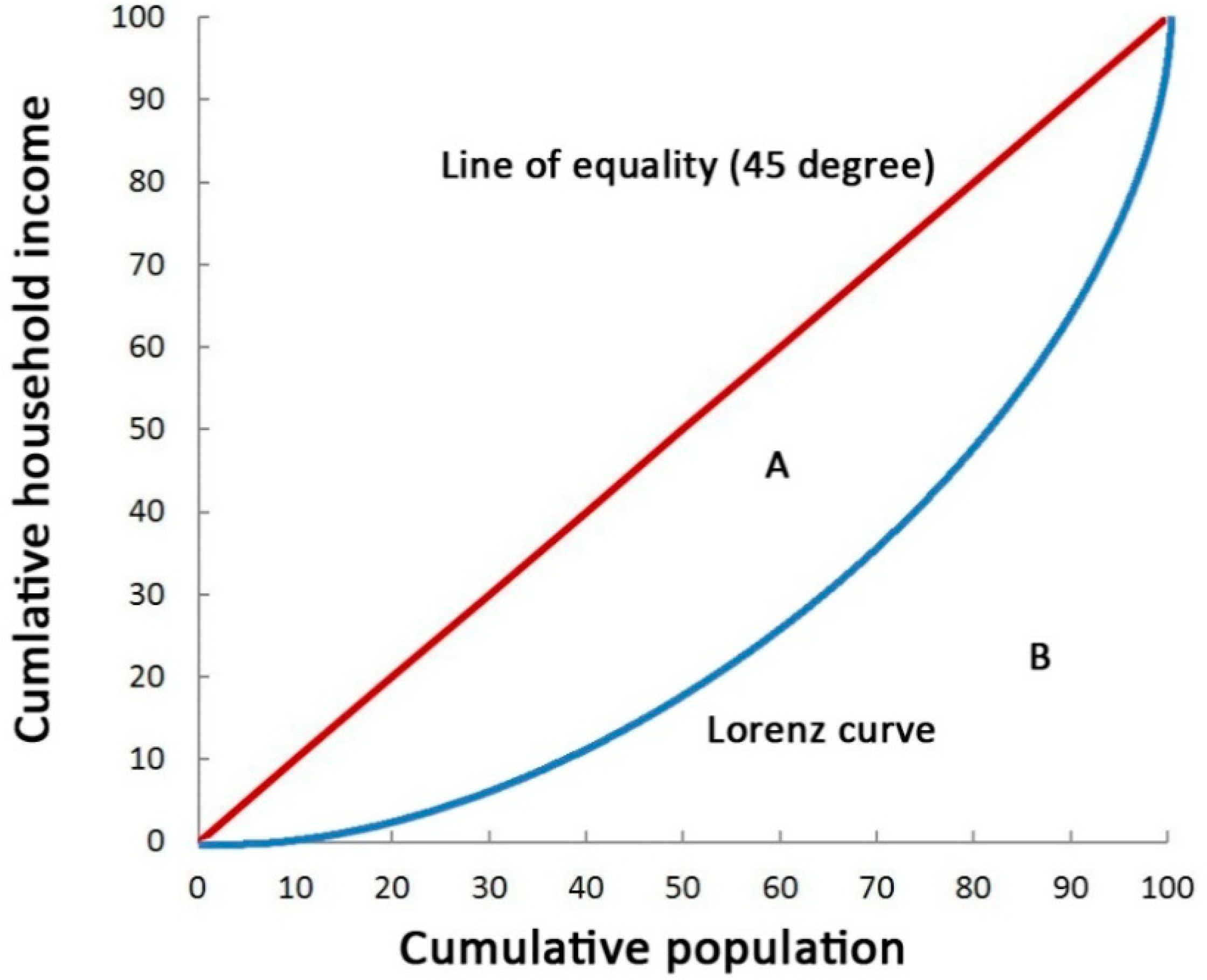
4.1. Gini Coefficient Method

The Gini coefficient is a measure of statistical dispersion developed by the Italian statistician and sociologist Corrado Gini and published in his 1912 paper “Variability and Mutability”. The Gini coefficient is usually defined mathematically based on the Lorenz curve, which plots the proportion of the total income of the population (y-axis) that is cumulatively earned by the bottom x% of the population (Figure 2). The line at 45 degrees thus represents perfect equality of incomes. The Gini coefficient can then be regarded as the ratio of the area that lies between the line of equality and the Lorenz curve (marked A in the diagram) over the total area under the line of equality (marked A and B in the diagram). The Gini coefficient is calculated by G = A/(A + B). The Gini coefficient can theoretically range from 0 to 1. A society that scores 0.0 on the Gini scale has perfect equality in income distribution. The larger the number is over 0, the higher the inequality is.

The Gini index is defined as a ratio of the areas on the Lorenz curve diagram. If the Lorenz curve is approximated on each interval as a line between consecutive points, then area B can be approximated with trapezoids.

$$G_{ini}=1-{\displaystyle \sum _{i=1}^n(X_i-X_{i-1})(Y_i+Y_{i-1})}$$

(1)

X_i is the cumulated proportion of the population variable, for i = 0,...,n, with X₀ = 0.

Y_i is the cumulated proportion of the income variable, for i = 0,...,n, with Y₀ = 0.

4.2. Coefficient of Variation Method

The coefficient of variation method is an objective weighting method. This method refers to giving different weights for assessment factors according to the degree of difference between the values of various indicators. For a set of data X₁, X₂, …, X_m, its coefficient of variation as follows:

$${\delta }_j=\frac{S_j}{\overline{x_j}}(\mathrm{Standard}\mathrm{Deviation}:S_j=\sqrt{\frac{1}{m}{\displaystyle \sum _{i=1}^m{\left(x_{ij}-\overline{x_j}\right)}^2}},\mathrm{Mean}\overline{x_j}=\frac{1}{m}{\displaystyle \sum _{i=1}^m{x}_{ij}})$$

(2)

If ${\delta }_j$ is the coefficient of variation of indicator No. j (j = 1, 2, ...n) at this time, the corresponding weight of this indicator can be expressed as:

$$W_j=\frac{{\delta }_j}{{\displaystyle \sum _{j=1}^m{\delta }_j}}$$

(3)

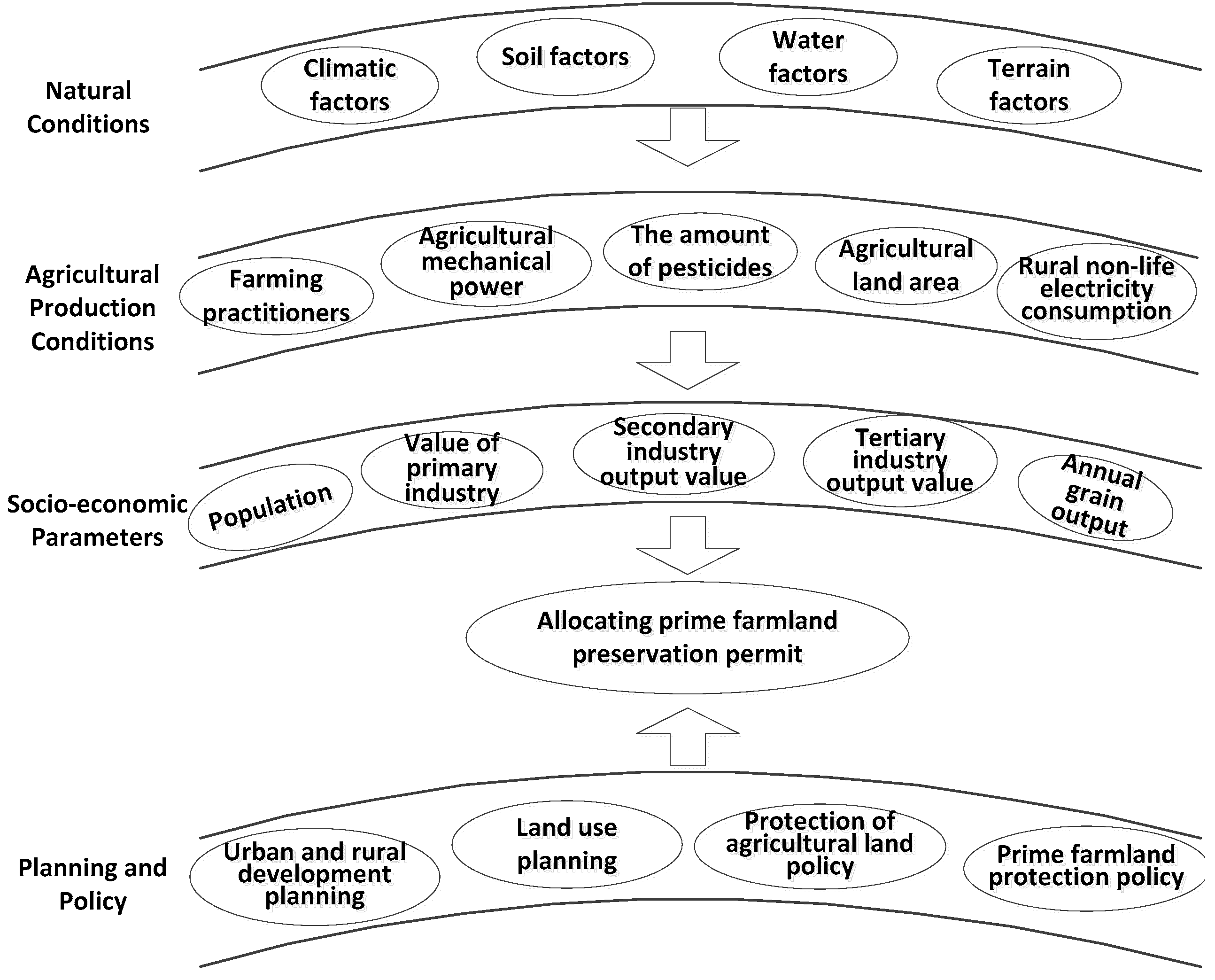
4.3. Hierarchical Structure of the Impact Factors

The premise of applying the impact factor analysis method in proper practice was to understand it correctly [28]. Factors of land use distribution had been treated as stand-in-line (single-level) factors but had not been recognized as forming a hierarchical structure in the past. According to the above related research, this study has taken full consideration of principal impact factors, to establish a complete evaluation parameter framework. By adopting an overall point of view, the parameter framework was divided into natural conditions, agricultural production conditions, social economic indicators and planning policy factors. The distribution of permanent basic farmland preservation was directly related to the natural conditions in each town. Behaviors of the farm cultivation were influenced by agricultural production conditions, such as labor, local organizations, fertilizing machines and so on. Furthermore, both the farm labor and the local organizations were influenced by government policy and a variety of land-use regulations. In this way, the factors at each level were as follows:

(1)

Factors of natural conditions: permanent basic farmland indicator distribution was greatly affected by natural conditions; climate, topography, soil and water-use conditions were necessary. The agricultural land classification and gradation had been quickly calculated based on the above natural conditions data. The quality of agricultural land in W county was classified with the grading. Meanwhile, the grading score was published and renewed regularly. In this analysis, the achievements of agricultural land classification in 2018 would be taken into account. The grading scores in 16 research units were represented as composite factors of natural conditions.

(2)

Factors of agricultural production conditions: Factors such as farming practitioners, power of agricultural machinery, consumption of pesticide, family labor and nonliving electricity affected the efficiency of farmland production. Most factors of agricultural production conditions were considered in this analysis.

(3)

Factors of social and economic conditions: Factors in this level include many external conditions affecting farmland production and protection. The population of secondary and tertiary industry (the population in

Table 1. The change of G ini coefficient of each assessment index.

Index	Gini Coefficients			Weight of Parameter
	Before Optimization	After Optimization	Decrease Proportion (%)
Population	0.31	0.279	10.135	0.057
Value of primary industry	0.246	0.246	0.000	0.132
Value of non-primary industry	0.486	0.471	3.110	0.088
Employees in planting	0.255	0.246	3.406	0.148
Total grain yield	0.393	0.348	11.464	0.132
Total power of agricultural machinery	0.265	0.236	10.889	0.103
Consumption of pesticide	0.259	0.237	8.290	0.092
Nonliving electricity consumed in rural areas	0.546	0.546	0.000	0.127
Agriculture land	0.062	0.017	72.597	0.087
Natural conditions	0.305	0.288	5.444	0.010
Planning and policy factors	0.266	0.249	6.327	0.025
Gross coefficients	0.318	0.298	6.232	1.000

) represented the development degree of labor markets which was also an indirect source of labor and consumption capacity of agricultural products in each town. Similarly, the GDP factor has been divided into two evaluation factors: the primary industry value and the non-primary industry value. The output value of primary industry and annual grain yield have shown the agricultural productive capacity in each research unit. The output value of secondary and tertiary industry represents the development degree of the industrial economy, which can provide equipment guarantee and technological innovation for agricultural production. It was also the basis to measure the modernization degree of agricultural production in towns.

(4)

Planning and policy factors: The agricultural development policy of local administration, forces of urbanization and the planning of urban-suburban land use were all included in this group. In addition to land use planning indicators, the quantitative indicators of policy factors mainly included the last round of farmland protection indicators and the number of consolidation and reclamation projects, which should serve as an important potential source of permanent basic farmland. It was also the embodiment of the agricultural development policies of towns in terms of indicators.

With a single-level model, we cannot grasp such mechanisms of effects adequately [29]. Here, the factors prescribing permanent basic farmland preservation indicator distribution form a hierarchical structure as shown in Figure 3.

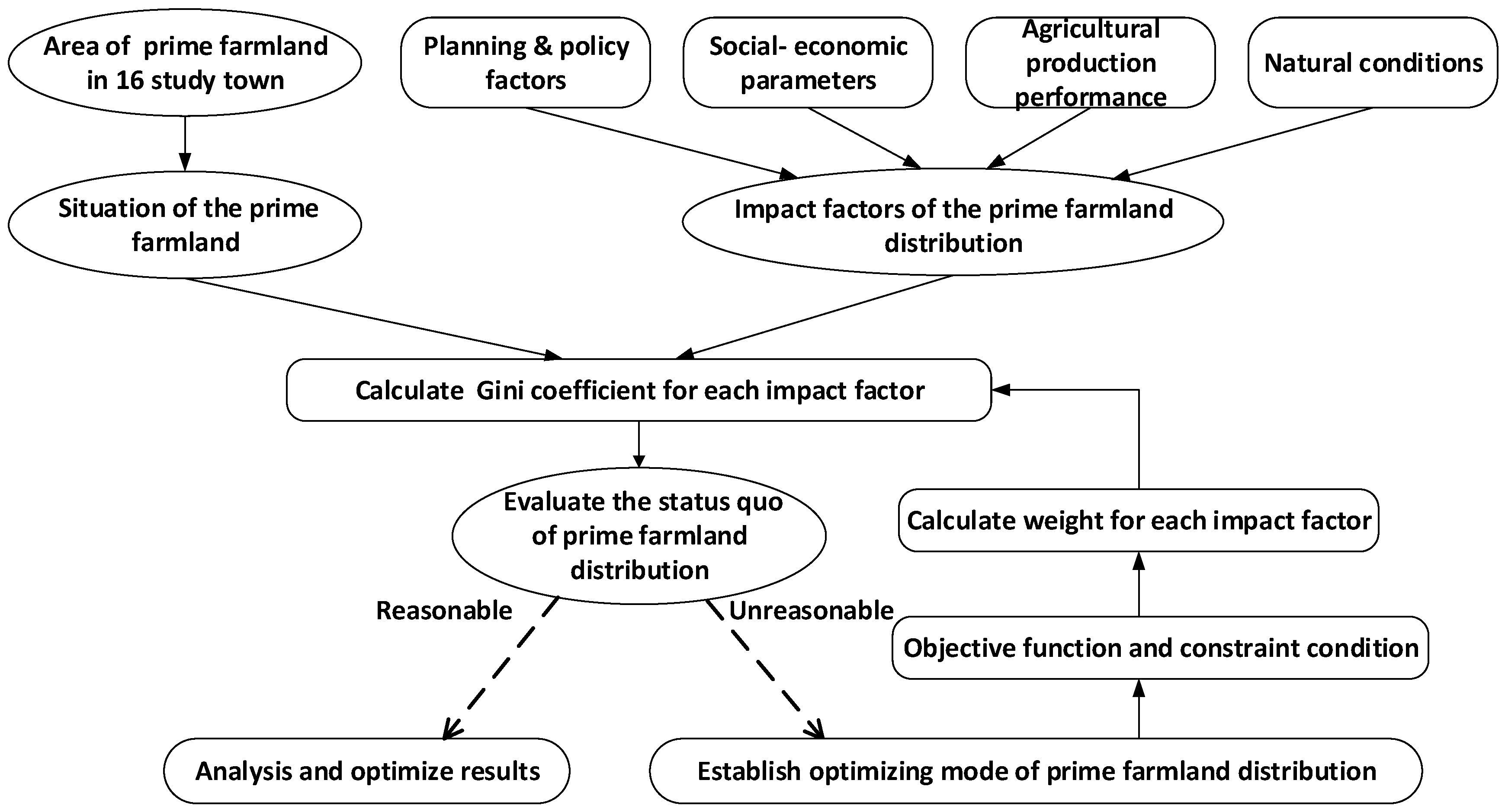
4.4. Allocation Steps

Calculate the permanent basic farmland distribution Gini coefficient corresponding to various impact factors and their weight. Evaluate whether the status quo of permanent basic farmland distribution was fair and reasonable; if not, establish the optimizing mode of the indicator distribution, which can be used to work out a reasonable distribution program. In the end, the result should be analyzed and optimized. The technology route map of this research can be seen in Figure 4.

The optimizing model of the permanent basic farmland layout based on the Gini coefficient was established according to the optimal planning method in operational research.

$$\mathrm{Target}\mathrm{Function}:\min G={\displaystyle \sum _{j=1}^m{W}_{\mathrm{j}}}{G}_j$$

(4)

$$st.\{\begin{array}{l}0\le {\mathrm{G}}_j\le {\mathrm{G}}_{0j}\\ G_{0j}\le 0.4\\ {\mathrm{Y}}_{0j}\le {\mathrm{Y}}_i\le G_{uj}\\ {\displaystyle \sum _{i=1}^n{\mathrm{Y}}_i=40803}\end{array}$$

In this formula, G represents the comprehensive Gini coefficient. W_j represents the weight of parameter j. G_0j represents the Gini coefficient of parameter j before the optimization (j = 1, 2…, 9). y_i represents the Indicator of the permanent basic farmland in each unit after the optimization. y_0i represents the lower limit of the preservation indicator in each research unit, whereas y_ui represents upper limit (i = 1, 2…, 16).

4.5. Constraints and Calculations

To ensure the fairness of the preservation target distribution, the comprehensive Gini coefficient of parameters should be as close to zero as possible. As a result, the target function was the minimum sum of the Gini coefficient weight of each parameter. In addition, according to related regulation and policy, the optimizing mode sets 3 constraint conditions.

(1)

In order to ensure the fairness of the permanent basic farmland layout, the Gini coefficient after the optimization should be no bigger than G_0j. The Gini coefficient after the optimization should be smaller than the warning value of 0.4. This warning value had been regarded as the segmentation line of the fair distribution [24].

(2)

Referring to the practice of balance between occupation and compensation of local cultivated land, the land type composition of permanent basic farmland consists of two processes: static demarcation and dynamic compensation. At present, a new round of demarcation of “three districts and three lines” in China is being carried out. Due to the limitation of data sources, this study adopted the classification standard of the second land resources survey. The lower limit (y_0i) of the permanent basic farmland preservation indicator in each research unit was 0.8 times of the current farmland area. Meanwhile, the upper limit (y_ui) of the permanent basic farmland area was the sum of the existing farmland area and 0.5 times of the garden plot.

(3)

According to the permanent basic farmland protection planning of W county, the total area of permanent basic farmland in the research zone will reach 40,803 hm² in 2025. Therefore, this study takes this value as the final binding condition.

5. Result

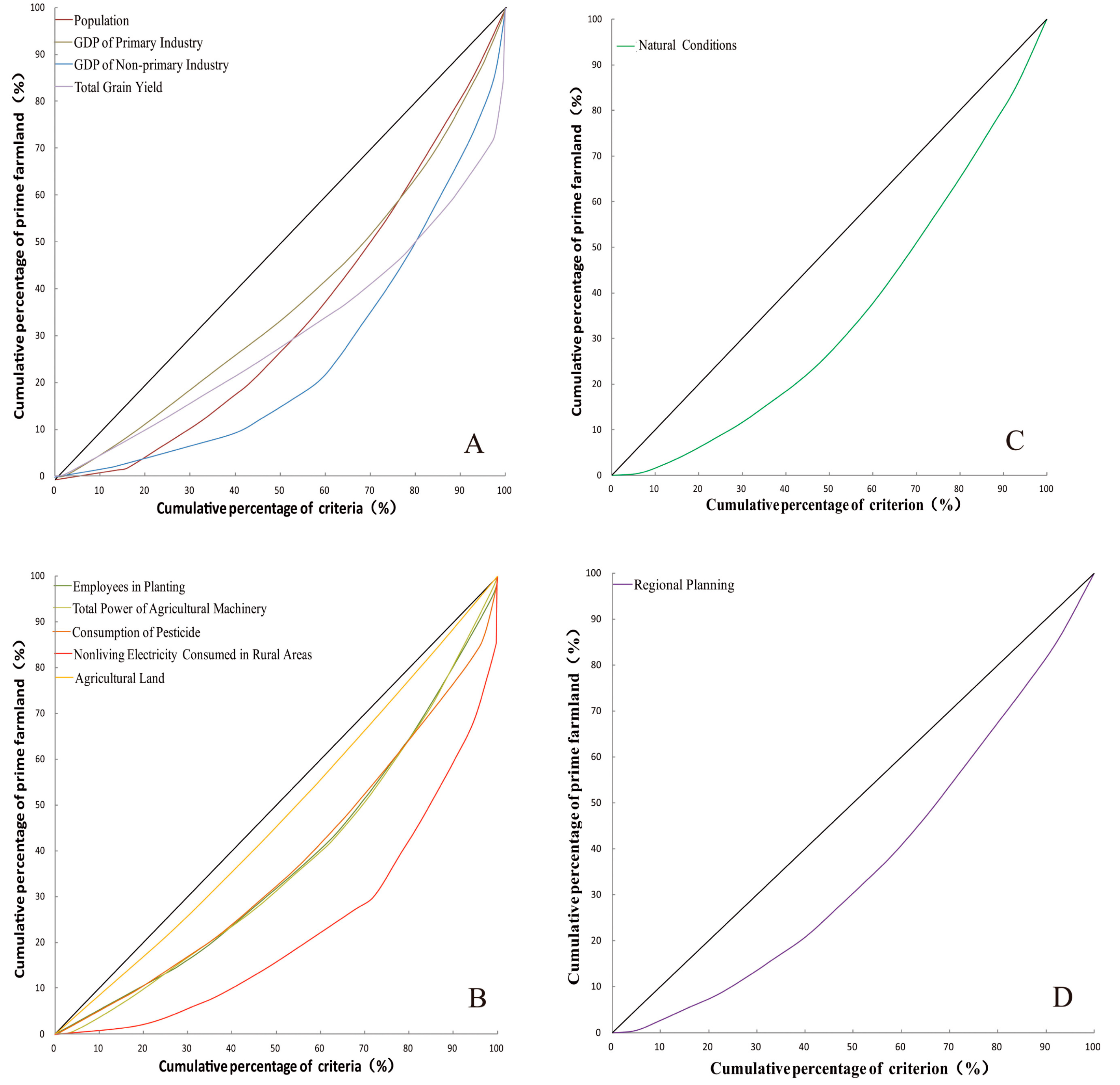
5.1. Lorenz Curve Based on Each Assessment Index

The 16 towns in W county were regarded as the 16 units. The indicator of permanent basic farmland in each town was regarded as object optimized. The ratios of these impact factors to the permanent basic farmland area were sorted in ascending order. Calculate the cumulative percent of each impact factor and then draw the corresponding Lorenz curve (Figure 5). Afterwards, calculate the Gini coefficient of each impact factor to permanent basic farmland area according to Formula (3).

According to Figure 5 and

Table 2. Comparison of permanent basic farmland indicators between the before and after optimizing.

Town Area	Indicators of Permanent Basic Farmland (Units: Hectare)
	Before Optimization	After Optimization	Value of Increase and Decrease	Coefficient of Increase and Decrease (%)
Huangli	4366	3493	−873	−20.00
Zouqu	3732	2986	−746	−20.00
Henlin	1372	1098	−274	−20.00
Jiaze	6117	5056	−1060	−17.34
Hutang	867	739	−127	−14.72
Benniu	2887	2754	−132	−4.59
Qianhuang	4356	4435	78	1.81
Yaoguan	1118	1146	28	2.55
Nanxiashu	1874	1923	48	2.59
Lijia	2751	2869	117	4.28
Hengshanqiao	1874	1954	80	4.30
Zhenglu	3638	3860	221	6.09
Niutang	1351	1439	88	6.52
Luoyang	2120	2358	237	11.22
Xueyan	3940	4429	488	12.40
Xihu	205	257	52	25.36
Total	42,576	40,803

Remark: “−” means the area of agriculture land decreased and the other means the area increased.

, the two groups of the Gini coefficient, namely the output value of non-primary industry and nonliving electricity consumed in rural areas, was on a highly average level. The Gini coefficient of the population, farming employee population and pesticide amount was on a relatively average level. The Gini coefficients of secondary and tertiary industry and the agricultural diesel oil consumption had a relatively big difference. The Gini coefficient of the rural non-living electricity consumption to permanent basic farmland area was on a level of an extremely big gap. As a result, it was necessary to adjust the permanent basic farmland indicator in each town according to the optimization mode to ensure the fairness of the indicator in 16 units.

5.2. Final Allocations after Optimizing

The weight of each impact factor according to Formula (3) was calculated to obtaint the permanent basic farmland indicators (Table 2) based on fairness and the Gini coefficients of various impact factors after optimization. From Table 2, we can see that the permanent basic farmland which needs adjusting in each research unit of W county can be clarified into four aspects: the permanent basic farmland indicator drastically decreasing area (−20~−15%); the permanent basic farmland indicator slightly decreasing area (−15~0); the permanent basic farmland indicator slightly increasing area (0~10%); and the permanent basic farmland indicator drastically increasing area (10~26%).

6. Discussion

6.1. Gini Coefficient of Final Allocation

The Gini coefficient of each evaluation index was obtained after feedback optimization by the Gini coefficients method. The Gini coefficient of final allocation shows that:

(1)

After optimization, Table 1 shows that the gross Gini coefficient had decreased from 0.318 to 0.298. Meanwhile, all the Gini coefficients of the impact factors were lower than the warning value of 0.4 after the optimization, which showed that the optimization program was reasonable.

(2)

The Gini coefficient of all indicators was not lower than the warning value, which related to the existing amount of cultivated land and the allowable increase or decrease in each town. If these factors were not taken into account, radical fair schemes would be of great harm to economic development and social management. On the other hand, this was related to the objective function of the optimization model, which only required the weighted sum of Gini coefficients of all indexes to be minimum, but did not require that Gini coefficients of all indexes be lower than the warning value. Therefore, this scheme was to obtain the optimal solution under the constraint conditions. On the premise of fairness, the index allocation was more operational than before. Because the central government still had a minimum quantity limit for the management of permanent basic farmland, it was not required that every parameter be lower than the warning value to pursue ultimate fairness such as in other studies [30].

(3)

To some extent, the lower Gini coefficients of agriculture land represented the weaker influence of agriculture land on the allocation of permanent basic farmland. On the contrary, the influence of some factors had not declined although the coefficient is reduced. Most weights of agricultural production conditions factors were larger, such as farming practitioners, power of agricultural machinery, consumption of pesticide, family labor and nonliving electricity. Those factors affected the efficiency of farmland production. Therefore, the impact of production efficiency on cultivated land protection should play a greater and greater role. Thus, changing the original only considers farmland itself as a single factor, which is consistent with the view of Zhang et al. [31]. With this hierarchical structure model, we could grasp such mechanism of effects adequately.

(4)

Indicator weight setting is the key to solving a multi-objective optimization problem. However, the selection of indicator weights still has a certain degree of subjectivity in some of the relevant literature [32,33]. In this study, the objective weight of each index had been set according to the coefficient of variation method, all of which makes the result more reasonable, avoiding the difference in subjective scoring results.

6.2. Analysis of Allocation Results

Considering the natural conditions, socio-economic factors, agricultural production factors and planning policy, the rapid development of a social economy leads to high demand for development right. For a region with a high economic development level, the higher cost of land acquisition will lead to the incline of permanent basic farmland to a low-speed development area, which was consistent with the view of Zhang et al. [34].

(1)

The permanent basic farmland drastically decreasing areas include Huangli, Zouqu, Henlin and Jiaze town. From Figure 1, we can see that these areas were mostly located in the northwest of the research area. These towns have thousands of years of continuous agricultural product history. Although the permanent basic farmland area occupied a prodigious proportion in W county, the traditional competition had been fading away. The secondary and tertiary industry lagged behind other towns. The agricultural production efficiency was at lower levels in the whole county. Hence, the primary production of this area covered a relatively small portion of the total production. As a result, it was necessary to reduce the indicator of permanent basic farmland and improve the efficiency of land use [35,36].

(2)

The permanent basic farmland slightly decreasing areas includes Hutang and Benniu town. The slightly increasing permanent basic farmland area includes Yaoguan, Nanxiashu, Lijia, Hengshanqiao, Zhenglu and Niutang town. These towns had a very high proportion of industrial production whereas the agricultural economy accounts for a very low proportion. Leading talent and technology advantage should be responsible for more indicators than the status quo for agriculture products and protection.

(3)

The indicator in towns such as Luoyang, Xihu and Xueyan town had drastically increased. The changing indicator among these towns results from the huge potency in permanent basic farmland preservation. Conversion of farmland to forests whose top priority was ecology protection had been successful after 10 years of implementation. Conversion of farmland to forests shall be combined with the restructuring of rural industries, development of rural economy conservation and development of capital farmland, increase of per unit area yield, enhancement of rural energy development and eco-driven immigration.

7. Conclusions

This paper studied the distribution of permanent basic farmland indicators from the insight of equality instead of an administrative order. An evaluation system of fair distribution and an optimization model based on the Gini coefficient were established to decompose preservation indices issued from higher authorities with reasonable equity.

The contributions of this paper are: (1) the selected indicators, which are closely related to the permanent basic farmland indicators distribution and can be quantified, reflect the social, economic and natural attributes of the regions. The data can be easily obtained from statistical yearbooks; (2) This research also adopts multi-factors such as the natural conditions, socio-economic factors, agricultural production factors and planning policy as the indices to judge whether the distribution of the permanent basic farmland was fair. The objective weight of each index had been set according to coefficient of variation method, all of which makes the result more reasonable. Furthermore, by establishing the optimizing mode, the paper had calculated the allocated area of each unit when the sum of the Gini coefficient weight reached its minimum value. The result of the optimization mode displays feasibility and fairness.

The combined effects of population growth, national food security imperatives and the scarcity of land for development had led to an increasing demand for agricultural land protection. Since the CPC′s 18th National Congress in 2012, the CPC Central Committee with Xi Jinping at its helm has treated food security as a top state issue. The central leadership has introduced a food security policy of “ensuring basic self-sufficiency of grain and absolute security of staple food”. The Chinese government has established a national strategy on food security featuring self-sufficiency based on domestic grain production, guaranteed food production capacity, moderate imports and technological support. Indeed, the permanent basic farmland protection zone designated for reserves of high-quality arable land had become a fundamental national policy for more than 20 years in China. China’s Ministry of Natural Resources, together with the Ministry of Finance issued the notice on accelerating the land renovation plan and promoting the permanent basic farmland construction, which had launched the movement of the construction of more than 266 thousand km² permanent basic farmland with higher standards by the end of 2025 [37]. The dynamic relationship between humans and nature is influenced by social, political and economic systems, which in turn are mediated and regulated through “governance” processes [38]. In the process of social governance modernization, which emphasizes the principle of fairness, this research is helpful to implement the rational allocation of permanent basic farmland at the governmental level, thus improving the efficiency of farmland protection.

References

1. Piana, P.; Faccini, F.; Luino, F.; Paliaga, G.; Sacchini, A.; Watkins, C. Geomorphological Landscape Research and Flood Management in a Heavily Modified Tyrrhenian Catchment. Sustainability 2019, 11, 4594. [Google Scholar] [CrossRef]
2. Viciani, D.; Dell’Olmo, L.; Gabellini, A.; Gigante, D.; Lastrucci, L. Landscape dynamics of Mediterranean montane grasslands over 60 years and implications for habitats conservation. A case study in the northern Apennines (Italy). Landsc. Res. 2018, 43, 952–964. [Google Scholar] [CrossRef]
3. Wang, C.; Liang, L.; Gao, F. Enlightenment of foreign agricultural land protection policies and measures to China. Sci. Technol. Manag. Land Resour. 2007, 24, 61–64. (In Chinese) [Google Scholar]
4. Robinson, R.A.; Sutherland, W.J. Post war changes in arable farming and biodiversity in Great Britain. J. Appl. Ecol. 2002, 39, 157–176. [Google Scholar] [CrossRef]
5. Aizaki, H.; Sato, K.; Osari, H. Contingent valuation approach in measuring the multifunctionality of agriculture and rural areas in Japan. Paddy Water Environ. 2006, 4, 217–222. [Google Scholar] [CrossRef]
6. Wang, S. Viewing the Chinese logic of food security from the white paper of China’s food security. China’s Grain Econ. 2019, 44, 5–7. (In Chinese) [Google Scholar]
7. Zhang, Y. Research on China’s Basic Farmland Protection System; Northwest A&F University: Xianyang, China, 2013. (In Chinese) [Google Scholar]
8. Hong, S.; O’Sullivan, D. Detecting ethnic residential clusters using an optimization clustering method. Int. J. Geogr. Inf. Sci. 2012, 26, 1457–1477. [Google Scholar] [CrossRef]
9. Nelson, A.C. Preserving permanent basic farmland in the face of urbanization: Lessons from Oregon. J. Am. Plan. Assoc. 1992, 58, 467–488. [Google Scholar] [CrossRef]
10. Wang, H.; Li, W.; Huang, W.; Nie, K. A Multi-Objective Permanent Basic Farmland Delineation Model Based on Hybrid Particle Swarm Optimization. ISPRS Int. J. Geo-Inf. 2020, 9, 243. [Google Scholar] [CrossRef]
11. The Central People’s Government of the People’s Republic of China. Notice of the General Office of the Ministry of Land and Resources on Launching a New Round of Pilot Work of General Land Use Planning. Available online: http://www.gov.cn/xinwen/2018-01/16/content_5257103.htm (accessed on 16 January 2018).
12. Jayne, T.S.; Yamano, T.; Weber, M.T.; Tschirley, D.; Rui, B.F.; Chapoto, A.; Zulu, B. Smallholder income and land distribution in Africa: Implications for poverty reduction strategies. Food Policy 2003, 28, 253–275. [Google Scholar] [CrossRef]
13. Wu, M. Study on Permanent Basic Farmland Demarcation Based on Cultivated Land Quality Evaluation; East China Institute of Technology: Nanchang, China, 2017. (In Chinese) [Google Scholar]
14. Yang, X.; Jin, X.; Jia, P.; Ren, J. Designation method and demonstration of permanent basic farmland in county level on view of multi-planning integration. Trans. Chin. Soc. Agric. Eng. 2019, 35, 250–259. (In Chinese) [Google Scholar]
15. Chen, W.; Zhao, L.; Ye, M.; Wu, Z.; Luo, K. A preliminary study on the method of quantitative determination and index decomposition of provincial basic farmland. China Land Sci. 2006, 6, 45–51. (In Chinese) [Google Scholar]
16. Bao, M. Study on the delineation of permanent basic farmland in Zhouzhi county, Shaanxi Province based on LESA. Agric. Technol. 2020, 5, 34–37. [Google Scholar] [CrossRef]
17. Zhao, S.; Zhang, H.; Jiang, Y. Research on allocation technology of cultivated land reserve index at township level-taking Lilin Town, Jiyuan City as an example. Hubei Agric. Sci. 2012, 51, 265–267+276. (In Chinese) [Google Scholar]
18. Liu, Y.; Liu, C.; He, Z. Delineation of Basic Farmland Based on Local Spatial Autocorrelation Analysis of Cultivated Land Quality in Pixel Scale. Trans. Chin. Soc. Agric. 2019, 50, 260–268. [Google Scholar] [CrossRef]
19. Ren, Y.; Sun, J.; Liu, Y.; Pan, Y. Delineation Method of Permanent Basic Farmland on County Scale. Trans. Chin. Soc. Agric. Mach. 2017, 48, 135–141. (In Chinese) [Google Scholar]
20. Nie, Y.; Wu, X.; He, Y. Study on the demarcation of basic farmland at county level based on productivity accounting and spatial clustering. Resour. Environ. Yangtze River Basin 2014, 23, 809–815. (In Chinese) [Google Scholar]
21. Zhang, Y.; Pan, Y.; Wang, Y.; Tang, X.; Zhao, C. Study on the Selection of Cultivated Land into Basic Farmland Based on Agricultural Land Economy. Agric. Mech. Res. 2012, 26, 29–33+97. [Google Scholar] [CrossRef]
22. Wang, X.; Zhang, A. Application of XGS Decision Model in Basic Farmland Delimitation—A Case Study of Shihui Town, Qianjiang District, Chongqing. Agric. Mech. Res. 2013, 35, 217–220+224. (In Chinese) [Google Scholar] [CrossRef]
23. Lin, C.; Ma, Z. Study on the delineation of basic farmland in Linchong area based on CLUE-S model. Surv. Mapp. Spat. Geogr. Inf. 2014, 37, 25–29. (In Chinese) [Google Scholar]
24. Qian, F.; Wang, Q. Basic farmland demarcation based on agricultural land classification and LESA method. Soil Water Conserv. Res. 2011, 18, 251–255. (In Chinese) [Google Scholar]
25. Almasa, I.; Cappelena, A.W.; Lindb, J.B.; Sørensen, E.Ø.; Tungodden, B. Measuring unfair (in)equality. J. Public Econ. 2011, 95, 488–499. [Google Scholar] [CrossRef]
26. Luo, W.Y.; Chen, J.; Fu, H.C. Equality index: From Gini coefficient to income-satisfaction. Contemp. Financ. Econ. 2017, 11, 5–10. [Google Scholar]
27. Changzhou Statistics Bureau. Changzhou Statistical Yearbook. Available online: http://tjj.changzhou.gov.cn (accessed on 1 January 2019).
28. Piet, L.; Latruffe, L.; Le Mouel, C.; Desjeux, Y. How do agricultural policies influence farm size inequality? The example of France. Eur. Rev. Agric. Econ. 2012, 39, 5–28. [Google Scholar] [CrossRef]
29. Masaki, Y.; Hanasaki, N.; Takahashi, K.; Hijioka, Y. Global-scale analysis on future changes in flow regimes using Gini and Lorenz asymmetry coeffcients. Water Resour. Res. 2014, 50, 4054–4078. [Google Scholar] [CrossRef]
30. Xu, J. Study on Target Reductions Allocation Model of the River Based on the AHP and the Gini Coeffcient Interactive Feedback; Huazhong University of Science and Technology: Wuhan, China, 2013. (In Chinese) [Google Scholar]
31. Zhang, L.; Chen, Y.; Zhang, Q.; Ye, X.; Zhang, Y. Optimization model of cultivated land allocation based on Gini coefficient. Econ. Geogr. 2012, 32, 132–137. [Google Scholar] [CrossRef]
32. Sukcharoen, T.; Weng, J.; Charoenkalunyuta, T. GIS-Based Flood Risk Model Evaluated by Fuzzy Analytic Hierarchy Process (FAHP). In Proceedings of the Remote Sensing for Agriculture, Ecosystems, and Hydrology XVIII, Bellingham, WA, USA, 25 October 2016. [Google Scholar]
33. Negahban, A. Optimizing consistency improvement of positive reciprocal matrices with implications for Monte Carlo Analytic Hierarchy Process. Comput. Ind. Eng. 2018, 124, 113–124. [Google Scholar] [CrossRef]
34. Shen, J.; Li, L.; Zhang, K.; Sun, F.; Zhang, D. Initial allocation of water discharge right based on chaos optimization-projection pursuit. Resour. Ind. 2019, 21, 39–47. [Google Scholar]
35. Zhao, X.; Zhong, D.; Yu, Q. Application of Gini coefficient method in global carbon emission rights allocation. Environ. Sci. Technol. 2015, 38, 195–204. (In Chinese) [Google Scholar]
36. Xu, R. Research on the Prediction of Cultivated Land Quantity Based on Multi-Objective Programming Optimization Model-Taking Guichi District, Chizhou City, Anhui Province as an Example; Huazhong Normal University: Wuhan, China, 2011. [Google Scholar]
37. Sustainable Development Strategy Research Group of Chinese Academy of Science. Strategic Report: China’s Sustainable Development; Science Press: Beijing, China, 2005. [Google Scholar]
38. Tolga, T.; Erkan, R. Measuring technical efficiency and total factor productivity in agriculture: The case of the south Marmara region of Turkey. N. Z. J. Agric. Res. 2006, 49, 137–145. [Google Scholar]
Figure 1. The location of Study area. (A) Land use structure of W county. (B) Location of the study region in China. (C) Study region boundary (red).
Land 11 01290 g001
Figure 2. Graphical representation of the Gini coefficient.
Land 11 01290 g002
Figure 3. Hierarchical structure of the factors prescribing permanent basic farmland distribution.
Land 11 01290 g003
Figure 4. Scheme of permanent basic farmland optimizing allocations based on the Gini coefficient.
Land 11 01290 g004
Figure 5. Lorenz curve based on each assessment index. (A) Lorenz curve based on the factors of social and economic conditions. (B) Lorenz curve based on the factors of agricultural production conditions. (C) Lorenz curve based on the factors of natural conditions. (D) Lorenz curve based on the factors of planning and policy factors.
Land 11 01290 g005