
China’s Transport Land: Spatiotemporal Expansion Characteristics and Driving Mechanism

 , , ,
, , ,  ,
,
Abstract
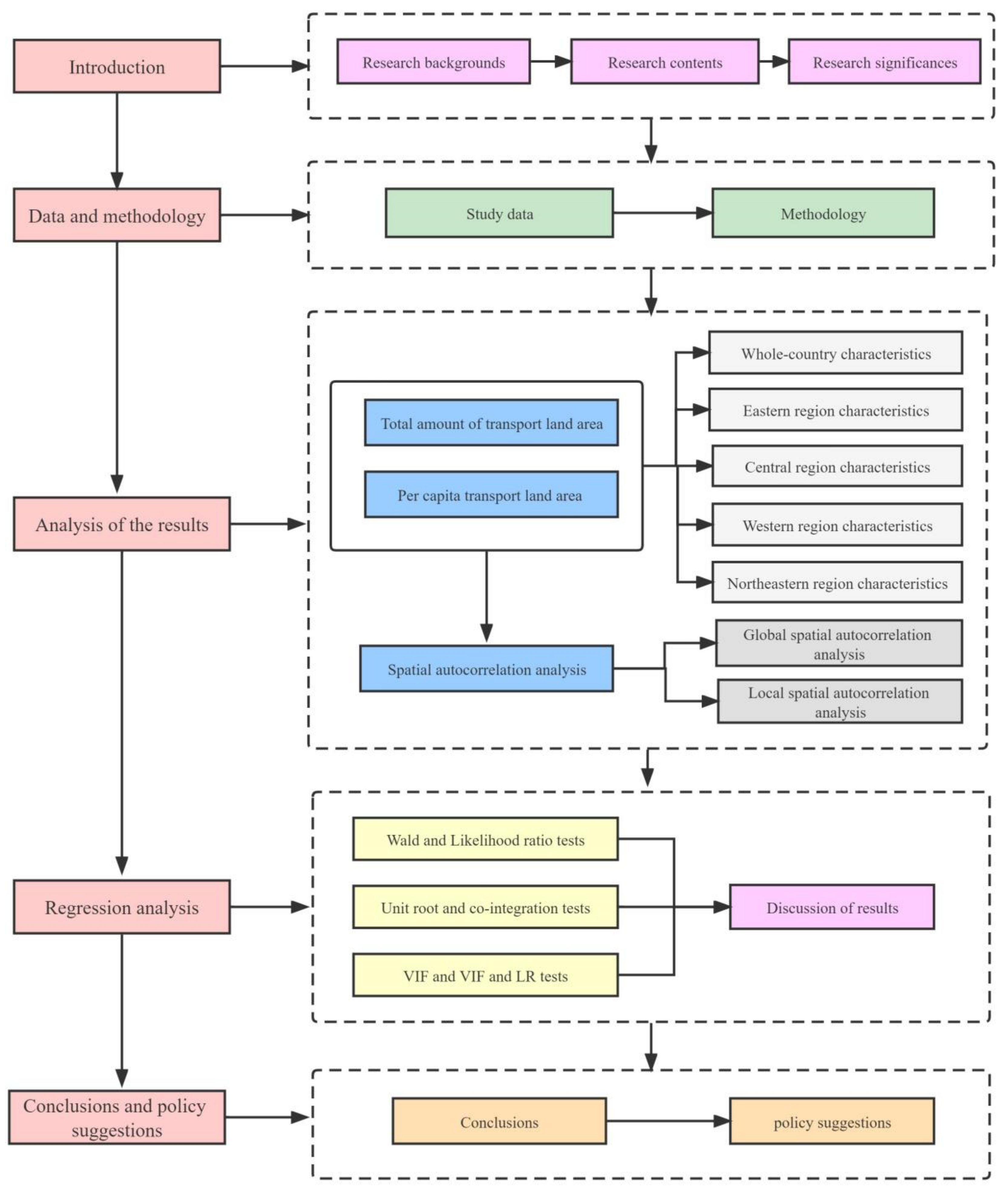
:1. Introduction
2. Data and Methodology
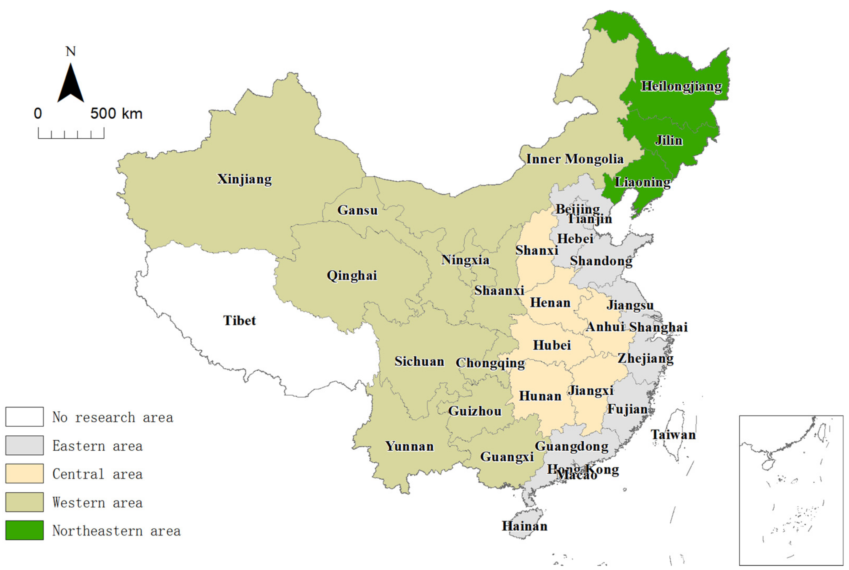
2.1. Data
2.2. Methodology
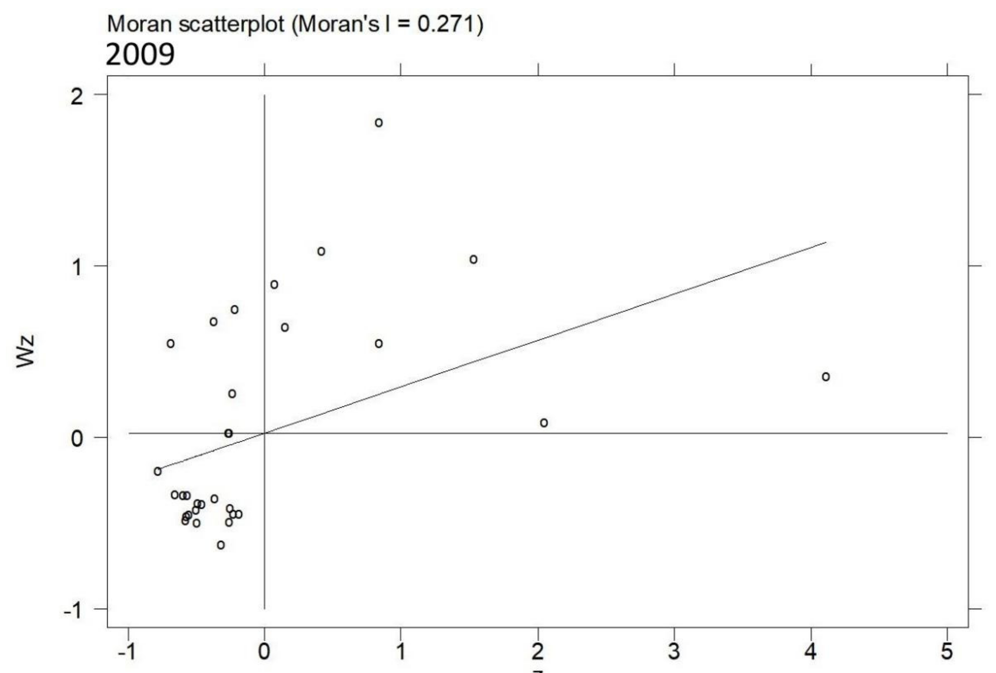
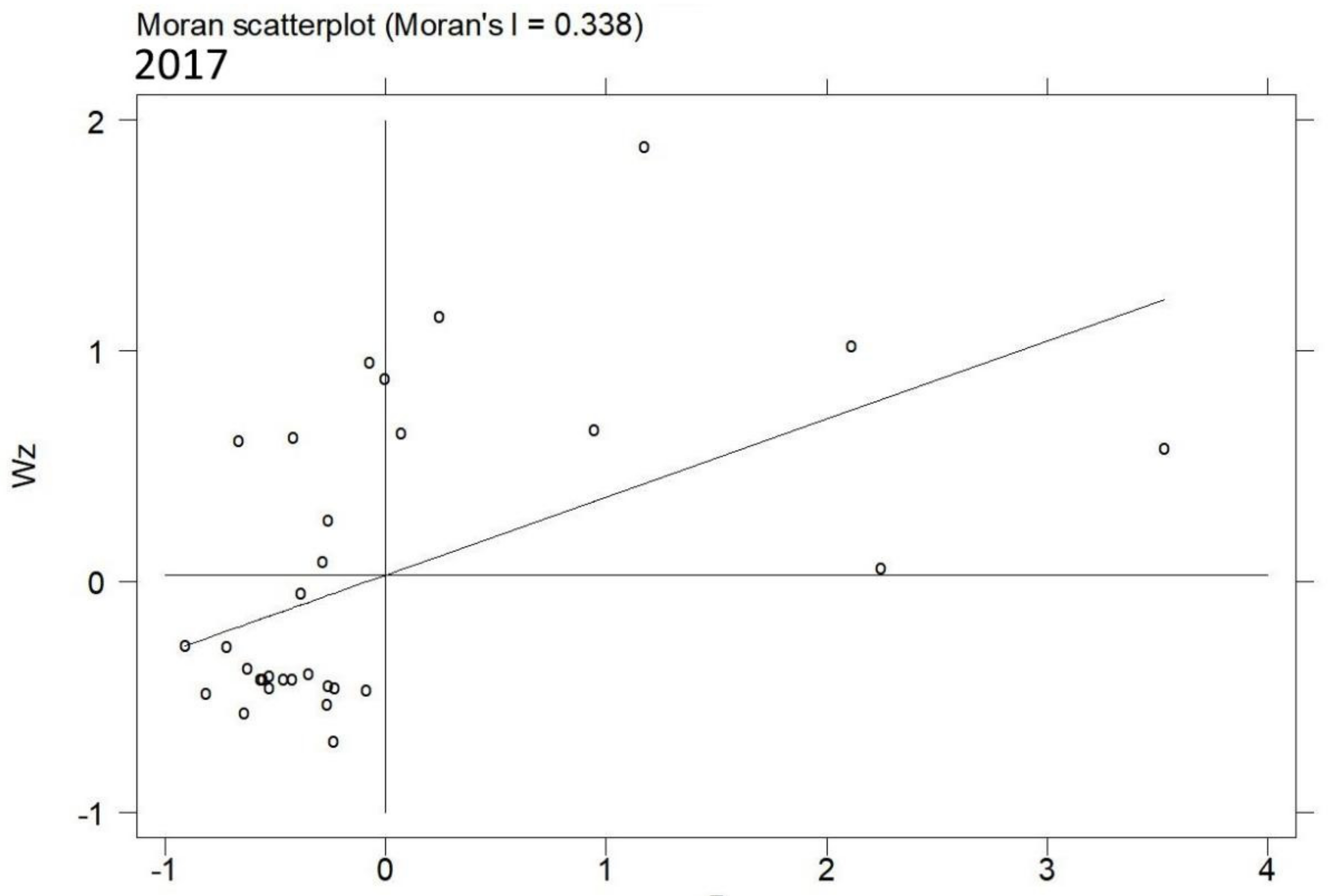
2.2.1. Spatial Autocorrelation Analysis
2.2.2. Spatial Durbin Model (SDM)
3. Analysis of the Results
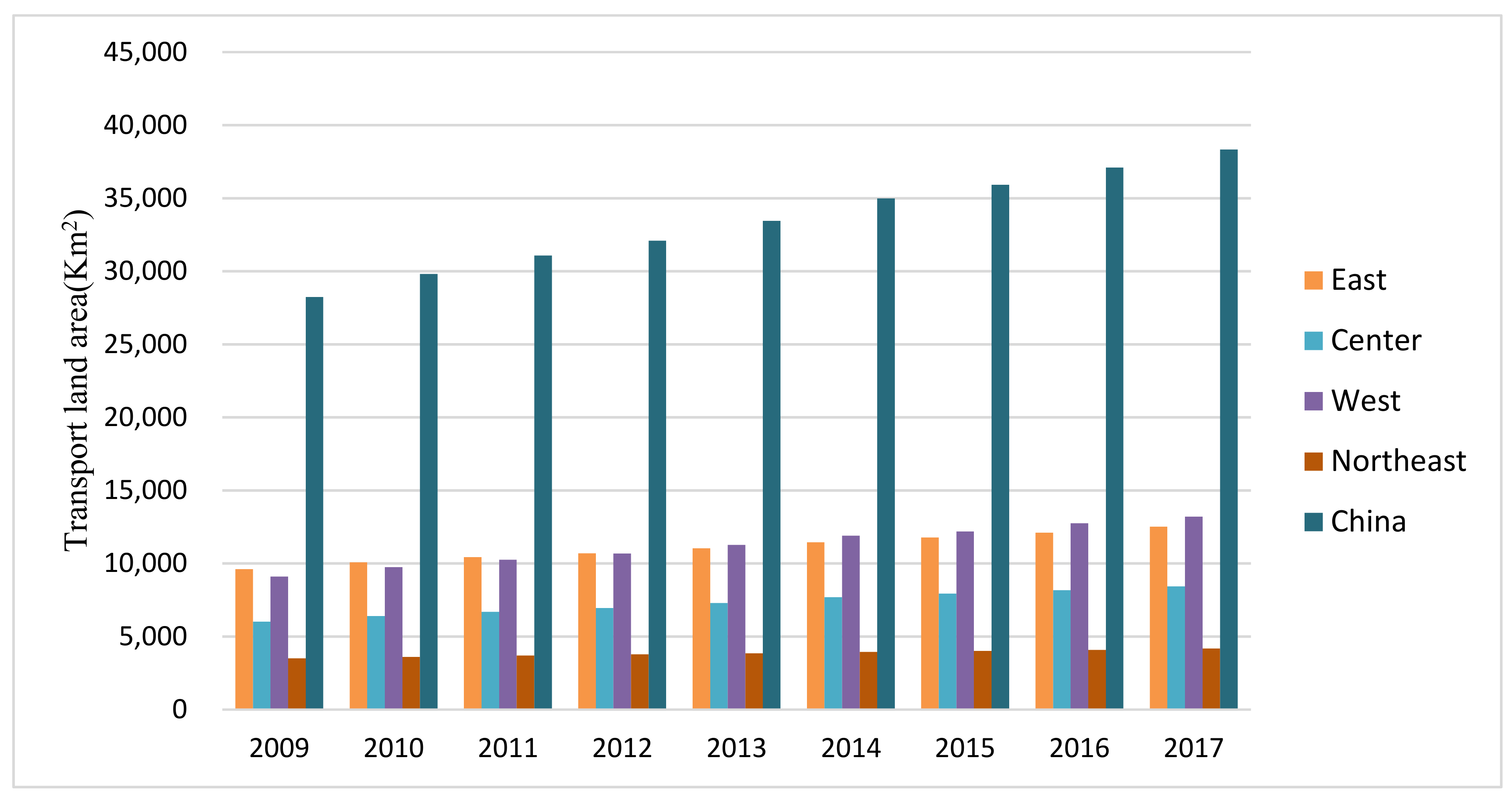
3.1. Total Amount of Transport Land Area
3.1.1. Whole-Country Characteristics
3.1.2. Eastern Region Characteristics
3.1.3. Central Region Characteristics
3.1.4. Western Region Characteristics
3.1.5. Northeastern Region Characteristics
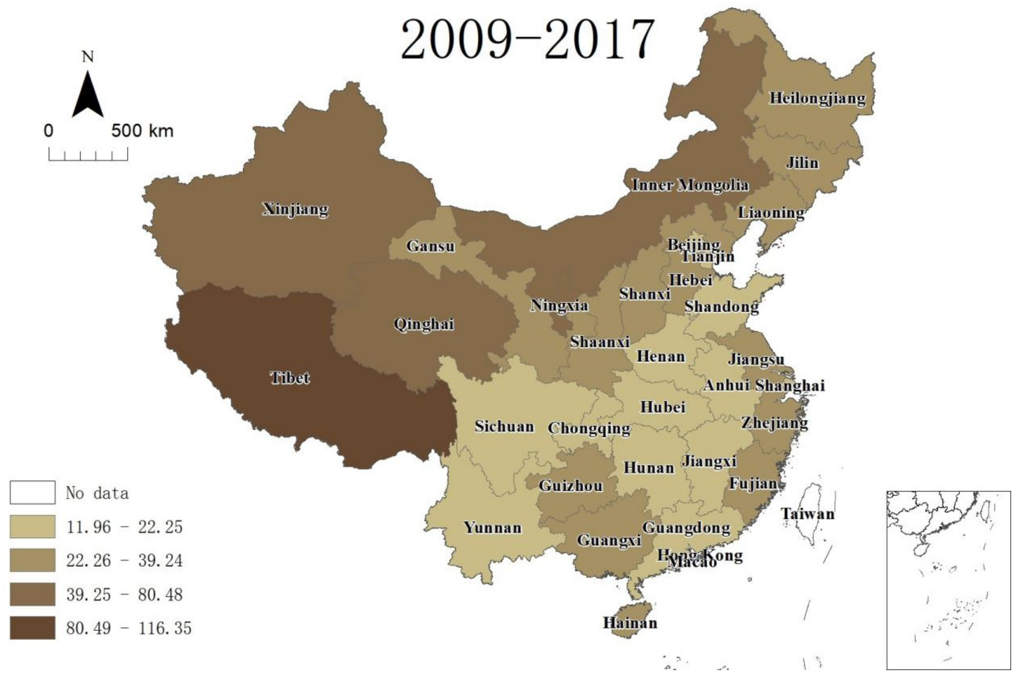
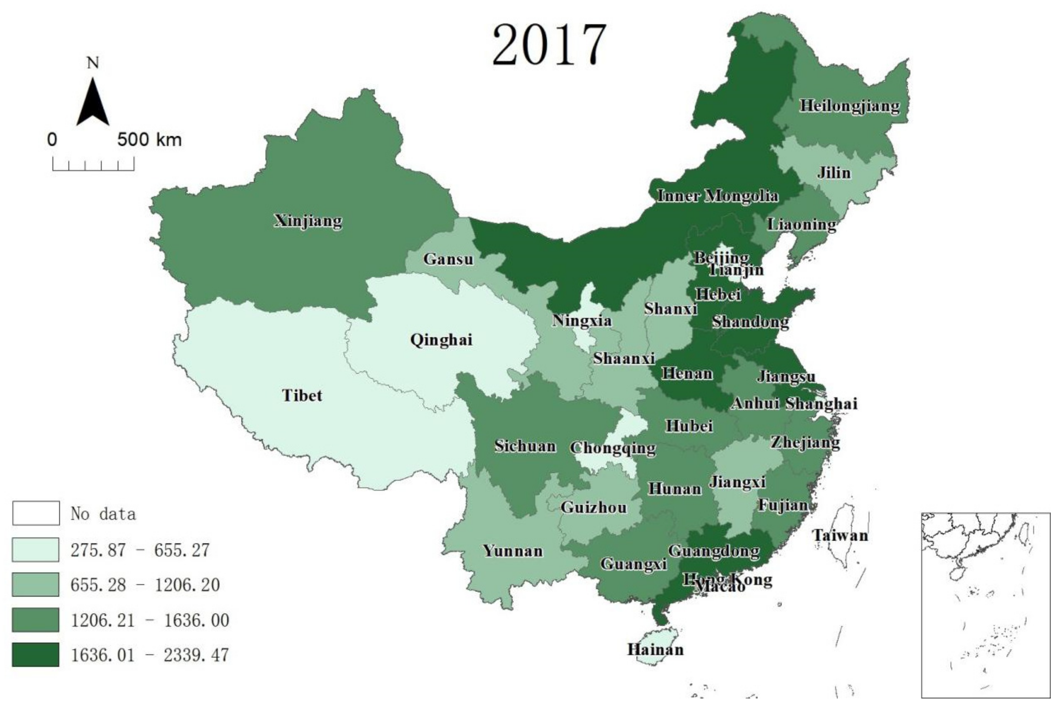
3.2. Per Capita Transport Land Area (PCTLA)
3.2.1. The Whole Country Characteristics
3.2.2. Eastern Region Characteristics
3.2.3. Central Region Characteristics
3.2.4. Western Region Characteristics
3.2.5. Northeastern Region Characteristics
3.3. Spatial Autocorrelation Analysis
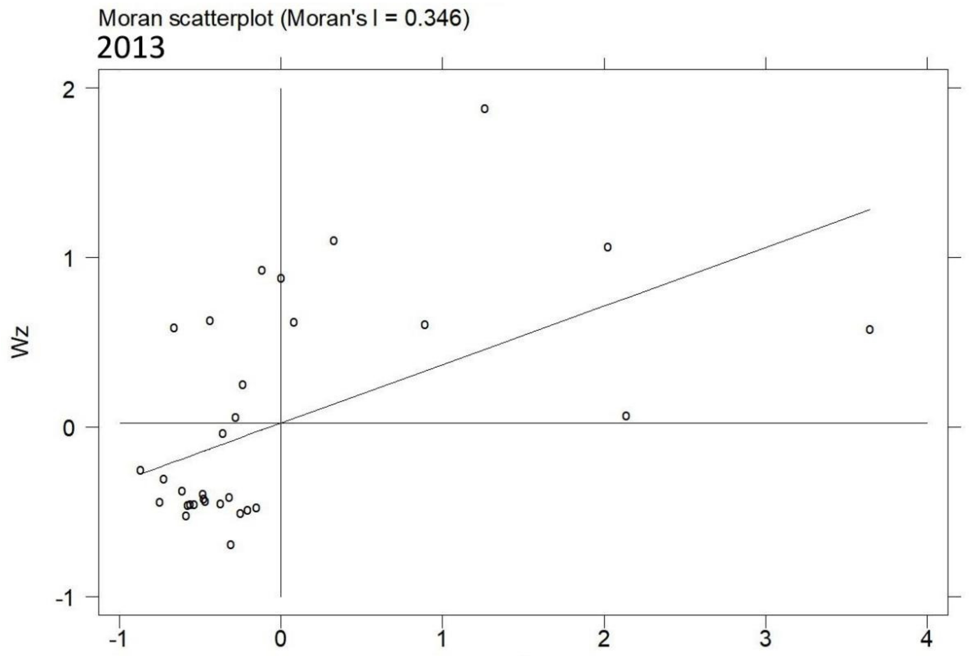
3.3.1. Global Spatial Autocorrelation Analysis
3.3.2. Local Spatial Autocorrelation Analysis
4. Regression Analysis
4.1. Wald and Likelihood Ratio Tests
4.2. Unit Root and Co-Integration Tests
4.3. VIF and LR Tests
β5 × ULi,t + β6 × TSi,t + θ1 × WDELi,t + θ2 × WGRi,t + θ3 × WISi,t + θ4 × WOULi,t +
θ5 × WULi,t + θ6 × WTSi,t + εi,t
εi,t ~ N(0,σ2i,t In),
4.4. Discussion of Results
5. Conclusions and Policy Suggestions
Author Contributions
Funding
Institutional Review Board Statement
Informed Consent Statement
Data Availability Statement
Conflicts of Interest
References
- Song, X.P.; Hansen, S.V.; Stehman, P.V.; Potapov, A.; Tyukavina, E.F.; Vermote, J.R. Townshend Global land change from 1982 to 2016. Nature 2018, 560, 639–643. [Google Scholar] [CrossRef] [PubMed]
- Zhou, B.B.; Aggarwal, R.; Wu, J.; Lv, L. Urbanization-associated farmland loss: A macro-micro comparative study in China. Land Use Policy 2020, 101, 105228. [Google Scholar] [CrossRef]
- Liu, J.Y.; Deng, X.Z.; Liu, M.L.; Zhang, S.W. Study on the spatial patterns of land-use change and analyses of driving forces in Northeastern China during 1990–2000. Chin. Geograph. Sci. 2002, 12, 299–308. [Google Scholar] [CrossRef]
- Liu, J.; Liu, M.; Zhuang, D.; Zhang, A.; Deng, X. Study on spatial pattern of land-use change in China during 1995–2000. Sci. China Ser. D-Earth Sci. 2003, 46, 373–384. [Google Scholar] [CrossRef]
- Gao, Z.; Liu, J.; Deng, X. Spatial features of land use/land cover change in the United States. J. Geogr. Sci. 2003, 13, 63–70. [Google Scholar] [CrossRef]
- Guo, L.; Wang, D.; Qiu, J.; Wang, L.; Liu, Y. Spatio-temporal patterns of land use change along the Bohai Rim in China during 1985–2005. J. Geogr. Sci. 2009, 19, 568–576. [Google Scholar] [CrossRef]
- Liu, J.; Zhang, Z.; Xu, X.; Kuang, W.; Zhou, W.; Zhang, S.; Li, R.; Yan, C.; Yu, D.; Wu, S.; et al. Spatial patterns and driving forces of land use change in China during the early 21st century. J. Geogr. Sci. 2010, 20, 483–494. [Google Scholar] [CrossRef]
- Ning, J.; Liu, J.; Kuang, W.; Xu, X.; Zhang, S.; Yan, C.; Li, R.; Wu, S.; Hu, Y.; Du, G.; et al. Spatiotemporal patterns and characteristics of land-use change in China during 2010–2015. J. Geogr. Sci. 2018, 28, 547–562. [Google Scholar] [CrossRef] [Green Version]
- Li, Z.; Song, G.; Lü, H.; Bao, Y.; Gao, J.; Wang, H.; Xu, T.; Cheng, Y. Analysis of land use change and its driving force in the Longitudinal Range-Gorge Region. Chin. Sci. Bull. 2007, 52, 10–20. [Google Scholar] [CrossRef]
- Jiang, Y.; Liu, J.; Cui, Q.; An, X.; Wu, C. Land use/land cover change and driving force analysis in Xishuangbanna Region in 1986–2008. Front. Earth Sci. 2011, 5, 288–293. [Google Scholar] [CrossRef]
- Liu, Y.; Wu, K.; Cao, H. Land-use change and its driving factors in Henan province from 1995 to 2015. Arab. J. Geosci. 2022, 15, 247. [Google Scholar] [CrossRef]
- Zhang, H.; Uwasu, M.; Hara, K.; Yabar, H. Sustainable Urban Development and Land Use Change—A Case Study of the Yangtze River Delta in China. Sustainability 2011, 3, 1074–1089. [Google Scholar] [CrossRef] [Green Version]
- Gao, J.; Wei, Y.D.; Chen, W.; Yenneti, K. Urban Land Expansion and Structural Change in the Yangtze River Delta, China. Sustainability 2015, 7, 10281–10307. [Google Scholar] [CrossRef] [Green Version]
- Chen, J.; Gao, J.; Yuan, F.; Wei, Y.D. Spatial Determinants of Urban Land Expansion in Globalizing Nanjing, China. Sustainability 2016, 8, 868. [Google Scholar] [CrossRef] [Green Version]
- Li, C.; Wu, K.; Wu, J. Urban land use change and its socio-economic driving forces in China: A case study in Beijing, Tianjin and Hebei region. Environ. Dev. Sustain. 2018, 20, 1405–1419. [Google Scholar] [CrossRef]
- Qian, J.; Zhou, Q.; Chen, X.; Sun, B. A Model-Based Analysis of Spatio-Temporal Changes of the Urban Expansion in Arid Area of Western China: A Case Study in North Xinjiang Economic Zone. Atmosphere 2020, 11, 989. [Google Scholar] [CrossRef]
- Kuang, W.H.; Liu, J.Y.; Dong, J.W.; Chi, W.F.; Zhang, C. The rapid and massive urban and industrial land expansions in China between 1990 and 2010: A CLUD based analysis of their trajectories, patterns, and drivers. Landsc. Urban Plan. 2016, 145, 21–33. [Google Scholar] [CrossRef]
- Kang, L.; Ma, L. Expansion of Industrial Parks in the Beijing–Tianjin–Hebei Urban Agglomeration: A Spatial Analysis. Land 2021, 10, 1118. [Google Scholar] [CrossRef]
- Park, J.; Kim, J.O. Does industrial land sprawl matter in land productivity? A case study of industrial parks of South Korea. J. Clean. Prod. 2022, 334, 130209. [Google Scholar] [CrossRef]
- Shi, Y.; Shi, Y. Spatio-Temporal Variation Characteristics and Driving Forces of Farmland Shrinkage in Four Metropolises in East Asia. Sustainability 2020, 12, 754. [Google Scholar] [CrossRef] [Green Version]
- Wang, J.; Wang, S.; Zhou, C. Quantifying embodied cultivated land-use change and its socioeconomic driving forces in China. Appl. Geogr. 2021, 137, 102601. [Google Scholar] [CrossRef]
- Zhang, J.; Yan, J.; Xue, L.; Yao, Y.; Shu, X. Is there a regularity: The change of arable land use pattern under the influence of human activities in the Loess Plateau of China? Environ. Dev. Sustain. 2021, 23, 7156–7175. [Google Scholar] [CrossRef]
- Xiang, H.; Ma, Y.; Zhang, R.; Chen, H.; Yang, Q. Spatio-Temporal Evolution and Future Simulation of Agricultural Land Use in Xiangxi, Central China. Land 2022, 11, 587. [Google Scholar] [CrossRef]
- Gao, J.; Liu, X.; Wang, C.; Wang, Y.; Fu, Z.; Hou, P.; Lyu, N. Evaluating changes in ecological land and effect of protecting important ecological spaces in China. J. Geogr. Sci. 2021, 31, 1245–1260. [Google Scholar] [CrossRef]
- Yao, G.; Li, H.; Wang, N.; Zhao, L.; Du, H.; Zhang, L.; Yan, S. Spatiotemporal Variations and Driving Factors of Ecological Land during Urbanization—A Case Study in the Yangtze River’s Lower Reaches. Sustainability 2022, 14, 4256. [Google Scholar] [CrossRef]
- Wang, S.; Tao, Z.; Sun, P.; Chen, S.; Sun, H.; Li, N. Spatiotemporal variation of forest land and its driving factors in the agropastoral ecotone of northern China. J. Arid Land 2022, 14, 1–13. [Google Scholar] [CrossRef]
- Li, B.; Cao, X.; Xu, J.; Wang, W.; Ouyang, S.; Liu, D. Spatial–Temporal Pattern and Influence Factors of Land Used for transport at the County Level since the Implementation of the Reform and Opening-Up Policy in China. Land 2021, 10, 833. [Google Scholar] [CrossRef]
- Zhao, P.; Lyu, D.; Hu, H.; Cao, Y.; Xie, J.; Pang, L.; Zeng, L.; Zhang, T.; Yuan, D. Population-development oriented comprehensive modern transport system in China. Dili Xuebao/Acta Geogr. Sin. 2020, 75, 2699–2715. Available online: https://www.scopus.com/inward/record.uri?eid=2-s2.0-85098962061&doi=10.11821%2fdlxb202012011&partnerID=40&md5=270e79cdb27ca6f57cde65fc25170846 (accessed on 13 June 2022).
- China Land and Resources Statistical Yearbook (CLRSY). China Statistical Publishing House, Beijing. 2015–2018. Available online: https://data.cnki.net/yearbook/Single/N2021050066 (accessed on 13 June 2022).
- Tobler, W.R. A computer movie simulating urban growth in the Detroit region. Econ. Geogr. 1970, 46, 234–240. [Google Scholar] [CrossRef]
- Elhorst, J.P. Spatial Panel Data Models. In Spatial Econometrics. SpringerBriefs in Regional Science; Springer: Berlin/Heidelberg, Germany, 2014; Available online: https://ideas.repec.org/h/spr/sbrchp/978-3-642-40340-8_3.html (accessed on 13 June 2022).
- Liu, F.Y.; Liu, C.Z. Regional disparity, spatial spillover effects of urbanisation and carbon emissions in China. J. Clean. Prod. 2019, 241, 118226. [Google Scholar] [CrossRef]
- The China Statistical Yearbooks (CSY) (2009–2018). China Statistical Publishing House, Beijing, China, 2009–2018. Available online: http://tongji.oversea.cnki.net/oversea/engnavi/HomePage.aspx?id=N2017100312&name=YINFN&floor=1 (accessed on 13 June 2022).
- National Bureau of Statistics of China (NBSC), 2022. Available online: https://data.stats.gov.cn/easyquery.htm?cn=C01 (accessed on 13 June 2022).
- Lu, H.Y.; Zhao, P.J.; Zeng, L.E.; Hu, H.Y.; Wu, K.S.; Lv, D. Transport infrastructure and urban-rural income disparity: A municipal-level analysis in China. J. Transp. Geogr. 2022, 99, 103292. [Google Scholar] [CrossRef]
- Zeng, K.; Eastin, J. Do Developing Countries Invest Up? The Environmental Effects of Foreign Direct Investment from Less-Developed Countries. World Dev. 2012, 40, 2221–2233. [Google Scholar] [CrossRef]
- Ali, N.; Phoungthong, K.; Techato, K.; Ali, W.; Abbas, S.; Dhanraj, J.A.; Khan, A. FDI, Green Innovation and Environmental Quality Nexus: New Insights from BRICS Economies. Sustainability 2022, 14, 2181. [Google Scholar] [CrossRef]
- Chen, F.; Zhao, T.; Liao, Z. The impact of technology-environmental innovation on CO2 emissions in China’s transportation sector. Environ. Sci. Pollut. Res. 2020, 27, 29485–29501. [Google Scholar] [CrossRef]
- Du, Q.; Li, J.; Li, Y.; Huang, N.; Zhou, J.; Li, Z. Carbon inequality in the transportation industry: Empirical evidence from China. Environ. Sci. Pollut. Res. 2020, 27, 6300–6311. [Google Scholar] [CrossRef]
- Zhao, P.; Zeng, L.; Li, P.; Lu, H.; Hu, H.; Li, C.; Zheng, M.; Li, H.; Yu, Z.; Yuan, D.; et al. China’s transportation sector carbon dioxide emissions efficiency and its influencing factors based on the EBM DEA model with undesirable outputs and spatial Durbin model. Energy 2022, 238, 121934. [Google Scholar] [CrossRef]
- Zhao, P.J.; Zeng, L.E.; Lu, H.Y.; Zhou, Y.; Hu, H.Y.; Wei, X.Y. Green economic efficiency and its influencing factors in China from 2008 to 2017: Based on the super-SBM model with undesirable outputs and spatial Dubin model. Sci. Total Environ. 2020, 741, 140026. [Google Scholar] [CrossRef] [PubMed]
- Li, C.; Shi, H.; Zeng, L.; Dong, X. How Strategic Interaction of Innovation Policies between China’s Regional Governments Affects Wind Energy Innovation. Sustainability 2022, 14, 2543. [Google Scholar] [CrossRef]
- Mingran, W. Measurement and spatial statistical analysis of green science and technology innovation efficiency among Chinese Provinces. Environ. Ecol. Stat. 2021, 28, 423–444. [Google Scholar] [CrossRef]
- Guan, W.; Xu, S. Study of spatial patterns and spatial effects of energy eco-efficiency in China. J. Geogr. Sci. 2016, 26, 1362–1376. [Google Scholar] [CrossRef]
- Zeng, L. China’s Eco-Efficiency: Regional Differences and Influencing Factors Based on a Spatial Panel Data Approach. Sustainability 2021, 13, 3143. [Google Scholar] [CrossRef]
- Li, C.Y.; Zhang, Y.Z.; Zhang, S.Q.; Wang, J.M. Applying the Super-EBM model and spatial Durbin model to examining total-factor ecological efficiency from a multi-dimensional perspective: Evidence from China. Environ. Sci. Pollut. Res. 2022, 29, 2183–2202. [Google Scholar] [CrossRef]
- Elhorst, J.P. Applied spatial econometrics: Raising the bar. Spat. Econ. Anal. 2010, 5, 9–28. [Google Scholar] [CrossRef]
- Long, R.Y.; Shao, T.X.; Chen, H. Spatial econometric analysis of China’s province-level industrial carbon productivity and its influencing factors. Appl. Energy 2016, 166, 210–219. [Google Scholar] [CrossRef]
- Zhao, L.S.; Sun, C.Z.; Liu, F.C. Interprovincial two-stage PCTLA under environmental constraint and spatial spillover effects in China. J. Clean. Prod. 2017, 164, 715–725. [Google Scholar] [CrossRef]
- Chen, Y.; Zhu, B.; Sun, X.; Xu, G. Industrial environmental efficiency and its influencing factors in China: Analysis based on the Super-SBM model and spatial panel data. Environ. Sci. Pollut. Res. 2020, 27, 44267–44278. [Google Scholar] [CrossRef]
- Qin, X.; Du, D.; Kwan, M.P. Spatial spillovers and value chain spillovers: Evaluating regional R&D efficiency and its spillover effects in China. Scientometrics 2019, 119, 721–747. [Google Scholar] [CrossRef]
- Li, T.; Han, Y.; Li, Y.; Lu, Z.; Zhao, P. Urgency, development stage and coordination degree analysis to support differentiation management of water pollution emission control and economic development in the eastern coastal area of China. Ecol. Indic. 2016, 71, 406–415. [Google Scholar] [CrossRef]
- Ning, L.; Zheng, W.; Zeng, L. Research on China’s Carbon Dioxide Emissions Efficiency from 2007 to 2016: Based on Two Stage Super Efficiency SBM Model and Tobit Model. Beijing Daxue Xuebao (Ziran Kexue Ban)/Acta Sci. Nat. Univ. Pekin. 2021, 57, 181–188. Available online: https://www.scopus.com/inward/record.uri?eid=2-s2.0-85101373648&doi=10.13209%2fj.0479-8023.2020.111&partnerID=40&md5=d948ef3627771ac2ca544cbf07fbc229 (accessed on 13 June 2022).
- Zeng, L.; Lu, H.; Liu, Y.; Zhou, Y.; Hu, H. Analysis of Regional Differences and Influencing Factors on China’s Carbon Emission Efficiency in 2005–2015. Energies 2019, 12, 3081. [Google Scholar] [CrossRef] [Green Version]
- Hong, J.; Chu, Z.; Wang, Q. Transport infrastructure and regional economic growth: Evidence from China. Transport 2011, 38, 737–752. [Google Scholar] [CrossRef]
- Pradhan, R.P.; Arvin, M.B.; Nair, M. Urbanization, transportation infrastructure, ICT, and economic growth: A temporal causal analysis. Cities 2021, 115, 103213. [Google Scholar] [CrossRef]
- Li, C.; Lin, T.; Zhang, Z.; Xu, D.; Huang, L.; Bai, W. Can transport infrastructure reduce haze pollution in China? Environ. Sci. Pollut. Res. 2022, 29, 15564–15581. [Google Scholar] [CrossRef] [PubMed]


| Explanatory Variable | Definition and of the Variables | Pre-Judgment |
|---|---|---|
| Economic development level (EDL) | GDP per capita (104 RMB) | Unknown |
| Government regulation (IS) | Proportion of financial expenditures to GDP (%) | Positive |
| Industrial structure (IS) | Proportion of the added value of tertiary industry to GDP (%) | Positive |
| Transport structure (TS) | Proportion of railway freight volume to total freight volume (%) | Negative |
| Opening up level (OUL) | Proportion of foreign trade to GDP (%) | Unknown |
| Urbanization level (UL) | Proportion of the urban resident population to the total population (%) | Positive |
| Regions | Provinces | 2009 | 2010 | 2011 | 2012 | 2013 | 2014 | 2015 | 2016 | 2017 | Mean |
|---|---|---|---|---|---|---|---|---|---|---|---|
| East | Beijing | 15.7 | 15.4 | 15.0 | 15.1 | 14.9 | 14.9 | 14.8 | 15.0 | 15.1 | 15.1 |
| Tianjin | 17.9 | 18.3 | 18.6 | 18.3 | 18.6 | 18.7 | 19.1 | 19.2 | 19.5 | 18.7 | |
| Hebei | 21.9 | 22.5 | 22.8 | 23.2 | 23.7 | 24.7 | 25.3 | 25.7 | 25.9 | 24.0 | |
| Shanghai | 11.3 | 11.2 | 11.5 | 11.5 | 12.2 | 12.2 | 12.4 | 12.5 | 12.7 | 12.0 | |
| Jiangsu | 23.6 | 24.5 | 25.0 | 25.5 | 26.1 | 26.9 | 27.5 | 28.1 | 29.0 | 26.2 | |
| Zhejiang | 22.2 | 22.6 | 23.4 | 23.9 | 24.6 | 25.4 | 25.9 | 26.5 | 26.8 | 24.6 | |
| Fujian | 22.7 | 24.8 | 26.3 | 27.3 | 28.4 | 29.9 | 31.2 | 32.2 | 33.5 | 28.5 | |
| Shandong | 19.8 | 20.1 | 20.4 | 20.7 | 20.9 | 21.3 | 21.5 | 21.7 | 22.4 | 21.0 | |
| Guangdong | 13.9 | 14.2 | 14.8 | 15.0 | 15.5 | 16.2 | 16.5 | 17.0 | 17.5 | 15.6 | |
| Hainan | 20.9 | 22.3 | 23.1 | 23.8 | 24.8 | 26.0 | 27.2 | 27.8 | 29.8 | 25.1 | |
| Mean | 19.0 | 19.6 | 20.1 | 20.4 | 21.0 | 21.6 | 22.1 | 22.6 | 23.2 | 21.1 | |
| Central | Shanxi | 22.6 | 22.8 | 23.3 | 24.7 | 26.5 | 27.9 | 28.3 | 28.8 | 29.2 | 26.0 |
| Anhui | 17.3 | 18.7 | 19.6 | 20.5 | 21.0 | 22.0 | 22.4 | 23.2 | 23.9 | 21.0 | |
| Jiangxi | 17.0 | 18.6 | 19.9 | 20.5 | 21.2 | 22.6 | 23.9 | 24.5 | 25.0 | 21.5 | |
| Henan | 15.1 | 15.9 | 16.7 | 17.1 | 18.0 | 18.8 | 19.1 | 19.0 | 19.8 | 17.7 | |
| Hubei | 15.6 | 16.5 | 16.8 | 17.6 | 18.8 | 20.1 | 20.7 | 21.7 | 22.3 | 18.9 | |
| Hunan | 17.2 | 18.2 | 19.0 | 19.2 | 19.7 | 20.3 | 20.7 | 21.2 | 21.6 | 19.7 | |
| Mean | 17.5 | 18.5 | 19.2 | 19.9 | 20.9 | 21.9 | 22.5 | 23.1 | 23.7 | 20.8 | |
| West | Inner Mongolia | 69.9 | 73.1 | 74.4 | 75.7 | 79.9 | 83.0 | 85.0 | 90.7 | 92.5 | 80.5 |
| Guangxi | 22.0 | 24.2 | 25.5 | 26.8 | 27.1 | 27.8 | 28.0 | 28.5 | 29.2 | 26.6 | |
| Chongqing | 15.4 | 16.6 | 17.4 | 18.2 | 19.1 | 19.8 | 20.3 | 20.8 | 21.3 | 18.8 | |
| Sichuan | 13.3 | 15.2 | 15.9 | 16.3 | 16.9 | 17.7 | 18.0 | 18.4 | 18.9 | 16.7 | |
| Guizhou | 15.9 | 18.0 | 20.2 | 21.6 | 23.4 | 26.3 | 26.9 | 28.4 | 29.9 | 23.4 | |
| Yunnan | 19.7 | 20.1 | 21.1 | 21.4 | 21.9 | 23.1 | 23.6 | 24.2 | 25.1 | 22.2 | |
| Tibet | 112.7 | 112.1 | 114.6 | 113.2 | 113.9 | 115.3 | 115.8 | 124.5 | 125.1 | 116.3 | |
| Shaanxi | 22.0 | 23.0 | 23.5 | 24.6 | 25.5 | 26.8 | 27.4 | 28.0 | 28.5 | 25.5 | |
| Gansu | 22.9 | 24.2 | 26.1 | 27.3 | 29.1 | 30.8 | 31.4 | 32.8 | 33.8 | 28.7 | |
| Qinghai | 59.3 | 63.8 | 67.0 | 68.3 | 77.4 | 83.4 | 83.6 | 88.1 | 89.2 | 75.6 | |
| Ningxia | 44.9 | 46.8 | 47.8 | 49.5 | 51.8 | 54.0 | 55.4 | 57.6 | 59.6 | 51.9 | |
| Xinjiang | 44.9 | 50.3 | 53.0 | 56.0 | 60.2 | 62.0 | 61.9 | 63.4 | 65.4 | 57.5 | |
| Mean | 38.6 | 40.6 | 42.2 | 43.2 | 45.5 | 47.5 | 48.1 | 50.4 | 51.5 | 45.3 | |
| Northeast | Liaoning | 30.5 | 31.1 | 31.9 | 33.0 | 33.6 | 34.3 | 35.2 | 35.8 | 37.4 | 33.7 |
| Jilin | 29.0 | 29.3 | 30.4 | 30.8 | 31.8 | 33.1 | 33.5 | 34.6 | 35.5 | 32.0 | |
| Heilongjiang | 36.1 | 37.3 | 38.2 | 38.8 | 39.2 | 39.8 | 40.7 | 41.4 | 41.8 | 39.2 | |
| Mean | 31.9 | 32.6 | 33.5 | 34.2 | 34.9 | 35.7 | 36.5 | 37.3 | 38.2 | 35.0 | |
| China | 21.2 | 22.2 | 23.0 | 23.6 | 24.5 | 25.4 | 26.0 | 26.6 | 27.4 | 24.4 | |
| Year | Moran’s I | Z-Score | p-Value |
|---|---|---|---|
| 2009 | 0.271 *** | 3.058 | 0.002 |
| 2010 | 0.296 *** | 3.209 | 0.001 |
| 2011 | 0.307 *** | 3.303 | 0.001 |
| 2012 | 0.322 *** | 3.392 | 0.001 |
| 2013 | 0.346 *** | 3.528 | 0.001 |
| 2014 | 0.352 *** | 3.549 | 0.000 |
| 2015 | 0.346 *** | 3.489 | 0.000 |
| 2016 | 0.334 *** | 3.405 | 0.001 |
| 2017 | 0.338 *** | 3.422 | 0.001 |
| Fixed Effects | Random Effects | |
|---|---|---|
| Wald test spatial lag | 70.96 *** | 58.97 *** |
| LR test spatial lag | 62.93 *** | 53.24 *** |
| Wald test spatial error | 64.25 *** | 58.35 *** |
| LR test spatial error | 62.06 *** | 63.52 *** |
| LLC | IPS | Fisher-ADF | PP-ADF | |
|---|---|---|---|---|
| PCTLA | −6.60768 *** | 1.83930 | 64.6650 | 124.415 *** |
| DEL | 7.04412 | 10.9454 | 35.6990 | 75.7464 |
| GR | −4.12454 *** | 0.64406 | 64.2165 | 75.4905 |
| IS | 0.33945 | 4.68552 | 23.7020 | 18.0197 |
| OUL | −3.38313 *** | −0.00699 | 63.9570 | 55.9228 |
| UL | 0.43679 | 3.09024 | 60.6950 | 128.335 *** |
| TS | −10.8097 *** | −2.46638 *** | 96.8195 *** | 124.508 *** |
| △PCTLA | −18.6607 *** | −7.64791 *** | 183.482 *** | 207.988 *** |
| △DEL | −1.67760 ** | −1.20650 | 109.696 *** | 138.485 *** |
| △GR | −11.2683 *** | −4.49974 *** | 132.641 *** | 179.111 *** |
| △IS | −8.07446 *** | −2.37604 * | 95.5379 ** | 163.830 *** |
| △OUL | −13.5558 *** | −6.10816 *** | 160.520 *** | 202.712 *** |
| △UL | −43.1966 *** | −15.2702 *** | 231.852 *** | 264.114 *** |
| △TS | −12.3195 *** | −3.62334 *** | 121.600 *** | 157.152 *** |
| △△PCTLA | −19.1019 *** | −7.11403 *** | 178.995 *** | 258.801 *** |
| △△DEL | −20.3399 *** | −7.36711 *** | 175.295 *** | 215.905 *** |
| △△GR | −20.3610 *** | −7.47487 *** | 190.048 *** | 300.100 *** |
| △△IS | −22.9412 *** | −5.83187 *** | 146.495 *** | 159.424 *** |
| △△OUL | −11.1121 *** | −3.23622 *** | 111.226 *** | 149.422 *** |
| △△UL | −41.3933 *** | −14.0336 *** | 251.204 *** | 300.619 *** |
| △△TS | −18.7076 *** | −7.19147 *** | 181.980 *** | 269.499 *** |
| DEL | GR | IS | OUL | UL | TS | Mean VIF | |
|---|---|---|---|---|---|---|---|
| VIF | 5.91 | 1.95 | 1.49 | 3.13 | 8.45 | 1.49 | 3.74 |
| 1/VIF | 0.169 | 0.514 | 0.669 | 0.319 | 0.118 | 0.669 |
| Spatial Fixed Effects | Time Fixed Effects | Spatial and Time Fixed Effects | |
|---|---|---|---|
| DEL | 6.162 *** | 2.579 *** | 2.563 *** |
| GR | 96.775 *** | 12.651 ** | 17.451 *** |
| IS | 79.956 *** | 10.895 ** | 9.853 ** |
| OUL | −18.485 *** | 8.675 *** | 7.993 *** |
| UL | −0.296 | 36.232 *** | 40.009 *** |
| TS | 32.632 *** | −44.135 *** | −46.854 *** |
| W*DEL | −12.447 *** | −4.058 *** | −4.041 *** |
| W*GR | 25.776 * | 46.310 *** | 63.479 *** |
| W*IS | 67.294 *** | −18.218 *** | −18.856 * |
| W*OUL | 37.527 *** | −11.969 *** | −13.642 |
| W*UL | 97.730 *** | 7.953 | 14.247 *** |
| W*TS | 21.284 | 29.439 *** | 17.175 |
| Spatial rho | 0.169 ** | 0.327 *** | 0.207 ** |
| Variance sigma2_e | 88.135 *** | 2.861 *** | 2.665 *** |
| R-squared | 0.199 *** | 0.731 | 0.729 |
| Log-likelihood | −1021.641 *** | −546.195 | −534.057 |
Publisher’s Note: MDPI stays neutral with regard to jurisdictional claims in published maps and institutional affiliations. |
© 2022 by the authors. Licensee MDPI, Basel, Switzerland. This article is an open access article distributed under the terms and conditions of the Creative Commons Attribution (CC BY) license (https://creativecommons.org/licenses/by/4.0/).
Share and Cite
Zeng, L.; Li, H.; Wang, X.; Yu, Z.; Hu, H.; Yuan, X.; Zhao, X.; Li, C.; Yuan, D.; Gao, Y.; et al. China’s Transport Land: Spatiotemporal Expansion Characteristics and Driving Mechanism. Land 2022, 11, 1147. https://doi.org/10.3390/land11081147
Zeng L, Li H, Wang X, Yu Z, Hu H, Yuan X, Zhao X, Li C, Yuan D, Gao Y, et al. China’s Transport Land: Spatiotemporal Expansion Characteristics and Driving Mechanism. Land. 2022; 11(8):1147. https://doi.org/10.3390/land11081147
Chicago/Turabian StyleZeng, Liangen, Haitao Li, Xiao Wang, Zhao Yu, Haoyu Hu, Xinyue Yuan, Xuhai Zhao, Chengming Li, Dandan Yuan, Yukun Gao, and et al. 2022. "China’s Transport Land: Spatiotemporal Expansion Characteristics and Driving Mechanism" Land 11, no. 8: 1147. https://doi.org/10.3390/land11081147
APA StyleZeng, L., Li, H., Wang, X., Yu, Z., Hu, H., Yuan, X., Zhao, X., Li, C., Yuan, D., Gao, Y., Nie, Y., & Huang, L. (2022). China’s Transport Land: Spatiotemporal Expansion Characteristics and Driving Mechanism. Land, 11(8), 1147. https://doi.org/10.3390/land11081147