Abstract
Healthy soils are fundamental for sustainable agriculture. Soil Improving Cropping Systems (SICS) aim to make land use and food production more sustainable. To evaluate the effect of SICS at EU scale, a modelling approach was taken. This study simulated the effects of SICS on two principal indicators of soil health (Soil Organic Carbon stocks) and land degradation (soil erosion) across Europe using the spatially explicit PESERA model. Four scenarios with varying levels and combinations of cover crops, mulching, soil compaction alleviation and minimum tillage were implemented and simulated until 2050. Results showed that while in the scenario without SICS, erosion slightly increased on average across Europe, it significantly decreased in the scenario with the highest level of SICS applied, especially in the cropping areas in the central European Loess Belt. Regarding SOC stocks, the simulations show a substantial decrease for the scenario without SICS and a slight overall decrease for the medium level scenario and the scenario with a mix of high, medium and no SICS. The scenario with a high level of SICS implementation showed an overall increase in SOC stocks across Europe. Potential future improvements include incorporating dynamic land use, climate change and an optimal spatial allocation of SICS.
1. Introduction
A well-functioning, healthy soil is fundamental for sustainable agriculture. Soil quality and soil health are increasingly considered important topics on the political and public agenda (e.g., [1,2]), and are also getting attention in the scientific community (e.g., [3,4]). This is reflected in, among others, the Sustainable Development Goals (SDGs; https://sdgs.un.org/goals (accessed on 12 April 2022)), where soil together with land use and management play an important role in SDG 1 (no poverty), 2 (zero hunger), 12 (responsible consumption and production), 13 (climate action) and especially SDG 15 (Life on Land) [2,5]. Moreover, in the current Farm to Fork Strategy (F2F, [6]), as part of the European Green Deal [7], sustainable food production is an important goal; the F2F aims at neutral or positive environmental impact, mitigating climate change, reversing the loss of biodiversity and ensuring food security. Land use and land management play a key role in achieving these policy aims and reversing the current trend of land degradation [8]. For example, the F2F strategy targets to ‘bring back at least 10% of agricultural areas under high-diversity landscape features (with buffer strips, rotational or non-rotational fallow land, hedges, non-productive trees, terrace walls and ponds)’ and ‘have 25% of the EU’s agricultural land as organic farming by 2030’ [9]. These strategies are also developed as the costs of unsustainable land management are estimated to exceed €50 billion per year [10].
The measures mentioned in the F2F strategy are only a few of the very many existing land management options to improve soil health and reverse or prevent land degradation, ranging from farm and field to village and watershed or community scales (e.g., [11,12] and https://qcat.wocat.net/en/wocat/ (accessed on 12 April 2022)). Among those many options, some measures are common in annual and perennial agriculture across Europe. For example, maintaining a (winter) cover crop is widely applied [13,14,15]. No-tillage or minimum tillage has been estimated to be applied on 25% of the agricultural land in the EU [16]. Mulching is applied to reduce splash erosion and increase soil moisture [17,18]. Crop residue management [19] and/or maintaining a minimum soil cover is also widely applied [12,17]. Grass strips are applied at field borders [20] to reduce runoff and catch sediments [18,21] and as a means to reduce leaching of nutrients [21,22] and/or pesticides [23]. Rodrigues et al. [19] for example show that reduced tillage and soil protective measures can play an important role in soil carbon sequestration across the EU. Maetens et al. [18] investigated the effect of various soil and water conservation measures on runoff and soil loss across Europe.
These practices affect the farming and cropping systems, aiming to make land use and food production more sustainable. As defined in Hessel et al. [24], cropping system refers to crop type, crop rotation and the agronomic management techniques used. Soil improving cropping systems (SICS) can be defined as cropping systems that result in a durable increased ability of the soil to fulfil its functions, including food and biomass production, buffering and filtering capacity and provision of other ecosystem services [24]. However, the uptake and choice of SICS will vary due to external factors, such as EU policies, market effects, society and pedo-climatic conditions. In addition, these factors are dynamic in time as they are affected by e.g., climate change, geo-politics, consumer purchase power and preferences, technological advances and other developments [25,26]. Hence, when assessing the effects of SICS on improving soil health and combatting land degradation at continental scale it is important to consider divergent trends in these factors that affect the uptake of SICS (e.g., [26,27]).
Soil health and land degradation are both broad terms [2] that include many aspects. Soil health has been defined as the continued capacity of soil to function as a vital living ecosystem that sustains plants, animals and humans [3]; encompasses biological productivity, soil life and biodiversity; enhances its role in water quality and regulation and mitigates climate change. Similarly, land degradation entails many different processes, such as salinisation, nutrient depletion, dehydration, erosion by water or wind, compaction, soil pollution, loss of soil organic matter and soil biodiversity etc., [28,29,30,31]. In this study, we focused on one principal indicator for each aspect: Soil Organic Carbon (SOC) as a principal indicator for soil health [32,33] and soil erosion (by water) as an indicator and widely occurring process of land degradation [34,35]. Moreover, Kutter et al. [12] in their review on policy measures for agricultural soil conservation in the EU, found that most measures focused on erosion by water, followed by decline in organic matter.
Upscaling the assessment of the impact of measures from e.g., field or farm level to country or wider (e.g., EU) scale is challenging as measuring at this scale is infeasible [34]. Modelling is a common approach and can also include simulation of scenarios of e.g., climate change effects and policy adoption [36,37]. At EU wide scale, soil erosion was estimated by Panagos et al. [34], based on the RUSLE approach. EU wide SOC estimates include e.g., [38,39,40]. The RUSLE-based erosion estimates by Panagos et al. [34] also include the effect of mitigation options such as conservation tillage, plant residues and winter crop cover [16] and contour farming, stone walls and grass margins [41]. Modelling estimates of climate change and land use change effects on SOC are abundant, e.g., [42,43,44,45], and various studies quantified the effects of agricultural practices on carbon sequestration [46,47,48]. Lugato et al. [49] included straw incorporation, reduced tillage, their combination, ley cropping systems and cover crops into their spatially explicit modelling scenarios.
The SoilCare project (https://www.soilcare-project.eu/ (accessed on 12 April 2022) [24]) aimed to identify and evaluate promising soil improving cropping systems and agronomic techniques that increase the profitability and sustainability of agriculture across Europe. In addition to field trials [50,51], the project used a modelling approach to upscale the effects of SICS to EU scale, in a spatially explicit way. To ensure that sufficient healthy food for expanding human populations can be grown within planetary boundaries [52], soil management should aim at improving the health and resilience of land and soil [8]. In this study we evaluated how soil improving cropping systems (SICS) impact land degradation (specifically erosion) and soil health (specifically SOC stocks) across Europe, through the application of the PESERA model. For this purpose, we improved and further developed the PESERA model both in terms of input data improvements and in parameterisation and calibration of SICS and a range of crops, in four climate zones. Moreover, to be able to assess the impacts of SICS, existing land management options have been adapted in the model. Four scenarios, developed within the SoilCare project, were simulated until 2050, with varying application of (combinations of) SICS in each scenario.
2. Methods
2.1. PESERA Model Description
The Pan-European Soil Erosion Risk Assessment (PESERA) model simulates biophysical processes including above-ground biomass production, soil erosion risk, soil water deficit and soil humus content, using a monthly time-step. The model was originally developed by Kirkby et al., [53] and has been applied in various agro-ecological zones e.g., [54,55,56,57]. A brief technical description is given here, based on Kirkby et al. [53], where all details can be found. PESERA is a process-based and spatially distributed model which combines the effect of topography, climate and soil properties. A schematic model structure is provided in Figure 1. The model has three conceptual stages: (i) A storage threshold model to convert daily rainfall to daily total overland flow runoff; (ii) a power law to estimate sediment transport from runoff and slope gradient. The model interprets sediment transported to the base of a hillslope as average erosion loss. No flow or sediment routing over multiple cells is included; and (iii) integration of daily rates over the frequency distribution of daily rainfalls to estimate monthly erosion rates.
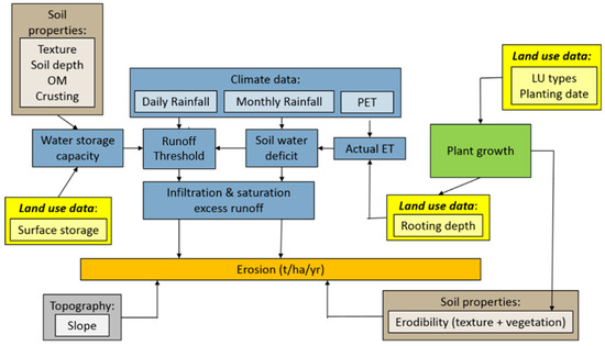
Figure 1.
Schematic overview of processes in the PESERA model.
In the first step, a simple storage or bucket model is used to convert daily rainfall into daily runoff, which is estimated as the rainfall minus the threshold storage. The threshold storage depends dynamically on soil properties, vegetation cover and soil moisture status, varying over the year. The most important soil factors that determine the threshold storage beneath the vegetation-covered fraction of the surface are texture, depth (if shallow) and organic matter. Where the surface is not protected by vegetation, the susceptibility of the soil to crusting and the duration of crusting conditions generally determine a lower threshold. The final threshold is a weighted average from vegetated and bare fractions of the surface. Corrections are made for the soil water deficit, which may reduce the threshold where the soil is close to saturation. Transpiration is used to drive a generic plant growth model for biomass, constrained as necessary by land use decisions, primarily on a monthly time step. Leaf fall also drives a simple model to estimate soil organic matter.
Precipitation is divided into daily storm events, expressed as a frequency distribution. The distribution of daily rainfall totals is fitted to a Gamma distribution for each month. The rainfall distribution, reflected by the coefficient of variation of rainfall per rain day is given for each month of the simulation period and may be adapted for (future) climate change scenarios. Daily precipitation drives infiltration, excess overland flow and soil erosion, and monthly precipitation, driving saturation levels in the soil. Infiltration excess overland flow is estimated from storm rainfall and soil moisture. Sediment transport is then estimated using a power law approach driven by erodibility, gradient and runoff discharge. Soil erodibility is derived from soil classification data, primarily texture (see Section 2.2.7). Local relief is defined as the standard deviation of elevation within a defined radius around each point (Section 2.2.1 and Figure 2). Accumulated runoff is derived from a biophysical model that combines the frequency of daily storm sizes with an assessment of runoff thresholds based on seasonal water deficit and vegetation growth. Estimates of sediment transport are based on infiltration excess overland flow discharge. In the PESERA model, sediment transport is interpreted as the mean sediment yield delivered to stream channels and includes no downstream routing within the channel network.
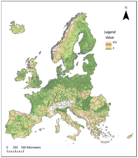
Figure 2.
Local relief (standard deviation of elevation in a 1500 m radius) for Europe.
The role of vegetation and soil organic matter can modify the infiltration rates through changes in soil structure and/or the development over time of surface or near-surface crusting. Three models are coupled to provide the dynamics of these responses: (i) A vertical hydrological balance, which partitions precipitation between evapotranspiration, overland flow, subsurface flow and changes in soil moisture; (ii) a vegetation growth model, which budgets living biomass and organic matter subject to the constraints of land use and cultivation choices; and (iii) a soil model, which estimates the required hydrological variables from moisture, vegetation and seasonal rainfall history.
The PESERA model works with two phases: an equilibrium phase and a simulation phase. The equilibrium phase model is run first: it calculates long-term average values, using long-term input data on e.g., climate. The equilibrium phase model is calibrated using long-term average data (see Section 2.3). Then, these long-term output maps are used to initiate the simulation phase model. This model uses monthly climate data to run future scenarios (see Section 2.4).
PESERA outputs consist of monthly maps of: vegetation biomass (ton/ha), erosion (risk) (ton/ha/y) and soil organic matter content (ton/ha) for each simulation year. Within the SoilCare project the following improvements were made in the PESERA model: additional crop types (sugar beets, rice, fodder versus consumption maize) have been parameterised and calibrated for Europe; all crops were parameterised and calibrated for four main climate zones across Europe and biomass and SOM were calibrated for each land use/crop type; irrigation has been added as an option in the model; erodibility information for the Northern countries (Norway, Sweden and Iceland) has been updated to solve issues with existing Europe-wide data (see Section 2.2) and soil management options (i.e., SICS) have been defined, parameterised and calibrated (see Section 2.3).
2.2. Input Data
The required model input data and their sources are summarised in Table 1. All input maps have a spatial resolution of 500 m and projection ETRS 1989 LAEA (Lambert Azimuthal Equal Area). The area modelled is the EU-28, i.e., the current 27 EU countries plus UK. Basic details and the most important maps are given here; a full description and all input maps are given in Supplementary Material S1.

Table 1.
Overview of PESERA input requirements.
2.2.1. Topography
One of the main variables in the model is local relief (Figure 2). It is estimated from the digital elevation model (DEM) as the standard deviation of elevation with a circle of 1.5 km (5 cell radius) diameter around each cell.
2.2.2. Climate
Climate input data differs slightly between the equilibrium and simulation phase models. For the equilibrium phase model, E-OBS version 21.0e data, at 0.1º spatial resolution and daily scale was used. Daily data for the ensemble mean of mean temperature, minimum temperature, maximum temperature and rainfall were collected for 1981–2010, representing the reference period used to bias-correct climate scenarios. The monthly parameters shown in Table 1 were calculated from these values, after being interpolated to a 500 m resolution. The data source is Cornes et al. [58]. Maps of the equilibrium climate input data are presented in Supplementary Material S1.
To minimise bias, climate scenarios at high resolution (0.1º), and already bias corrected with present-day climate (E-OBS) were used in the simulation phase model. The considered emission scenario was RCP4.5 (closer to the average of all emission scenarios). The selected GCM-RCM combination was MPI-ES-LR + CCLM4-8-17. This means that we used the MPI-ES-LR GCM, which has a median sensitivity to climate change [63] combined with the CCLM RCM, which appears to have less bias for temperature and rainfall in several European regions [64]. We used data from the JRC EU High Resolution and Precipitation dataset, which is already bias-corrected using E-OBS [60].
2.2.3. Land Use and Crop Data
The land use and crop map (Figure 3) was made within the SoilCare project, based on Corine Land Cover 2018 (CLC2018) (https://land.copernicus.eu/pan-european/corine-land-cover (accessed on 15 September 2021)) crop data from Eurostat (https://ec.europa.eu/eurostat (accessed on 15 September 2021)), and infrastructure (e.g., roads), zoning (e.g., protected natural areas, urban expansion plans) and crop suitability maps from Metronamica. Details on how these data were used to derive the SoilCare land use and crop map are given in [65].
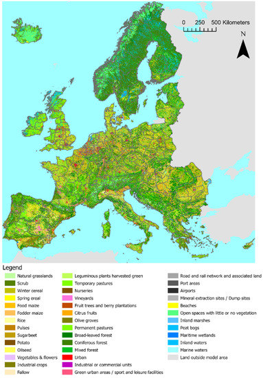
Figure 3.
SoilCare land use and crop map (year: 2018). A GIS compatible version of this map is available in the Supplementary Materials.
2.2.4. Crop Calendars: Planting Month, WUE and Cover
As crop calendars for the same crop may differ per climate region, we created four major agro-climatic regions in Europe, for which crop calendars were constructed for each crop. We did not use existing maps for cropping calendars, as they are either too coarse [66], not crop-specific [67], or represent related variables which are difficult to translate into planting month [68,69]. We decided instead to aggregate areas per climate region. The existing Köppen-Geiger system determines 19 different climate types in Europe [70]. These were aggregated into the six most representative classes, each occupying at least 5% of the SoilCare study area, and together occupying 92% of the total area; the remainder were assigned to the closest climate class. It should be noted that the division between climate regions is not sharp, and there are often climatic gradients. The six classes were then transformed into four classes with two further aggregations: (1) For cropping purposes, the dry climate regions are similar to the Mediterranean climate regions, so they were reclassified as the latter; and (2) polar climate is important in a large part of mountain regions, but agriculture is not practiced there, so for the model they were reclassified as subarctic climate. Figure 4 shows the climate zones as used in the modelling; they are similar to the environmental stratification of Europe proposed by Metzger et al. [71].
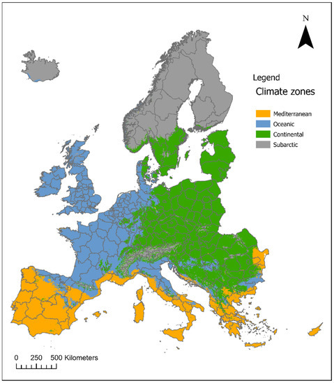
Figure 4.
Climate zones as used in SoilCare to vary crop calendars by agroclimatic zone.
Finally, we aggregated existing crop calendar information for different countries in Europe for the four climate zones using the following datasets according to the dominant climate in the country, in decreasing order of preference:
- (a)
- JRC crop calendars for winter wheat, grain maize and rice: https://agri4cast.jrc.ec.europa.eu/DataPortal/Index.aspx?o=sd (accessed on 15 December 2021)
- (b)
- USDA crop calendars for Europe: https://ipad.fas.usda.gov/rssiws/al/crop_calendar/europe.aspx (accessed on 15 December 2021) and https://ipad.fas.usda.gov/countrysummary/Default.aspx?id=E4 (accessed on 15 December 2021)
- (c)
- Boons-Prins et al. [72] with crop calendars for many crops in Europe: https://edepot.wur.nl/308997 (accessed on 15 December 2021)
When extended (>1 month) planting and harvesting dates were given, the latest planting and earliest harvesting date were chosen. The aggregation of calendars gave consistent planting and harvest dates for each region, with the Mediterranean region showing differences from the three other regions, either in earlier planting dates or shorter growing seasons. Cropping calendars were discussed with local partners from the SoilCare project and adapted according to their experience.
Monthly ground cover (%) for each crop was derived mostly from the PESERA project manual, with some exceptions or additions:
- Sugarbeet: estimated and adapted from potato
- Oilseed: estimates based on pictures in Corlouer et al. [73] and comparison with winter wheat
- Rice: taken from FAO http://www.fao.org/docrep/S2022E/s2022e07.htm (accessed on 15 December 2021)
These cover calendars were then adjusted to the crop calendars. In most cases, the cover calendars fit inside the planting and harvest dates. When they did not fit, they were adjusted to keep the same shape as the PESERA growth curves but fitting a shorter or longer interval as needed. When the crop calendars indicated planting or harvesting seasons longer than one month, the cover values of these seasons were extended by repeating the first or last month value (respectively). Table 2 shows the crop calendars per agroclimatic zone and crop, with the cover indicated as value. Monthly canopy cover for permanent crops were based on the PESERA project estimations [74] for Europe and are given in Table S1.
Table 2.
Crop calendar and ground cover values (%) per crop and agroclimatic zone. Dark green cells indicate the start of the growing season (planting month), orange cells indicate the last month of the growing season.
Water use efficiency values were calculated for different crops based on the following sources:
- For spring wheat, winter wheat, potato, sugarbeet, sunflower/tomato, bean (pulses): FAO http://www.fao.org/land-water/databases-and-software/crop-information/maize/en/ (accessed on 15 December 2021);
- For consumption maize (sweet maize) and fodder maize (grain maize): FAO http://www.fao.org/3/S2022E/s2022e07.htm (accessed on 15 December 2021);
- For oilseed (winter oilseed rape):
- Length of the growing stages: (Marjanović-Jeromela et al., 2019)
- Kc values: (Corlouer et al., 2019) (Figure 2 in their suppl. Material) [73]
- For rice: FAO paddy rice: http://www.fao.org/3/S2022E/s2022e07.htm (accessed on 15 December 2021)
- For forage: taken from PESERA manual [74].
WUE calendars, with crop- and growth stage specific WUE values, were also based on planting and harvest dates, and used the same method as that for cover calendars, including stretching or shortening curves to match planting and harvesting dates (Table S2).
2.2.5. Rooting Depth and Surface Storage
Rooting depth was estimated based on three sources: the PESERA project manual [74]; estimates from FAO: http://www.fao.org/land-water/databases-and-software/crop-information/maize/en/ (accessed on 15 October 2020). These estimates start at 30 cm root depth going to 100 cm at the end of the growing season. As PESERA estimates were lower, a conservative estimate was taken and cross-checked with the third source; the SWAT database, which also estimates slightly deeper (maximum) rooting depths. For initial surface storage (either 0, 5 or 10 mm) and reduction of surface storage (either 0 or 50%), the PESERA project manual was followed. Values of rooting depth, initial surface storage and reduction of surface storage used in this study are given in Table S3.
2.2.6. Soil Properties
Soil property data are used to calculate storage capacity and therefore the runoff threshold and affect plant growth through soil water availability. Six layers of soil data are required: (1) Erodibility, which is the sensitivity of the soil for erosion; (2) crusting, which is the sensitivity of the soil to surface crusting and affects the infiltration; (3) scale depth, which is a proxy for infiltration; (4) the effective soil water storage capacity; and soil water available to plants for depths 0–300 mm (5) and 300–1000 mm (6) respectively.
2.2.7. Erodibility
The erodibility map has five classes. We used the RUSLE erodibility K-factor, as prepared by Panagos et al., [61], with stoniness effects incorporated, grouped into five classes (Table S4). As indicated earlier (Section 2.3), based on discussions with local partners, the erodibility map for Norway, Sweden and Iceland was adapted. Details of the method used can be found in Supplementary Material S1. Figure 5 shows the final erodibility map as used in this study.
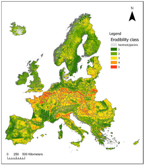
Figure 5.
Erodibility map as used in SoilCare. Note that bare rock and glacier areas (according to CLC2018) were excluded (grey colours).
2.2.8. Crusting and Scale Depth Maps
The soil sensitivity to crusting index map was created using pedotransfer functions on texture, parent material and physical–chemical soil properties (Figure S1). The scale depth input map (Figure S2) was derived from soil texture classes (Table S5). Texture data were derived from the ESDB database.
2.2.9. Soil Water Availability and Storage Maps
Soil water available to plants (both 0–30 and 30–100 cm) and effective soil water storage capacity maps were derived based on the instructions from the PESERA project [74] and using ESDB data. Available Water Content for topsoil and subsoil (AWC_top and AWC_sub) maps of ESDB were used as a starting point. Additional soil property data used in the pedotransfer functions include texture, packing density and restriction of soil depth by bedrock.
The effective soil water storage capacity was then calculated from the soil water available to plants in the top- and subsoil following the PESERA project instructions [74]. Estimations for Iceland and Cyprus, that are not included in the ESDB maps, were derived using the SWAT data in combination with the FAO Harmonized World Soil Database (HWSD), available at https://doi.pangaea.de/10.1594/PANGAEA.901309 (accessed on 15 August 2020). All three maps are shown in Supplementary Material S1 (Figures S3–S5).
2.3. Model Calibration and Evaluation
During the equilibrium phase, long-term average output of the model was calibrated for erosion estimates and soil organic matter. As it was not feasible to calibrate the model for all countries, calibration was carried out for four countries in various climate zones across Europe (Belgium Spain, Slovakia and Norway), and the Greek island of Crete. Tuning parameters for calibration were: (1) The biomass conversion factor used in the model to calculate gross primary production—affecting ground cover and thereby erosion; and (2) the decomposition factor used in the model to calculate soil organic matter from plant residues. Both parameters are specific for each crop and land use, but generic for all regions. For soil organic matter calibration, the LUCAS topsoil soil organic carbon point data was used: https://esdac.jrc.ec.europa.eu/projects/lucas (accessed on 1 December 2020), which was aggregated to crops and land covers per climate zone (Table S6). In addition, to cross-validate and make use of the knowledge of the SoilCare local partners, both the spatial patterns and numerical (aggregated) results were shared with selected countries across Europe and their feedback was used for further fine-tuning. Preliminary results were sent to partners in Belgium, Germany, Greece, Spain, Italy, Norway, Poland and Romania. Based on their feedback:
- The erodibility map for Norway was adapted because it had too high erodibility in the central mountain areas where soils are very shallow and granite bedrock is very often at the surface; hardly any erosion occurs in these areas. The existing K-factor map from JRC was adapted for certain land uses (following Corine Land Cover 2018), as detailed in Section 2.2
The model output at EU scale was evaluated by comparing the ranges and spatial patterns of the equilibrium phase PESERA erosion and SOC output maps to existing maps reported in the literature (for SOC e.g., [38,75,76,77]; for erosion e.g., [34,78,79]; see Supplementary Material S2.
2.4. Parameterisation of SICS
The PESERA model was used to investigate four SICS [80], each representing a different category: soil improving crops, soil amendments, soil cultivation and compaction alleviation. Respectively they were:
- Cover crops: these are non-harvested crops grown to protect the structural aspects of soil fertility and reduce erosion [13,81]. They can be applied in combination with annual crops, planted in the fallow period; or between the rows of permanent crops. They can also be incorporated into the soil as green manure.
- Mulching: application of various types of dead plant material on the soil surface, such as straw mulch, pruning residues or wood chips [17]. They are used to cover the soil to protect it against erosion, reduce evaporation from bare soil, increase local soil temperature and add organic material to the soil. It can be applied between the harvest and sowing of annual crops, or between rows of perennial crops.
- Minimum tillage: minimise soil disturbance by using less frequent or less intensive tillage operations, benefiting soil structure and preventing further compaction [82]. It can, especially when combined with soil cover by plant residues, reduce water and wind erosion and evaporation, leading to higher soil moisture before the growing season. It can also mitigate declines in soil carbon compared with conventional tillage.
- Compaction alleviation: reduced use of heavy machinery, preventing soil compaction and therefore improving soil water holding capacity and rooting depth [51,83].
These SICS were simulated individually, and in two combination scenarios, combining compaction reduction and minimum tillage with either cover crops or mulching (assuming that cover crops and mulching cannot be combined). The combination measures assumed that no additive effects would occur for each parameter, taking instead the most intensive effect of each individual measure on each parameter. The implementation of each measure in PESERA is described, in general terms, in Table 3. The model implementation of these measures was tested on a synthetic dataset, representative of climatic and crop conditions in the Oceanic climate regions of Europe. The differences between the application of the measure over the control conditions were compared with results taken from a survey of meta-analyses published in indexed journals, on soil erosion and soil organic matter; a detailed list of references is presented in Supplementary Material S3.
Table 3.
Implementation of soil improving measures in PESERA.
2.5. Scenario Description
Socio-economic scenarios were developed in the SoilCare project in multiple workshops and feedback rounds, including all relevant stakeholders, with the aim to explore plausible agricultural pathways for Europe and assessing their sustainability and profitability impacts. It is beyond the scope of the current study to describe this in detail. The scope of the scenarios and full descriptions can be found in [65]. Here, the scenarios are very briefly described, with emphasis on how the SICS were included in each scenario:
- Race to the Bottom (RttB): existing agricultural practices are continued and increasing amounts of inputs are used. The focus is on optimising outputs and quick financial gains, with low attention for improvements in soil quality. This scenario entails low sustainability farming everywhere. No SICS are applied.
- Under Pressure (UP): a set of rules and regulations to ensure sustainable production and support for farmers is created, but only the large-scale farmers can comply with these rules. In this scenario, medium sustainability farming occurs everywhere. All farmers apply 1 SICS: either mulching, cover crops, minimum tillage or compaction alleviation (25% each).
- Caring & Sharing (CS): climate-resilient agriculture is prioritised and a widespread awareness and support for investment in sustainable practices exists. This scenario entails high sustainability farming everywhere. All farmers apply a combination of SICS: minimum tillage, compaction reduction, and either cover crops (50%) or mulching (50%).
- Local & Sustainable (LS): locally sourced, sustainably produced food is highly valued, but not everyone is able or willing to afford this, leading to pockets of self-sufficient communities, but also mainstream conventional farms. In this scenario a mix of low, medium and high sustainability farming areas exist. One-third of farmers apply low sustainability, one-third medium sustainability and one-third high sustainability, as described in the previous scenarios.
The actual location of which SICS were applied where within the scenarios on the map was randomly distributed within the arable land and perennial crops (i.e., olive groves, vineyards and fruit trees).
These four scenarios were run for the period 2020–2050 and erosion and SOC simulated maps were analysed for the year 2050, and compared to the baseline situation in 2020 with no SICS applied. Note that for erosion calculations, the climate (especially rainfall) of a specific year can affect results (e.g., a large rainfall event in a specific region may lead to high erosion estimates for that year and location, but this does not happen in other years). Therefore, to evaluate erosion output estimates, the average of 2020–2025 was used to represent 2020 and the average of 2045–2050 was taken to represent erosion in 2050.
3. Results
3.1. Model Calibration Results
3.1.1. Baseline Long-Term Erosion
Figure 6 shows the calibrated model output for erosion (t/ha/y). These are the equilibrium phase simulation results, based on average long-term climate input data (see Table 1). Overall average erosion across the whole of Europe was simulated at 2.54 t/ha/y, with erosion in arable land estimated at 4.3 t/ha/y on average across Europe. The highest erosion rates were simulated in sugar beet and potato crops and lowest in spring cereals. For the permanent crops, olive groves showed high erosion rates, followed by fruit trees, with mixed and coniferous forest having the lowest erosion rates. This aligns well with estimates by Panagos et al. [34] of 2.46 t/ha/y for erosion prone land covers and 2.22 t/ha/y for all land covers. In line with expectations, the general spatial pattern shows relatively high erosion values in the zone from Northern France and Belgium, across Germany and Poland, known as the Loess Belt with soils susceptible to erosion. Moreover, the mountain areas (Alps, Norway, Apennines, Pyrenees) are visible as areas with high erosion. A third zone of relatively high erosion is visible in the south of Spain and Italy, where low cover and erodible soils are present. The overall pattern across Europe compares well with estimates using RUSLE2015 [34] (see Figure S16), who also estimate relatively high erosion in the mountain areas (although Norway and Switzerland are not included in their calculations), in southern Spain and Italy and Northern UK. The RUSLE erosion map predicts less erosion in the Loess Belt than the PESERA estimates. Borrelli et al. [79] predict similar areas of relatively high erosion in southern Spain, Italy, across the Loess Belt, but less erosion in the mountain areas and Northern UK (Figure S18). Cerdan et al.’s [78] estimate of more erosion in the Loess Belt is comparable to the PESERA map. However, in the Cerdan et al. [78] map (Figure S17), more areas with relatively high erosion are visible, e.g., in Eastern Europe.
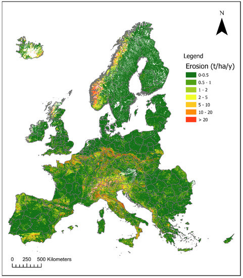
Figure 6.
Simulated long-term average erosion rates across Europe using the PESERA model.
SoilCare partners’ feedback on PESERA simulated erosion maps included for Spain that it seemed relatively low, compared to the national soil erosion map [84]. However, areas in the south show relatively high erosion in both maps. Belgium partners indicated that the relatively high erosion values for row crops like potato and sugar beet seemed valid, but that simulated erosion values for maize and vegetables, which have a wide spacing, were too low compared to their experience, especially when compared to simulated higher erosion in cereals. For Poland and Germany, simulated patterns of erosion were found to be plausible and matching e.g., the German national erosion map [85] with higher erosion in central Germany and very low to no erosion in the northern half of the country.
3.1.2. Baseline Long-Term SOC Stocks
Figure 7 shows the PESERA simulated maps of SOC stocks for Europe based on long-term average climate conditions (equilibrium phase model output). Overall estimates amount to 50 Gt, which is in line with estimates by Aagaard Kristensen et al. [77] (60 Gt), but somewhat higher than estimates of Yigini and Panagos [38] (38 Gt). The Nordic countries (Sweden, Finland) as well as the higher altitude areas clearly show higher SOC stocks (except where soil depth is shallow), while lower SOC stocks are simulated in for example inland Spain, parts of Italy, France and Eastern Europe. This coincides with the patterns of other SOC estimates (see Figures S12–S15). However, the SOC stock map based on the soil profile analytical database for Europe (SPADE; [77]; Figure S15), shows a slightly different pattern with lower SOC stock estimates for Sweden and parts of Finland, where our estimates show high SOC stocks. However, the intermediate stocks are similarly simulated to occur in the wet north-western Iberian Peninsula, the Massif Central in France and relatively low SOC stocks in the Norwegian mountain areas. Highest SOC stocks were simulated for forests, followed by grassland and shrubs. This matches estimates by other studies [38,39,77], although our estimates for grassland (11 Gt) are somewhat higher than those by Yigini and Panagos [38] (6.7 Gt). SOC stocks for fruit trees, olive groves and vineyard were estimated at around 60 t/ha on average across Europe, while the average SOC stocks for arable land across Europe was estimated at 43 t/ha or 5 Gt, which is lower than e.g., Lugato et al. [39] and Yigini and Panagos’ [38] estimates of 17.6 and 12.8 Gt respectively.
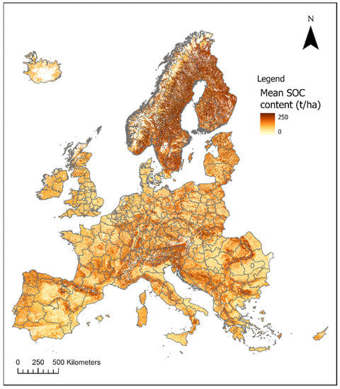
Figure 7.
Simulated long-term average SOC stocks across Europe using the PESERA model.
Calibration results for SOC stocks for the three countries and Crete for which the model was calibrated are shown in Table 4. Overall, results were close to the observed data, derived from the LUCAS database. However, for some crops or land uses it was difficult to simulate good values across climate zones. For example, while SOC stocks for potato cultivation were well estimated for Spain, values were too high for Belgium and Slovakia, but too low for Crete. For maize, values were overestimated for Belgium and Slovakia, but underestimated for Spain.
Table 4.
Calibrated (PESERA baseline long-term results) versus observed (LUCAS database) results for SOC (t/ha) for three countries and the Greek island of Crete in different climate zones. Note: X = crop does not occur. NA = not available.
SoilCare partners’ feedback on the PESERA calibrated SOC results indicated that they were in line with national estimates or maps (e.g., Belgium, Poland, Norway, Germany). For example, the German partners provided a German national map with organic matter [86], on which the spatial patterns were similar as those simulated by PESERA.
3.1.3. Calibration of the SICS
Figure 8 shows the simulated changes by the model for the individual SICS, compared with expected values from the literature. It should be noted that expected impacts on soil erosion were only found for cover crops, while the expected impacts on SOC were found for every SICS except compaction reduction; and that specific information for root crops and vegetables was less available than for cereals and permanent crops.
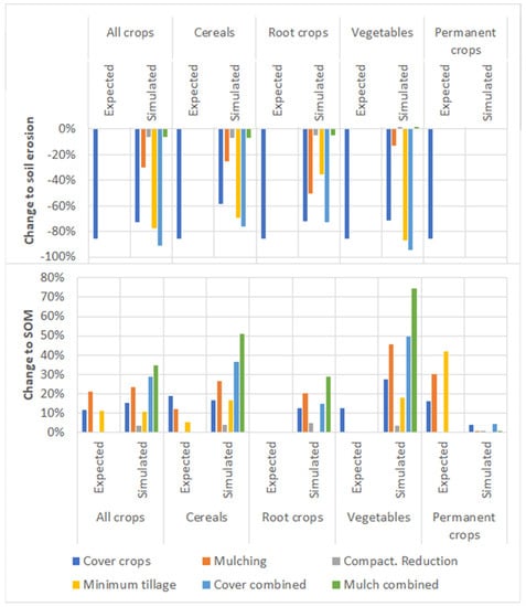
Figure 8.
Impact of different SICS (expected; based on literature review, see Table S7, and simulated with PESERA on a test dataset) on different types of crops, for erosion (top) and soil organic matter (bottom).
As can be seen, the simulated measures broadly followed what was expected from the literature in terms of erosion reduction and increase in SOC. When analysing per crop type, results for permanent crops tend not to be very good: no changes are simulated to erosion, because the baseline values were zero when using the test dataset; and changes to SOC are very limited. This indicates that the model is better adapted to simulate SOC changes for cereals than permanent crops. There is insufficient data to analyse model performance for root crops and vegetables.
In terms of impacts, PESERA simulates a small effect of compaction reduction when compared to other measures. For soil erosion control, mulching seems to have a limited effect in comparison to cover crops and minimum tillage; this results from the simulated wetter soil conditions when applying mulch, which increase biomass growth (and, indirectly, SOC) by limiting water stress, but also create the right conditions for more frequent runoff generation, counteracting beneficial soil protection effects. For SOC, mulching has a slightly larger benefit than cover crops or minimum tillage.
As for the combination SICS, both tend to lead to higher increases of SOC when compared with the individual components. For soil erosion, the combinations involving cover crops led to larger reductions than the individual components. However, the combined mulch approach had a very limited impact on soil erosion, despite the erosion decrease expected when applying the individual components. As both individual measures increase soil moisture, the wetter soil conditions and increased runoff counteract the soil protection effects of the measures. In short, results suggest that the combined cover crop approach appears to have a better balance between SOC increase and erosion control, while the combined mulching approach has larger increases of SOC at the expense of the effects on erosion control.
3.2. Simulated Results for SICS Scenarios
Figure 9 shows the simulated difference in annual erosion between year 2050 and current (2020) for the four scenarios. Note that differences in erosion are affected by differences in climate (e.g., wet months in certain years) as well as by the application of SICS. Some areas show a consistent slight increase in erosion; these are mainly the steep mountain areas (Alps, Pyrenees) and areas that receive a lot of rainfall (e.g., Norwegian coastal zone), where SICS are not applied, as they are covered by e.g., pasture or shrubland. However, for example in the central European Loess Belt, southern Spain and eastern Europe, erosion was simulated to increase in the RttB scenario, while it decreases in the CS scenario due to application of SICS. Overall, across Europe and taking all land uses into account, erosion was simulated to increase slightly for the RttB scenario (+1.3% compared to 2020), while a decrease was simulated for the UP, LS and CS scenarios (75, 79 and 59% respectively, compared to the 2020 situation). When taking only the arable and orchard (fruit trees, olive groves and vineyards) areas into account, where SICS are applied, simulated erosion decreased to 43, 49 and 6.6% (compared to 2020) for the UP, LS and CS scenarios respectively, which is an average decrease of about 1.5 t/ha/y in both the UP and LS scenarios, and 2.6 t/ha/y in the CS scenario. So, especially for the CS scenario, a large decrease in erosion was simulated, which is in line with the large reductions that were parameterised for e.g., cover crops (Figure 8). Simulated erosion maps for RttB 2020 and the four scenarios for 2050 are given in Supplementary Material S4.
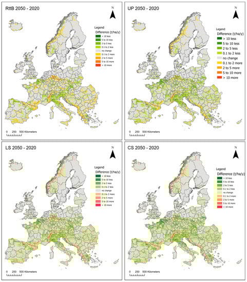
Figure 9.
Simulated difference in erosion (t/ha/y) between 2020 and 2050 for each scenario.
Figure 10 shows the simulated changes in SOC content for 2050, relative to the 2020 situation, for each of the four scenarios. All maps show both areas of decrease of SOC as well as areas of SOC increase. However, comparing between the scenarios, the results clearly show a more severe decrease in SOC for the RttB scenario, followed by UP, LS and CS scenarios. The average simulated SOC change across Europe, taking only the arable areas into account, was −23% for RttB, −4.5% for UP, −1.5% for LS and +22% for the CS scenario. This can also be seen in the maps (Figure 10): the CS scenario shows most increases in SOC content. For example, the arable areas in north-central Europe and north-central Spain that in the RttB show a strong decrease in SOC, turned into an increase in SOC in the CS scenario. This reflects the simulated SICS, where in CS all farmers apply a combination of minimum tillage, compaction reduction and either cover crops or mulching. In the UP scenario, all farmers apply only one type of SICS, while in the LS scenario, the application of SICS is mixed. Overall, it seems that, in terms of SOC content, the LS scenario leads to better results than the UP scenario, although local differences are likely greater in LS.
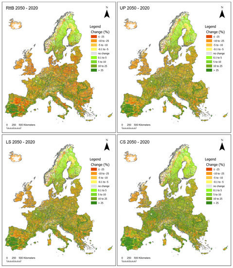
Figure 10.
Simulated change in SOC stock (%) between 2020 and 2050 for each scenario.
4. Discussion
Using the PESERA model, we simulated the effects of SICS on erosion and SOC stock changes across Europe, based on scenarios in which either no SICS were applied (RttB scenario; low sustainability level), or where a medium (UP scenario), high (CS scenario) or a mix of these three levels of sustainability was assumed (LS scenario). Comparing the effects of the simulated scenarios clearly shows that the application of a high level of sustainability, where all farmers apply a combination of SICS: minimum tillage, compaction reduction, and either cover crops (50%) or mulching (50%), results in highest and most widespread erosion reduction (Figure 9) and a shift from a continuous reduction in SOC stocks to an increase in SOC stocks (Figure 10). In general, our results imply that erosion can be quite well prevented by application of SICS (Figure 9), but less pronounced effects are simulated for SOC change. This is in line with often reported findings of relatively quick effects of measures on runoff and erosion while changing SOC is a slower process [87].
The scenarios we simulated contain a mix of measures, so direct comparison with other estimates is difficult. Panagos et al. [16,41] calculated the effect of the C (cover management) and P (conservation practices) factors. Panagos et al. [16] found that conservation tillage reduced the C-factor (and thus, indirectly erosion, if all other factors remain the same) by 17%, application of crop residues reduced the C-factor by 1.2% and cover crops by 1.3%. Note that these numbers are affected by the (relatively small) area where these practices were found to be applied and that large differences between countries were found [16]. Panagos et al. [41] estimated the P-factor (conservation practices), when including contouring, stone walls and grass margins, to be 0.9702 across Europe, meaning that erosion would be reduced by 3% (if all other factors remain the same). This factor has a wide spatial variation, being lower (i.e., more effective erosion protection) in for example Portugal, Spain and Belgium, due to a high number of stone walls and grass margins [41]. These findings are somewhat different than our results, as they do not include mulching. In our results, cover crops were estimated to reduce erosion significantly (also due to the calibration, see Figure 8). In a review study based on a large database of plot-scale erosion and runoff, including the effects of SWCTs (Soil and Water Conservation Techniques), Maetens et al. [18] found that overall, application of SWCTs reduced the exceedance probability for a soil loss tolerance of 5 t/ha/y and 12 t/ha/y by 14 and 12% respectively. The individual measures ranked in the order (more to less effective) of geotextiles, buffer strips, mulching, contour bunds, cover crops, conservation tillage and strip cropping [18]. They concluded that crop and vegetation management (mulching, cover crops) and mechanical measures (terraces, contour bunds) are more effective than soil management techniques (reduced tillage). While our study did not include mechanical measures in the scenarios, our results are in line with this as the CS scenario, where cover crops and mulching is always applied (in combination with minimum tillage and compaction reduction) is clearly more effective in reducing erosion than the UP scenario, where only half of the farmers applies mulching or cover crops. However, it should be noted that, for soil erosion, even a low intervention scenario (UP) can decrease erosion below 1 t/ha/y (Figure S20), which can be considered as a threshold for sustainability [88]. There is some variability between climate regions, and within them, between regions with different topography and soil types. Nevertheless, these results indicate that the UP scenario might be good enough for most agricultural crops in Europe; and that special attention, and stronger intervention measures, could focus on remaining crop types (pulses, root crops, etc.,) and on areas with higher erosion rates. The results from this work could be used as a first approach to define priority areas for different levels of intervention across Europe.
Similar as for erosion, also a direct comparison with other studies regarding the simulated changes in SOC stocks for our scenarios is difficult. Lugato et al. [49] simulated the effect of six management practices scenarios on possible carbon sequestration, including spatially explicit maps across Europe. They found that, besides conversion of arable land to grassland which showed the highest SOC sequestration rates, ley cropping systems and cover crops results in higher SOC sequestration than straw incorporation and reduced tillage, which is in line with our results. Aertsen et al. [47] investigated the effect of agroforestry, hedges along field boundaries, cover crops and no/low tillage on carbon sequestration for the EU27, concluding that agroforestry has the highest potential, and no spatial maps of Europe were presented. Bellassen et al. [48] did not include no-tillage practices, as they only redistribute SOC instead of sequestering it. They also state that cover crops have a substantial potential for carbon sequestration, but that the large-scale potential of other practices such as hedges and crop residues is probably limited. Lessmann et al. [89] combined global meta-analytical results with spatially explicit data on current management practices and potential areas for implementation of measures at a global scale and found that organic matter inputs led to highest mean SOC changes, followed by crop residue incorporation, reduced tillage and increased crop diversity [89].
While in general terms the simulated values and spatial patterns are in line with other studies, local experiments and observations might deviate. This is a difficulty in any upscaling to large (continental) scales. Factors that play a role include assumptions in the model (e.g., biomass and humus conversion factors are crop-specific, but not adaptable per region), lack of (spatially explicit) input data (for example the difficulty of deriving a reliable erodibility map) and scarcity of (observed; i.e., non-modelled) calibration and validation data across Europe [79], but see [18,77]. Therefore, the absolute values should be taken with caution, but a qualitative and comparative analysis over time and across Europe can be insightful.
In this study, we focussed on erosion, as one of the most important processes of land degradation [35] and SOC changes, as one of the most widely used and important indicators of soil health [32,33]. While these are important indicators, many other indicators and processes play a role in a healthy functioning soil [2,5]. However, simulation of all these functions together is almost impossible, especially at a large (e.g., EU) scale. A few studies are beginning to attempt this. For example, the Soil Navigator decision support system was developed to assess and optimise various soil functions [90] on farm scale, incorporating soil management strategies. This was applied to monitor multiple soil functions at 94 sites across 13 European countries [91]. Vrebos et al. [92] analysed and mapped four soil functions on agricultural lands across the EU. Borelli et al. [79] evaluated soil degradation in Europe, including both erosion and soil carbon fluxes using the WaTEM/SEDEM modelling approach, but did not include the effect of soil and water conservation measures.
Potential additions to the modelling approach that we simulated in this study, would be to include additional indicators, such as biomass growth and effects on yields. While this is possible in the current PESERA model, preliminary results showed some difficulties. However, coupling of PESERA with more sophisticated biomass and yield models such as QUEFTS [93] is feasible and ongoing. This would also allow to evaluate the effects of (changes in) nutrient supply to the crops within the SICS. Another improvement within the PESERA model is to enable the parameterisation/calibration in the SOC calculations in the model (e.g., the decomposition rates) to be both spatially and crop specific (they are at the moment only crop specific), for example by including a spatial map of annual decomposition rates in Europe [46]. In addition to this, land use change as well as climate change can be included in the modelling framework. Finally, while in this study we only evaluated the effects of SICS on environmental indictors, in a really comprehensive analysis and modelling framework, also socio-economic factors and indicators should be taken into account, such as economic profitability and adoption of measures. In the SoilCare project, an important finding was that although the CS scenario leads to highest impacts, the gross margin of SICS uptake under this scenario is negative in many NUTS-2 regions [24,65]. Moreover, note that the spatial allocation of SICS application (e.g., where which SICS was applied within the scenarios) was randomly allocated. Interestingly, overall, results of the UP scenario (medium sustainability level with one SICS applied in all arable lands) were close to those of the LS scenario (a mix of low (no measures), medium (one measure) and high (multiple measures) sustainability levels). However, the spatial variability in LS will be higher, meaning that areas with high erosion and low increase (or decrease) of SOC will be offset by other areas with high erosion reduction and increase in SOC stocks. To avoid this and reach land degradation neutrality (LDN, [94]), careful planning is required and in terms of the scenarios simulated here, regarding the allocation of measures there is room for improvement in the scenarios, for example to base the allocation of certain SICS in areas that need them most and/or are most suitable [95].
5. Conclusions
In this study we simulated the effects of Soil Improving Cropping Systems (SICS) on SOC stocks and erosion on EU scale using the PESERA model. Four scenarios with varying levels and combinations of SICS were simulated for the time period 2020–2050. We can conclude that, for both SOC stocks, as an indicator for soil health, and erosion, as indicator for land degradation, the scenario with the highest level of SICS, i.e., application of minimum tillage and compaction alleviation in combination with either mulch or cover crops, clearly decreases erosion levels substantially across Europe as well as turning a decreasing trend of SOC stocks (when no SICS are applied) into an increase in SOC stocks, on average across Europe. Scenarios with medium level of SICS application as well as a scenario that implemented a mix of no SICS, medium level and high level SICS throughout Europe showed a decrease in erosion, while SOC stocks remained at the current level.
Future improvements for this modelling study would include to add climate change and dynamic land use. Furthermore, SICS were now randomly allocated in the arable lands; further scenarios including a more targeted spatial allocation of the levels of SICS would be interesting to conduct.
Supplementary Materials
The following are available online at www.mdpi.com/article/10.3390/land11060943/s1. Supplementary material S1: Input data maps for PESERA (Figures S1–S11; Tables S1–S5). S2: EU scale maps of SOC stocks (Figures S12–S15) and erosion (Figures S16–S18) used for model evaluation and SOC calibration data (Table S6). S3: Literature used to compile effect of measures (Table S7); and S4: Simulated erosion maps for the baseline (2020; Figure S19), RttB, UP LS and CS 2050 (Figure S20).
Author Contributions
Conceptualisation, J.E.M.B., J.P.N., L.F. and H.v.D.; methodology, J.E.M.B., J.P.N., L.F., H.v.D. and R.V.; software, J.E.M.B., J.P.N., H.v.D. and R.V.; validation, J.E.M.B. and J.P.N.; formal analysis, J.E.M.B. and J.P.N.; investigation, J.E.M.B., J.P.N., L.F. and H.v.D.; resources, J.E.M.B., J.P.N., L.F. and H.v.D.; data curation, J.E.M.B. and J.P.N.; writing—original draft preparation, J.E.M.B. and J.P.N.; writing—review and editing, J.E.M.B., J.P.N., L.F. and H.v.D.; visualisation, J.E.M.B. and J.P.N.; project administration, J.E.M.B., J.P.N., L.F. and H.v.D.; funding acquisition, L.F. and H.v.D. All authors have read and agreed to the published version of the manuscript.
Funding
This research has received funding from the European Union’s Horizon 2020 research and innovation programme under grant agreement No 677407 (SoilCare project).
Institutional Review Board Statement
Not applicable in this study.
Informed Consent Statement
Not applicable in this study.
Data Availability Statement
The data presented in this study are available in the Figures in the paper and in the Supplementary Material S1–S4.
Acknowledgments
We acknowledge the E-OBS dataset from the EU-FP6 project UERRA (https://www.uerra.eu (accessed on 18 December 2020)) and the Copernicus Climate Change Service, and the data providers in the ECA&D project (https://www.ecad.eu (accessed on 18 December 2020)). We also acknowledge the feedback on preliminary model results by SoilCare partners, especially J. Stolte and R.J. Barneveld (NIBIO, Norway), M Tits and A. Elsen (Bodemkundige Dienst van Belgie, Belgium), P. Mayer-Gruner, E. Kandeler (University of Hohemheim, Germany), J. Cuevas, V. Pinillos (University of Almeria, Spain), M. Frac, J. Lipiec, B. Usowic (Institute of Agrophysics of the Polish Academy of Sciences, Poland); A. Berti, I. Piccoli (University of Padova, Italy); I. Calciu, O. Vizitiu (National Research and Development Institute for Soil Science, Agrochemistry and Environmental Protection, Romania), D. Alexakis, I. Tsanis (Technical University of Crete, Greece).
Conflicts of Interest
The authors declare no conflict of interest.
References
- Rust, N.A.; Jarvis, R.M.; Reed, M.S.; Cooper, J. Framing of sustainable agricultural practices by the farming press and its effect on adoption. Agric. Human Values 2021, 38, 753–765. [Google Scholar] [CrossRef]
- Bonfante, A.; Basile, A.; Bouma, J. Targeting the soil quality and soil health concepts when aiming for the United Nations Sustainable Development Goals and the EU Green Deal. SOIL 2020, 6, 453–466. [Google Scholar] [CrossRef]
- Lehmann, J.; Bossio, D.A.; Kögel-Knabner, I.; Rillig, M.C. The concept and future prospects of soil health. Nat. Rev. Earth Environ. 2020, 1, 544–553. [Google Scholar] [CrossRef]
- Yoder, D.C.; Jagadamma, S.; Singh, S.; Nouri, A.; Xu, S.; Saha, D.; Schaeffer, S.M.; Adotey, N.; Walker, F.R.; Lee, J.; et al. Soil health: Meaning, measurement, and value through a critical zone lens. J. Soil Water Conserv. 2022, 77, 88–99. [Google Scholar] [CrossRef]
- Bouma, J.; Montanarella, L.; Evanylo, G. The challenge for the soil science community to contribute to the implementation of the UN Sustainable Development Goals. Soil Use Manag. 2019, 35, 538–546. [Google Scholar] [CrossRef]
- European Commission. Farm to Fork Strategy—For a Fair, Healthy and Environmentally-Friendly Food System; European Commission: Brussels, Belgium, 2020. [Google Scholar]
- COM/2019/640. Final The European Green Deal. Available online: https://eur-lex.europa.eu/legal-content/EN/TXT/?qid=1576150542719&uri=COM%3A2019%3A640%3AFIN (accessed on 12 April 2022).
- Thomas, R.; Reed, M.; Clifton, K.; Appadurai, N.; Mills, A.; Zucca, C.; Kodsi, E.; Sircely, J.; Haddad, F.; Hagen, C.; et al. A framework for scaling sustainable land management options. L. Degrad. Dev. 2018, 29, 3272–3284. [Google Scholar] [CrossRef] [Green Version]
- Europarc Federation EU Farm to Fork. Available online: https://www.europarc.org/european-policy/farm-to-fork-protectes-areas/ (accessed on 12 April 2022).
- Veerman, C.; Pinto Correia, T.; Bastioli, C.; Biro, B.; Bouma, J.; Cienciala, E.; Emmett, B.; Frison, E.; Grand, A.; Hristov, L.; et al. Caring for Soil Is Caring for Life: Ensure 75% of Soils Are Healthy by 2030 for Food, People, nature and Climate: Report of the Mission Board for Soil Health and Food; European Commission: Brussels, Belgium, 2020. [Google Scholar] [CrossRef]
- World Overview of Conservation Approaches and Technologies (WOCAT). Where the Land Is Greener—Case Studies and Analysis of Soil and Water Conservation Initiatives Worldwide; Liniger, H., Critchley, W., Eds.; World Overview of Conservation Approaches and Technologies: Bern, Switserland, 2007. [Google Scholar]
- Kutter, T.; Louwagie, G.; Schuler, J.; Zander, P.; Helming, K.; Hecker, J.-M. Policy measures for agricultural soil conservation in the European Union and its member states: Policy review and classification. L. Degrad. Dev. 2011, 22, 18–31. [Google Scholar] [CrossRef]
- Lavergne, S.; Vanasse, A.; Thivierge, M.-N.; Halde, C. Using fall-seeded cover crop mixtures to enhance agroecosystem services: A review. Agrosystems, Geosci. Environ. 2021, 4, e20161. [Google Scholar] [CrossRef]
- Osipitan, O.A.; Dille, J.A.; Assefa, Y.; Knezevic, S.Z. Cover Crop for Early Season Weed Suppression in Crops: Systematic Review and Meta-Analysis. Agron. J. 2018, 110, 2211–2221. [Google Scholar] [CrossRef] [Green Version]
- Kathage, J.; Smit, B.; Janssens, B.; Haagsma, W.; Adrados, J.L. How much is policy driving the adoption of cover crops? Evidence from four EU regions. Land Use Policy 2022, 116, 106016. [Google Scholar] [CrossRef]
- Panagos, P.; Borrelli, P.; Meusburger, K.; Alewell, C.; Lugato, E.; Montanarella, L. Estimating the soil erosion cover-management factor at the European scale. Land Use Policy 2015, 48, 38–50. [Google Scholar] [CrossRef]
- Qin, W.; Hu, C.; Oenema, O. Soil mulching significantly enhances yields and water and nitrogen use efficiencies of maize and wheat: A meta-analysis. Sci. Rep. 2015, 5, 16210. [Google Scholar] [CrossRef] [PubMed]
- Maetens, W.; Poesen, J.; Vanmaercke, M. How effective are soil conservation techniques in reducing plot runoff and soil loss in Europe and the Mediterranean? Earth Sci. Rev. 2012, 115, 21–36. [Google Scholar] [CrossRef] [Green Version]
- Rodrigues, L.; Hardy, B.; Huyghebeart, B.; Fohrafellner, J.; Fornara, D.; Barančíková, G.; Bárcena, T.G.; De Boever, M.; Di Bene, C.; Feizienė, D.; et al. Achievable agricultural soil carbon sequestration across Europe from country-specific estimates. Glob. Chang. Biol. 2021, 27, 6363–6380. [Google Scholar] [CrossRef]
- Marshall, E.J.P.; Moonen, A.C. Field margins in northern Europe: Their functions and interactions with agriculture. Agric. Ecosyst. Environ. 2002, 89, 5–21. [Google Scholar] [CrossRef]
- Van Vooren, L.; Reubens, B.; Broekx, S.; De Frenne, P.; Nelissen, V.; Pardon, P.; Kris, V. Ecosystem service delivery of agri-environment measures: A synthesis for hedgerows and grass strips on arable land. Agric. Ecosyst. Environ. 2017, 244, 32–51. [Google Scholar] [CrossRef]
- Dorioz, J.M.; Wang, D.; Poulenard, J.; Trévisan, D. The effect of grass buffer strips on phosphorus dynamics—A critical review and synthesis as a basis for application in agricultural landscapes in France. Agric. Ecosyst. Environ. 2006, 117, 4–21. [Google Scholar] [CrossRef]
- Felsot, A.S.; Mitchell, J.K.; Kenimer, A.L. Assessment of Management Practices for Reducing Pesticide Runoff from Sloping Cropland in Illinois. J. Environ. Qual. 1990, 19, 539–545. [Google Scholar] [CrossRef]
- Hessel, R.; Wyseure, G.; Panagea, I.S.; Alaoui, A.; Reed, M.S.; van Delden, H.; Muro, M.; Mills, J.; Oenema, O.; Areal, F.; et al. Soil Improving cropping systems for sustainable and profitable farming in Europe. Land 2022, 11, 780. [Google Scholar] [CrossRef]
- Berhe, A.A. Chapter 3—Drivers of Soil Change. In Global Change and Forest Soils; Busse, M., Giardina, C.P., Morris, D.M., Page-Dumroese, D.S., Eds.; Elsevier: Amsterdam, The Netherlands, 2019; Volume 36, pp. 27–42. ISBN 0166-2481. [Google Scholar] [CrossRef]
- Lahmar, R. Adoption of conservation agriculture in Europe: Lessons of the KASSA project. Land Use Policy 2010, 27, 4–10. [Google Scholar] [CrossRef]
- Hijbeek, R.; Pronk, A.A.; van Ittersum, M.K.; Verhagen, A.; Ruysschaert, G.; Bijttebier, J.; Zavattaro, L.; Bechini, L.; Schlatter, N.; ten Berge, H.F.M. Use of organic inputs by arable farmers in six agro-ecological zones across Europe: Drivers and barriers. Agric. Ecosyst. Environ. 2019, 275, 42–53. [Google Scholar] [CrossRef]
- Montanarella, L. Trends in Land Degradation in Europe. In Climate and Land Degradation; Sivakumar, M.V.K., Ndiang’ui, N., Eds.; Springer: Berlin/Heidelberg, Germany, 2007; pp. 83–104. ISBN 978-3-540-72438-4. [Google Scholar] [CrossRef]
- Prăvălie, R.; Patriche, C.; Borrelli, P.; Panagos, P.; Roșca, B.; Dumitraşcu, M.; Nita, I.-A.; Săvulescu, I.; Birsan, M.-V.; Bandoc, G. Arable lands under the pressure of multiple land degradation processes. A global perspective. Environ. Res. 2021, 194, 110697. [Google Scholar] [CrossRef] [PubMed]
- Prăvălie, R. Exploring the multiple land degradation pathways across the planet. Earth Sci. Rev. 2021, 220, 103689. [Google Scholar] [CrossRef]
- Smiraglia, D.; Ceccarelli, T.; Bajocco, S.; Salvati, L.; Perini, L. Linking trajectories of land change, land degradation processes and ecosystem services. Environ. Res. 2016, 147, 590–600. [Google Scholar] [CrossRef] [PubMed]
- Bolinder, M.A.; Crotty, F.; Elsen, A.; Frac, M.; Kismányoky, T.; Lipiec, J.; Tits, M.; Tóth, Z.; Kätterer, T. The effect of crop residues, cover crops, manures and nitrogen fertilization on soil organic carbon changes in agroecosystems: A synthesis of reviews. Mitig. Adapt. Strateg. Glob. Chang. 2020, 25, 929–952. [Google Scholar] [CrossRef]
- Evenson, G.; Osterholz, W.R.; Shedekar, V.S.; King, K.; Mehan, S.; Kalcic, M. Representing soil health practice effects on soil properties and nutrient loss in a watershed-scale hydrologic model. J. Environ. Qual. 2022, 1–12. [Google Scholar] [CrossRef]
- Panagos, P.; Borrelli, P.; Poesen, J.; Ballabio, C.; Lugato, E.; Meusburger, K.; Montanarella, L.; Alewell, C. The new assessment of soil loss by water erosion in Europe. Environ. Sci. Policy 2015, 54, 438–447. [Google Scholar] [CrossRef]
- FAO. Soil Erosion: The Greatest Challenge to Sustainable Land Management; FAO: Rome, Italy, 2019. [Google Scholar]
- Van Delden, H.; Luja, P.; Engelen, G. Integration of multi-scale dynamic spatial models of socio-economic and physical processes for river basin management. Environ. Model. Softw. 2007, 22, 223–238. [Google Scholar] [CrossRef] [Green Version]
- Van Delden, H.; Stuczynski, T.; Ciaian, P.; Paracchini, M.; Hurkens, J.; Lopatka, A.; Shi, Y.; Calvo, S.; Van Vliet, J.; Vanhout, R.; et al. Integrated Assessment of Agricultural Policies with Dynamic Land Use Change Modelling. Ecol. Modell. 2010, 221, 2153–2166. [Google Scholar] [CrossRef]
- Yigini, Y.; Panagos, P. Assessment of soil organic carbon stocks under future climate and land cover changes in Europe. Sci. Total Environ. 2016, 557–558, 838–850. [Google Scholar] [CrossRef]
- Lugato, E.; Panagos, P.; Bampa, F.; Jones, A.; Montanarella, L. A new baseline of organic carbon stock in European agricultural soils using a modelling approach. Glob. Chang. Biol. 2014, 20, 313–326. [Google Scholar] [CrossRef] [PubMed]
- Morais, T.G.; Domingos, T.; Teixeira, R.F.M. A spatially explicit life cycle assessment midpoint indicator for soil quality in the European Union using soil organic carbon. Int. J. Life Cycle Assess. 2016, 21, 1076–1091. [Google Scholar] [CrossRef]
- Panagos, P.; Borrelli, P.; Meusburger, K.; van der Zanden, E.H.; Poesen, J.; Alewell, C. Modelling the effect of support practices (P-factor) on the reduction of soil erosion by water at European scale. Environ. Sci. Policy 2015, 51, 23–34. [Google Scholar] [CrossRef]
- Schulp, C.J.E.; Nabuurs, G.-J.; Verburg, P.H. Future carbon sequestration in Europe—Effects of land use change. Agric. Ecosyst. Environ. 2008, 127, 251–264. [Google Scholar] [CrossRef]
- Zaehle, S.; Bondeau, A.; Carter, T.R.; Cramer, W.; Erhard, M.; Prentice, I.C.; Reginster, I.; Rounsevell, M.D.A.; Sitch, S.; Smith, B.; et al. Projected Changes in Terrestrial Carbon Storage in Europe under Climate and Land-use Change, 1990–2100. Ecosystems 2007, 10, 380–401. [Google Scholar] [CrossRef]
- Smith, J.O.; Smith, P.; Wattenbach, M.; Zaehle, S.; Hiederer, R.; Jones, R.J.A.; Montanarella, L.; Rounsevell, M.D.A.; Reginster, I.; Ewert, F. Projected changes in mineral soil carbon of European croplands and grasslands, 1990–2080. Glob. Chang. Biol. 2005, 11, 2141–2152. [Google Scholar] [CrossRef]
- Frank, S.; Schmid, E.; Havlík, P.; Schneider, U.A.; Böttcher, H.; Balkovič, J.; Obersteiner, M. The dynamic soil organic carbon mitigation potential of European cropland. Glob. Environ. Chang. 2015, 35, 269–278. [Google Scholar] [CrossRef]
- Freibauer, A.; Rounsevell, M.D.A.; Smith, P.; Verhagen, J. Carbon sequestration in the agricultural soils of Europe. Geoderma 2004, 122, 1–23. [Google Scholar] [CrossRef]
- Aertsens, J.; De Nocker, L.; Gobin, A. Valuing the carbon sequestration potential for European agriculture. Land Use Policy 2013, 31, 584–594. [Google Scholar] [CrossRef]
- Bellassen, V.; Angers, D.; Kowalczewski, T.; Olesen, A. Soil carbon is the blind spot of European national GHG inventories. Nat. Clim. Chang. 2022, 12, 324–331. [Google Scholar] [CrossRef]
- Lugato, E.; Bampa, F.; Panagos, P.; Montanarella, L.; Jones, A. Potential carbon sequestration of European arable soils estimated by modelling a comprehensive set of management practices. Glob. Chang. Biol. 2014, 20, 3557–3567. [Google Scholar] [CrossRef] [PubMed] [Green Version]
- Panagea, I.S.; Berti, A.; Čermak, P.; Diels, J.; Elsen, A.; Kusá, H.; Piccoli, I.; Poesen, J.; Stoate, C.; Tits, M.; et al. Soil Water Retention as Affected by Management Induced Changes of Soil Organic Carbon: Analysis of Long-Term Experiments in Europe. Land 2021, 10, 1362. [Google Scholar] [CrossRef]
- Piccoli, I.; Seehusen, T.; Bussell, J.; Vizitu, O.; Calciu, I.; Berti, A.; Börjesson, G.; Kirchmann, H.; Kätterer, T.; Sartori, F.; et al. Opportunities for Mitigating Soil Compaction in Europe. Case Studies from the SoilCare Project Using Soil-Improving Cropping Systems. Land 2022, 11, 223. [Google Scholar] [CrossRef]
- Willett, W.; Rockström, J.; Loken, B.; Springmann, M.; Lang, T.; Vermeulen, S.; Garnett, T.; Tilman, D.; DeClerck, F.; Wood, A.; et al. Food in the Anthropocene: The EAT–Lancet Commission on healthy diets from sustainable food systems. Lancet 2019, 393, 447–492. [Google Scholar] [CrossRef]
- Kirkby, M.J.; Irvine, B.J.; Jones, R.J.A.; Govers, G.; Team, P. The PESERA coarse scale erosion model for Europe. I.—Model rationale and implementation. Eur. J. Soil Sci. 2008, 59, 1293–1306. [Google Scholar] [CrossRef]
- Abdelwahab, O.M.M.; Ricci, G.F.; De Girolamo, A.M.; Gentile, F. Modelling soil erosion in a Mediterranean watershed: Comparison between SWAT and AnnAGNPS models. Environ. Res. 2018, 166, 363–376. [Google Scholar] [CrossRef]
- Karamesouti, M.; Petropoulos, G.P.; Papanikolaou, I.D.; Kairis, O.; Kosmas, K. Erosion rate predictions from PESERA and RUSLE at a Mediterranean site before and after a wildfire: Comparison & implications. Geoderma 2016, 261, 44–58. [Google Scholar] [CrossRef]
- Berberoglu, S.; Cilek, A.; Kirkby, M.; Irvine, B.; Donmez, C. Spatial and temporal evaluation of soil erosion in Turkey under climate change scenarios using the Pan-European Soil Erosion Risk Assessment (PESERA) model. Environ. Monit. Assess. 2020, 192, 491. [Google Scholar] [CrossRef]
- Meusburger, K.; Konz, N.; Schaub, M.; Alewell, C. Soil erosion modelled with USLE and PESERA using QuickBird derived vegetation parameters in an alpine catchment. Int. J. Appl. Earth Obs. Geoinf. 2010, 12, 208–215. [Google Scholar] [CrossRef]
- Cornes, R.C.; van der Schrier, G.; van den Besselaar, E.J.M.; Jones, P.D. An Ensemble Version of the E-OBS Temperature and Precipitation Data Sets. J. Geophys. Res. Atmos. 2018, 123, 9391–9409. [Google Scholar] [CrossRef] [Green Version]
- Hargreaves, G.H.; Samani, Z.A. Reference Crop Evapotranspiration from Temperature. Appl. Eng. Agric. 1985, 1, 96–99. [Google Scholar] [CrossRef]
- Dosio, A. Projections of climate change indices of temperature and precipitation from an ensemble of bias-adjusted high-resolution EURO-CORDEX regional climate models. J. Geophys. Res. Atmos. 2016, 121, 5488–5511. [Google Scholar] [CrossRef]
- Panagos, P.; Meusburger, K.; Ballabio, C.; Borrelli, P.; Alewell, C. Soil erodibility in Europe: A high-resolution dataset based on LUCAS. Sci. Total Environ. 2014, 479–480, 189–200. [Google Scholar] [CrossRef] [PubMed]
- Abbaspour, K.; Ashraf Vaghefi, S. Harmonized World Soil Database in SWAT Format. PANGAEA 2019. [Google Scholar] [CrossRef]
- Andrews, T.; Gregory, J.M.; Webb, M.J.; Taylor, K.E. Forcing, feedbacks and climate sensitivity in CMIP5 coupled atmosphere-ocean climate models. Geophys. Res. Lett. 2012, 39, L09712. [Google Scholar] [CrossRef] [Green Version]
- Kotlarski, S.; Keuler, K.; Christensen, O.B.; Colette, A.; Déqué, M.; Gobiet, A.; Goergen, K.; Jacob, D.; Lüthi, D.; van Meijgaard, E.; et al. Regional climate modeling on European scales: A joint standard evaluation of the EURO-CORDEX RCM ensemble. Geosci. Model Dev. 2014, 7, 1297–1333. [Google Scholar] [CrossRef] [Green Version]
- Van Delden, H.; Fleskens, L.; Muro, M.; Tugran, T.; Vanhout, R.; Baartman, J.; Nunes, J.P.; Vanermen, I.; Salputra, G.; Verzandvoort, S.; et al. Report on the Potential for Applying Soil-Improving CS across Europe; Research Institute For Knowledge Systems: Maastricht, The Netherlands, 2021. [Google Scholar]
- Sacks, W.J.; Deryng, D.; Foley, J.A.; Ramankutty, N. Crop planting dates: An analysis of global patterns. Glob. Ecol. Biogeogr. 2010, 19, 607–620. [Google Scholar] [CrossRef]
- Rötzer, T.; Chmielewski, F.-M. Phenological maps of Europe. Clim. Res. 2001, 18, 249–257. [Google Scholar] [CrossRef]
- Brunel, S.; Suffert, M.; Petter, F.; Baker, R. Interface between pest risk science and policy: The EPPO perspective. NeoBiota 2013, 18, 9–23. [Google Scholar] [CrossRef]
- Gloning, P.; Estrella, N.; Menzel, A. The impacts of climate change on the winter hardiness zones of woody plants in Europe. Theor. Appl. Climatol. 2013, 113, 683–695. [Google Scholar] [CrossRef]
- Beck, H.E.; Zimmermann, N.E.; McVicar, T.R.; Vergopolan, N.; Berg, A.; Wood, E.F. Present and future Köppen-Geiger climate classification maps at 1-km resolution. Sci. Data 2018, 5, 180214. [Google Scholar] [CrossRef] [PubMed] [Green Version]
- Metzger, M.J.; Bunce, R.G.H.; Jongman, R.H.G.; Mücher, C.A.; Watkins, J.W. A climatic stratification of the environment of Europe. Glob. Ecol. Biogeogr. 2005, 14, 549–563. [Google Scholar] [CrossRef]
- Boons-Prins, E.R.; De Koning, G.H.J.; Van Diepen, C.A.; Penning de Vries, F.W.T. Crop-Specific Simulation Parameters for Yield Forecasting across the European Community; Wageningen University & Research: Wageningen, The Netherlands, 1993. [Google Scholar]
- Corlouer, E.; Gauffreteau, A.; Bouchet, A.-S.; Bissuel-Bélaygue, C.; Nesi, N.; Laperche, A. Envirotypes Based on Seed Yield Limiting Factors Allow to Tackle G × E Interactions. Agronomy 2019, 9, 798. [Google Scholar] [CrossRef] [Green Version]
- Irvine, B.J.; Kosmas, C. Pan-European Soil Erosion Risk Assessment—Deliverable 15: PESERA Users Manual; European Commission: Brussels, Belgium, 2003. [Google Scholar]
- De Brogniez, D.; Ballabio, C.; Stevens, A.; Jones, R.J.A.; Montanarella, L.; van Wesemael, B. A map of the topsoil organic carbon content of Europe generated by a generalized additive model. Eur. J. Soil Sci. 2015, 66, 121–134. [Google Scholar] [CrossRef]
- European Environmental Agency Variations in Topsoil Organic Carbon Content across Europe. Available online: https://www.eea.europa.eu/data-and-maps/figures/variations-in-topsoil-organic-carbon (accessed on 30 November 2020).
- Aagaard Kristensen, J.; Balstrøm, T.; Jones, R.J.A.; Jones, A.; Montanarella, L.; Panagos, P.; Breuning-Madsen, H. Development of a harmonised soil profile analytical database for Europe: A resource for supporting regional soil management. SOIL 2019, 5, 289–301. [Google Scholar] [CrossRef] [Green Version]
- Cerdan, O.; Govers, G.; Le Bissonnais, Y.; Van Oost, K.; Poesen, J.; Saby, N.; Gobin, A.; Vacca, A.; Quinton, J.; Auerswald, K.; et al. Rates and spatial variations of soil erosion in Europe: A study based on erosion plot data. Geomorphology 2010, 122, 167–177. [Google Scholar] [CrossRef]
- Borrelli, P.; Van Oost, K.; Meusburger, K.; Alewell, C.; Lugato, E.; Panagos, P. A step towards a holistic assessment of soil degradation in Europe: Coupling on-site erosion with sediment transfer and carbon fluxes. Environ. Res. 2018, 161, 291–298. [Google Scholar] [CrossRef]
- Rietra, R.; Heinen, M.; Oenema, O. A Review of Crop Husbandry and Soil Management Practices Using Meta-Analysis Studies: Towards Soil-Improving Cropping Systems. Land 2022, 11, 255. [Google Scholar] [CrossRef]
- Jian, J.; Du, X.; Reiter, M.S.; Stewart, R.D. A meta-analysis of global cropland soil carbon changes due to cover cropping. Soil Biol. Biochem. 2020, 143, 107735. [Google Scholar] [CrossRef]
- Luo, Z.; Wang, E.; Sun, O.J. Can no-tillage stimulate carbon sequestration in agricultural soils? A meta-analysis of paired experiments. Agric. Ecosyst. Environ. 2010, 139, 224–231. [Google Scholar] [CrossRef]
- Hamza, M.A.; Anderson, W.K. Soil compaction in cropping systems: A review of the nature, causes and possible solutions. Soil Tillage Res. 2005, 82, 121–145. [Google Scholar] [CrossRef]
- Ministerio Para la Transicion Ecologica y el reto Demografico Inventario Nacional de Erosion de Suelos. Available online: https://www.miteco.gob.es/es/biodiversidad/temas/inventarios-nacionales/inventario-nacional-erosion-suelos/estado_actual.aspx (accessed on 12 April 2022).
- Umwelt Bundesamt Mittlerer Landjaehriger Sedimenteintrag in Die Oberflaechengewaesser Durch Wassererosion. Available online: https://www.umweltbundesamt.de/themen/boden-landwirtschaft/bodenbelastungen/bodenerosion/bodenerosion-durch-wasser#schutz-vor-erosion-ist-auch-gewasserschutz (accessed on 12 April 2022).
- BGR Gehalte an Organischer Substanz in Oberboeden Deutschlands 1:1,000,000. Available online: https://www.bgr.bund.de/DE/Themen/Boden/Bilder/Bod_Humuskarte_g.jpg?__blob=normal&v=3 (accessed on 12 April 2022).
- Poeplau, C.; Don, A. Carbon sequestration in agricultural soils via cultivation of cover crops—A meta-analysis. Agric. Ecosyst. Environ. 2015, 200, 33–41. [Google Scholar] [CrossRef]
- Verheijen, F.G.A.; Jones, R.J.A.; Rickson, R.J.; Smith, C.J.; Bastos, A.C.; Nunes, J.P.; Keizer, J.J. Concise overview of European soil erosion research and evaluation. Acta Agric. Scand. Sect. B Soil Plant Sci. 2012, 62, 185–190. [Google Scholar] [CrossRef]
- Lessmann, M.; Ros, G.H.; Young, M.D.; de Vries, W. Global variation in soil carbon sequestration potential through improved cropland management. Glob. Chang. Biol. 2022, 28, 1162–1177. [Google Scholar] [CrossRef] [PubMed]
- Debeljak, M.; Trajanov, A.; Kuzmanovski, V.; Schröder, J.; Sandén, T.; Spiegel, H.; Wall, D.P.; de Broek, M.; Rutgers, M.; Bampa, F.; et al. A Field-Scale Decision Support System for Assessment and Management of Soil Functions. Front. Environ. Sci. 2019, 7, 115. [Google Scholar] [CrossRef] [Green Version]
- Zwetsloot, M.J.; van Leeuwen, J.; Hemerik, L.; Martens, H.; Simó Josa, I.; de Broek, M.; Debeljak, M.; Rutgers, M.; Sandén, T.; Wall, D.P.; et al. Soil multifunctionality: Synergies and trade-offs across European climatic zones and land uses. Eur. J. Soil Sci. 2021, 72, 1640–1654. [Google Scholar] [CrossRef]
- Vrebos, D.; Jones, A.; Lugato, E.; O’Sullivan, L.; Schulte, R.; Staes, J.; Meire, P. Spatial evaluation and trade-off analysis of soil functions through Bayesian networks. Eur. J. Soil Sci. 2021, 72, 1575–1589. [Google Scholar] [CrossRef]
- Sattari, S.Z.; van Ittersum, M.K.; Bouwman, A.F.; Smit, A.L.; Janssen, B.H. Crop yield response to soil fertility and N, P, K inputs in different environments: Testing and improving the QUEFTS model. F. Crop. Res. 2014, 157, 35–46. [Google Scholar] [CrossRef]
- UNCCD Land Degradation Neutrality. Available online: https://www.unccd.int/land-and-life/land-degradation-neutrality/overview#:~:text=WedefineLDNas“a,andspatialscalesandecosystems.” (accessed on 12 April 2022).
- Van Delden, H.; Fleskens, L.; Vanhout, R.; Nunes, J.P.; Baartman, J.; Lesschen, J.P.; Verzandvoort, S.; Hessel, R.; All Study Site Partners. Report on the Integration and Synthesis of Study Site Results and Their Potential for Upscaling; Wageningen University & Research: Wageningen, The Netherlands, 2021. [Google Scholar]
Publisher’s Note: MDPI stays neutral with regard to jurisdictional claims in published maps and institutional affiliations. |
© 2022 by the authors. Licensee MDPI, Basel, Switzerland. This article is an open access article distributed under the terms and conditions of the Creative Commons Attribution (CC BY) license (https://creativecommons.org/licenses/by/4.0/).