Factors Influencing the Coupling of the Development of Rural Urbanization and Rural Finance: Evidence from Rural China

Abstract

This study empirically analyzes factors influencing the coupling and coordinated development of rural urbanization and rural finance. For this purpose, the study employs the coupling degree model and develops a panel quantile model to estimate the coupling degree and coupling coordination degree of rural urbanization and rural finance. Accordingly, the study presents panel data comprising 31 provinces, municipalities, and autonomous regions in China from 2010 to 2019. The empirical results reveal that the coupling degree of rural urbanization and rural finance is relatively low in most study areas. This result suggests that rural urbanization and rural financial development in most provinces in China have not exhibited coordinated development. Further, the results reveal that urban population density negatively affects the coupling and coordination degree of rural urbanization and rural finance. Moreover, the effects of urban population density are more significant in areas with a low coupling coordination degree compared with those with a higher coupling coordination degree. An increase in the quantile gradually decreases the effect of the proportion of educational expenditure to GDP on the degree of rural urbanization and rural financial coupling coordination. However, the effect of financial development efficiency increases accordingly. The per capita GDP, per capita fiscal expenditure, and per capita built-up area significantly affect all the quantiles, indicating a positive correlation. This correlation can promote the coupling and coordinated development of rural urbanization and rural finance. In areas with a low coupling coordination degree, the financial development scale significantly positively affects the coupling coordination degree of rural urbanization and rural finance. In areas with a high coupling coordination degree, the financial development scale significantly negatively correlates with the coupling coordination degree. In addition, a positive correlation exists between the financial development structure and the coupling coordination degree of rural urbanization and rural finance.

1. Introduction

The continuous development of urbanization in China has gradually reduced the size of the rural population and has resulted in the emergence of a large number of ‘hollow villages’; at the same time, a large number of people may continue to reside in rural areas for a long time [1]. Considering the rural residents’ benefit, China’s 14th Five-Year Plan (2021–2025) has clearly proposed a two-wheel-drive strategy of new urbanization and rural revitalization [2]. Under the new development pattern, with domestic circulation as the main body and the dual circulation of domestic and international circulations promoting each other, the government drives the construction of modern metropolitan areas in development advantage areas; on the other hand, the state attaches great importance to rural revitalization. Between urbanization and rural revitalization, the term ‘rural urbanization’ has entered people’s parlance [1]. As the core of a modern economy, finance plays a crucial role in a country’s major development strategy [3]. The development of rural urbanization requires a large amount of capital investment. Thus, a perfect rural financial system is urgently required to meet the financial needs of rural urbanization to ensure the key role of funds in resource allocation and financial communication. Similarly, the development of rural finance requires a good social environment to ensure that the promotion of rural urbanization can provide a guarantee for the development of rural finance. Therefore, one of the urgent problems to be solved in the current rural economic development is the coordination of the development of rural urbanization and rural finance.

Recently, scholars have conducted multiple studies on the relation between urbanization and finance. However, research on the coupling and coordination relationships between rural urbanization and rural finance has been relatively scarce. Furthermore, factors determining the coupling and coordinated development of rural urbanization and rural finance have not been discussed. Therefore, this study focuses on the coupling relationship between rural urbanization and rural finance. Moreover, the study empirically reveals factors determining the coordinated development of rural urbanization and rural finance by developing a panel quantile model. We tested the effects of urban population density (UPD), per capita GDP (PCGDP), per capita disposable income of rural residents (PCDIRR), per capita fiscal expenditure (PCFE), the proportion of educational expenditure to GDP (PEEGDP), per capita built-up area (PCBA), financial development efficiency (FDE), financial development scale (FDSC), and financial development structure (FDST) on the coupling coordination degree (CCD) of rural urbanization and rural finance.

The paper is structured as follows: The second section reviews the research results of domestic and foreign scholars on rural urbanization and rural finance. The third section employs the entropy evaluation method to construct comprehensive evaluation systems of rural urbanization and rural finance. In the fourth section, the coupling coordination model is used to analyze the coupling coordination degree between the comprehensive evaluation systems of rural urbanization and those of rural finance. In the fifth section, the panel quantile model is constructed to examine factors determining the coupling development of rural urbanization and rural finance. The sixth section presents the conclusion and policy recommendations.

2. Literature Review

One of the urgent problems to be solved in current rural economic development is determining ways to promote the coordinated development of rural urbanization and rural finance. Accordingly, numerous scholars have begun exploring the interactive relation between rural urbanization and rural finance. Therefore, numerous studies have been conducted on rural urbanization and rural finance, and fruitful research results have been achieved. The existing literature discusses the problems involved in various aspects of the process of rural urbanization, including policy implementation [4,5], land-use variation [6], agricultural land transfer [7], agriculture issues [8], social inequality [9], and industrial adjustment [10]. In addition, several studies have focused on rural finance. For instance, these studies have explored digital credit scoring in rural finance [11], the effect of rural finance on rural industrial integration [12], and agricultural technology adoption [13]. Scholars have also studied China’s rural finance from the perspective of political economy [14,15], rural financial problems in small farms [16], and the inclusive reform of rural finance [17]. In sum, previous scholars have achieved fruitful results in their research on rural urbanization and rural finance, and those are of great reference significance to this paper.

However, the existing literature focuses less on the interaction between rural urbanization and rural finance in China. It mainly focuses on two aspects: First, research was to unidirectionally examine the effect of rural financial development on the urbanization construction in China’s rural areas. Tang and Zhang [18] adopted a vector autoregressive model (VAR) to empirically analyze the role of rural financial development in China’s rural urbanization construction. The empirical results revealed that the increase of rural financial scale and structural adjustment slightly affected rural urbanization, and the improvement of rural financial efficiency had a higher contribution rate to the effect on rural urbanization. Ding and Duan [19] examined the manner in which rural finance accelerated the development of urbanization in rural China. They believed that the rapid development of urbanization in China’s rural areas should be promoted by correcting the service functions of rural financial institutions and establishing a diversified rural financial system. Yan and Yang [20] explicated the driving role of rural finance in the development of rural urbanization in China, focusing on the four aspects of necessity, specific contents, problems, and suggestions of strategies for rural finance to support urbanization construction. The second research focus was on the development of rural finance in the process of the urbanization of rural China. Yu and Kong [21] examined environmental variation and the corresponding reform of rural finance in the process of rural urbanization. The specific explanation of environmental variation is that the closed and close traditional social relation network is gradually disintegrating, and the corresponding rural financial reform is to rebuild the rural social relation network and enhance the degree of rural organization. Ran and Ran [22] explored the manner in which rural financial institutions in different regions should choose appropriate organizational forms when facing different levels of rural urbanization.

In the existing literature, scholars have recognized the positive role of rural financial development in promoting rural urbanization in China. However, research on the relation between rural urbanization and financial development is mainly unidirectional. Furthermore, quantitative research on the mutual interaction between rural urbanization and financial development is relatively scarce and has not yet involved the analysis of the relationship between the two systems. Presently, research on the coupling and coordinated relation of urbanization and finance in China has mainly focused on the regions of a single province [23,24], multiple provinces [25], and multiple urban agglomerations [26]. No scholar has explored the coupling and coordinated development of rural urbanization and rural finance in China at the national level. Based on this situation, this study considers rural areas in China as the research object, constructs comprehensive evaluation index systems of rural urbanization and rural finance, and measures the degree of coupling and coordination between the two by using the coupling and coordination degree model. Besides taking the coupling and coordination degree of rural urbanization and rural finance as the dependent variable, this study considers variables with larger weights in the rural urbanization index and rural finance index as driving factors to reveal factors influencing the coordinated development of rural urbanization and rural finance in China, thereby providing a scientific reference for the coordinated and sustainable development of the two systems.

3. Comprehensive Evaluation of Rural Urbanization and Rural Financial Development

3.1. Data Sources

This study selected panel data comprising 31 provinces, municipalities, and autonomous regions in China (Figure 1) from 2010 to 2019. The data were obtained from different yearbooks published from 2011 to 2020, including The China Statistical Yearbook, The Almanac of China’s Finance and Banking, The Finance Yearbook of China, and The China Rural Statistical Yearbook, while part of the data was obtained from the National Bureau of Statistics of China website.

3.2. Construction of Index System for Rural Urbanization

On the premise of following the principles of science—measurability, systematicness, and accessibility, this study developed a comprehensive index system for rural urbanization based on five aspects [24,25,27,28,29]: economic urbanization, population urbanization, social urbanization, spatial urbanization, and environmental urbanization. Economic urbanization was mainly measured at the economic, investment, and fiscal levels. The economic level included both the per capita GDP (yuan) and the per capita disposable income of rural residents. The investment level was mainly measured by the per capita fixed asset investment, and the fiscal level was mainly measured by the per capita financial expenditure. Population urbanization mainly reflects the level of urbanization development. Population urbanization in this study was measured considering three aspects: population size, population quality, and employment. First, the population size was mainly measured through the proportion of urban population and the density of urban population (person/km²). Second, the quality of the population was measured in terms of the number of college students per 100,000 people. Third, employment level was measured using the proportion of secondary and tertiary employees (%) in total employment. Social urbanization included two aspects: education level and living standard. The level of education was mainly reflected by the proportion of educational expenditure to GDP (%). The living standard was mainly measured by the per capita consumption of rural residents. Spatial urbanization included three aspects: urban scale, living space, and afforestation level. The scale of urban areas was mainly measured by the proportion of built-up area to the total urban area, the living space was measured by the built-up area per capita (m²) and the area of park greenspace per capita (m²), and the afforestation level was measured by the area of park greenspace per capita (m²). Environmental urbanization indicates the protection of the environment and reflects the quality of the environment. It mainly includes three aspects: the harmless disposal rate (%) of urban household waste, the green coverage (%) of built-up areas, and the amount of household waste disposal (10,000 tons). The comprehensive index system of rural urbanization is presented in

Table 1. Comprehensive Index System of Rural Urbanization.

Comprehensive Index	Sub- Layers	Index	No.	Index Definition	Attribute
Rural urbanization	Economic urbanization	Economic level	1	Per capita GDP (PCGDP) (yuan)	+
			2	Per capita disposable income of rural residents (PCDIR)	+
		Investment level	3	Per capita investment in fixed assets	+
		Fiscal level	4	Per capita fiscal expenditure (PCFE)	+
	Population urbanization	Population size	5	Urban population density (UPD) (person/km2)	+
			6	Proportion of urban population	+
		Population quality	7	Number of college students per 100,000 people	+
		Economic group	8	Proportion of employees in secondary and tertiary industries in total employment (%)	+
	Social urbanization	Educational level	9	Proportion of educational expenditure to GDP (PEEGDP) (%)	+
		Living standard	10	Per capita consumption of rural residents	+
	Spatial urbanization	Urban scale	11	Proportion of built-up area in total urban area	+
		Living space	12	Per capita built-up area (PCBA) (m2)	+
			13	Urban road area per capita (m2)	+
		Afforestation level	14	Per capita park and greenspace area(m2)	+
	Environmental urbanization	Environmental quality	15	Harmless disposal rate (%) of urban household waste	+
			16	Amount of household waste disposal (10,000 tons)	+
			17	Green coverage (%) of built-up areas	+

.

3.3. Construction of a Rural Financial Index System

For the description of rural finance, scholars have conducted in-depth discussions and have proposed many indices for measurement. Hu and Chen [30] measured rural finance via financial development scale and financial development efficiency. Refs. [31,32,33,34] believed that, in addition to the scale and efficiency of financial development, rural financial development structure should be introduced to measure rural financial development. Therefore, based on previous studies, and combined with the availability and effectiveness of indices, this study selected the scale, efficiency, and structure of financial development as indices to measure rural financial development.

Financial development scale (FDSC). The McKinnon and Goldsmith indices are widely used to measure the scale of financial development. Specifically, the McKinnon index is measured via the ratio of broad currency (M2) to gross domestic product (GDP). The Goldsmith index is measured via the ratio of total rural deposits and loans to the total rural GDP. However, some scholars have held a negative attitude towards the McKinnon index. For instance, Hu and Chen [30] believed that the McKinnon index does not adequately reflect the actual situation of rural finance in China. Therefore, some scholars have employed the Goldsmith index to describe the scale of financial development. For instance, Refs. [35,36,37] selected the ratio of deposits and loans of financial institutions to nominal agricultural GDP as a description tool. Considering the research results of previous scholars and the research content of this paper, the Goldsmith index was chosen to describe the scale of financial development. In this study, rural deposits were defined as the sum of peasant household savings deposits and agricultural deposits, and rural loans were defined as the sum of agricultural loans and loans for township enterprises. Rural GDP represented the sum of the total agricultural output value and the added value of township enterprises. Since the rural township enterprises mainly conduct agriculture, forestry, animal husbandry, and fishery, the value added of township enterprises in this study was replaced by the value added of agriculture, forestry, animal husbandry, and fishery.

Financial development efficiency (FDE). The efficiency of financial development reflects the speed of financial development. Most scholars have defined financial development efficiency as the efficiency of financial intermediaries in converting savings into loans. Ding et al. [38] utilized the ratio of rural loan balance to rural deposit balance to measure the ability of rural financial institutions to convert deposits into loans. Moreover, Refs. [34,39,40] chose the ratio of deposit to loan to measure the financial development efficiency of rural credit cooperatives. Similarly, this study measured financial development efficiency through the ability of rural financial institutions to convert deposits into loans. Furthermore, the study used the ratio of rural deposits to rural loans to describe the ability of rural financial institutions to convert deposits into loans. The faster the rural financial institutions convert deposits into loans, the higher the financial development efficiency, and vice versa.

Financial development structure (FDST). Financial development structure reflects the distribution structure of rural financial funds and resources. Guo and Wang (2012) [41] examined the support of rural finance to the development of rural economy and used the balance of loans of township enterprises and rural loans to measure the structure of rural financial development. In measuring rural financial maturity, Refs. [42,43,44] selected the ratio of township enterprise loans to rural loans as an indicator to describe the structure of rural financial development. Accordingly, this study adopted the ratio of township enterprise loans to rural loans as the index of rural financial development structure.

3.4. Comprehensive Evaluation Method

This study employed the entropy evaluation method to calculate weight. In this objective weighting method, the degree of difference between the evaluation index values is used to determine the coefficient. In this process, the deviation caused by subjective factors is avoided, and the importance of each index is objectively reflected in the comprehensive index system. Therefore, this study applied the aforementioned method to measure the index weight of rural urbanization development.

Notably, before calculating the entropic value, these indices were required to be dimensionless so as to eliminate the influence of difference caused by type and dimension inconsistency among the evaluation indices. Normalization was used to standardize each index.

The normalization process of the original data was as follows:

(1)

Positive index treatment method:

$$X_{ij}=\left[\frac{x_{ij}-\min x_{ij}}{\max x_{ij}-\min x_{ij}}\right]\times 100\%$$

(1)

(2)

Negative index treatment method:

$$X_{ij}=\left[\frac{\max x_{ij}-x_{ij}}{\max x_{ij}-\min x_{ij}}\right]\times 100\%$$

(2)

The comprehensive evaluation process was as follows:

In Step 1, the index j was calculated. The proportion of scheme i to the index is indicated in Equation (3):

$$p_{ij}=\frac{X_{ij}}{{\displaystyle \sum _{i=1}^n{X}_{ij}}},(j=1,2,\cdots ,n)$$

(3)

In Step 2, the entropy of the index was calculated. Furthermore, $p_{ij}$ calculated by Equation (3) was used to calculate the entropy of the index j, as indicated in Equation (4):

$$e_j=-K\ast {\displaystyle \sum _{i=1}^n{p}_{ij}}\ln (p_{ij})$$

(4)

where $K>0$, ln is a natural logarithm, and $e_j\ge 0$. In Equation (4), the value of K is shown to be related to the sample size n, $K=\frac{1}{\ln (n)}$, where n denotes the number of samples.

The third step was to calculate the coefficient of variation. Equation (4) was used to calculate the entropy $e_j$ of index j and the coefficient of variation of item j, as indicated in Equation (5):

$$g_j=1-e_j$$

(5)

The magnitude of the coefficient of variation determines the importance of the index: the larger the coefficient of variation, the more important the index. If the coefficient of variation is small, the index is not that important.

Step 4 was to calculate the index weight. The coefficient of variation of index calculated by Equation (5) calculates the weight of the index as presented in Equation (6):

$$W_j=\frac{g_j}{{\displaystyle \sum _{j=1}^n{g}_j}},\left(j=1,2,\cdots ,n\right)$$

(6)

Step 5 was to calculate the comprehensive score. First, the index weight was calculated. Thereafter, the sum of the product of the score of each index and its corresponding weight were used to obtain the comprehensive evaluation value, as indicated in Equation (7):

$$S_i={\displaystyle \sum _{j=1}^n{W}_j}{P}_{ij},\left(i=1,2,\cdots ,n\right)$$

(7)

By the entropy method, we calculated the index weights as shown in

Table 2. Comprehensive Index Weight of Rural Urbanization.

Sub- Layers	Index	No.	Index Definition	Weight
Economic urbanization	Economic level	1	Per capita GDP (PCGDP) (yuan)	0.04
		2	Per capita disposable income of rural residents (PCDIR)	0.05
	Investment level	3	Per capita investment in fixed assets	0.05
	Fiscal level	4	Per capita fiscal expenditure (PCFE)	0.01
Population urbanization	Population size	5	Urban population density (UPD) (person/km2)	0.28
		6	Proportion of urban population	0.03
	Population quality	7	Number of college students per 100,000 people	0.03
	Economics group	8	Proportion of employees in secondary and tertiary industries in total employment (%)	0.05
Social urbanization	Educational level	9	Proportion of educational expenditure to GDP (PEEGDP) (%)	0.09
	Living standard	10	Per capita consumption of rural residents	0.08
Spatial urbanization	Urban scale	11	Proportion of built-up area in total urban area	0.04
	Living space	12	Per capita built-up area (PCBA) (m2)	0.08
		13	Urban road area per capita (m2)	0.03
	Afforestation level	14	Per capita park and greenspace area(m2)	0.03
Environmental urbanization	Environmental quality	15	Harmless disposal rate (%) of urban household waste	0.02
		16	Amount of household waste disposal (10,000 tons)	0.08
		17	Green coverage (%) of built-up areas	0.01

.

3.5. Comprehensive Evaluation Results of Rural Urbanization and Rural Financial Development

3.5.1. Comprehensive Evaluation Results of Urbanization Development in Rural Areas

The comprehensive evaluation method was used to calculate the comprehensive score of rural urbanization in China from 2010 to 2019 (the comprehensive evaluation index of rural finance). The comprehensive evaluation index of rural urbanization for each province, municipality, and autonomous region in China has been averaged and ranked, as presented in

Table 3. Average Comprehensive Evaluation Index of Rural Urbanization.

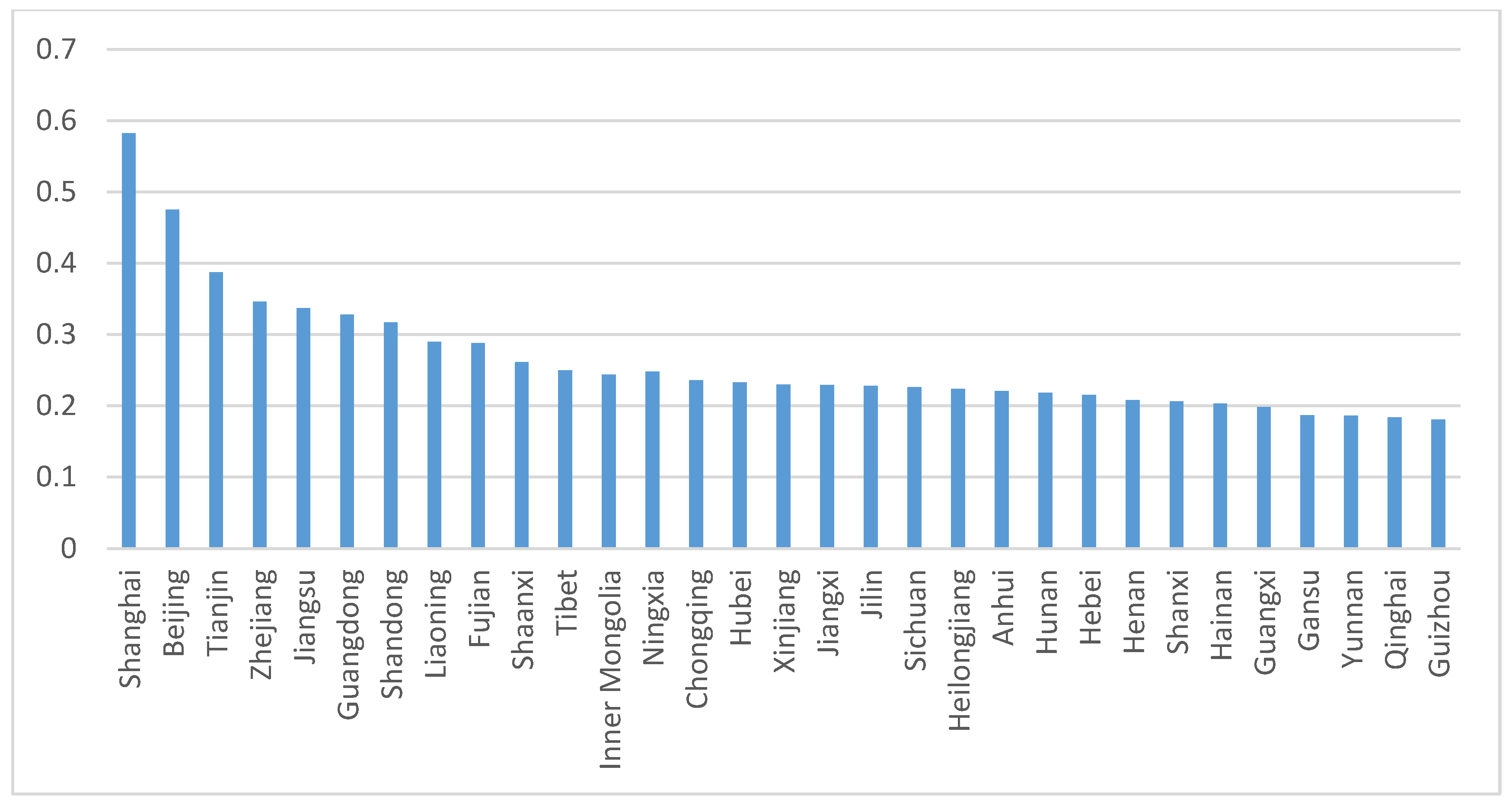
Region	Average Comprehensive Evaluation Index	Region	Average Comprehensive Evaluation Index	Region	Average Comprehensive Evaluation Index	Region	Average Comprehensive Evaluation Index
Shanghai	0.582	Fujian	0.288	Jiangxi	0.229	Shanxi	0.206
Beijing	0.475	Shaanxi	0.261	Jilin	0.228	Hainan	0.203
Tianjin	0.387	Tibet	0.250	Sichuan	0.226	Guangxi	0.198
Zhejiang	0.346	Inner Mongolia	0.244	Heilongjiang	0.224	Gansu	0.187
Jiangsu	0.337	Ningxia	0.248	Anhui	0.221	Yunnan	0.186
Guangdong	0.328	Chongqing	0.236	Hunan	0.218	Qinghai	0.184
Shandong	0.317	Hubei	0.233	Hebei	0.215	Guizhou	0.181
Liaoning	0.290	Xinjiang	0.230	Henan	0.208

.

The average comprehensive evaluation index of rural urbanization in China’s provinces, municipalities, and autonomous regions from 2010 to 2019 is depicted using a histogram, as presented in Figure 2. Figure 2 indicates that the average comprehensive evaluation index of rural urbanization in most areas was 0.2–0.3. Shanghai had the highest average comprehensive index, and the comprehensive evaluation index was 0.582. This occurred because Shanghai is economically developed; many rural areas have been urbanized, and the proportion of urban population is much larger than that of other provinces. Beijing ranked second, with an average comprehensive index of 0.475. As the center of Chinese economy, politics, and culture, Beijing is the most quickly urbanizing area in China. Gansu, Yunnan, Qinghai, and Guizhou, whose average index values were all below 0.19, marked the lowest comprehensive evaluation indices of rural urbanization. This was because these areas are located in arid and plateau areas in Western China, with inconvenient transportation and backward economies. Moreover, their urbanization seriously lag behind by the coastal and central areas in China.

3.5.2. Comprehensive Evaluation Results of Rural Financial Development

The method of calculating the comprehensive score of the rural financial system resembles that of the rural urbanization system. The weights of the financial development scale, financial development efficiency, and financial development structure were 0.531, 0.096, and 0.373, respectively. Clearly, the largest proportion of rural financial development was the scale of financial development. In this study, the scale of financial development was measured by the ratio of total rural deposits and loans to rural GDP, implying that the total rural finance, deposits, and loans were closely related to rural GDP. First, the weight of each index of rural finance was calculated by adopting the entropy evaluation value method. Thereafter, the comprehensive score of rural finance from 2010 to 2019 was calculated by the weight, that is, the comprehensive evaluation index of rural finance. The comprehensive evaluation index of rural finance of each province, municipality, and autonomous region in China has been averaged and ranked, as presented in

Table 4. Average Comprehensive Evaluation Index of Rural Finance.

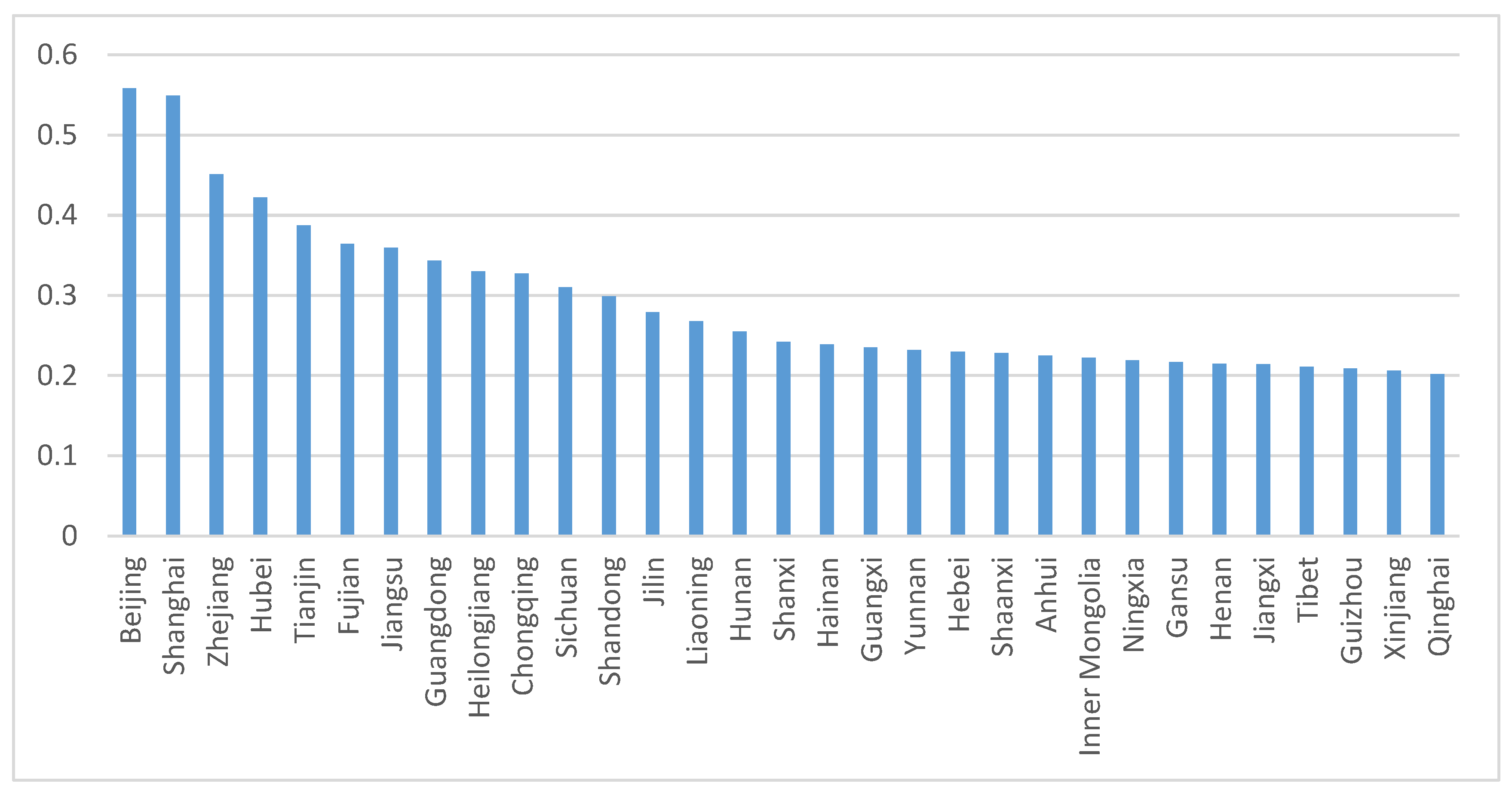
Region	Average Comprehensive Evaluation Index	Region	Average Comprehensive Evaluation Index	Region	Average Comprehensive Evaluation Index	Region	Average Comprehensive Evaluation Index
Beijing	0.558	Heilongjiang	0.330	Hainan	0.239	Gansu	0.217
Shanghai	0.549	Chongqing	0.327	Guangxi	0.235	Henan	0.215
Zhejiang	0.451	Sichuan	0.310	Yunnan	0.232	Jiangxi	0.214
Hubei	0.422	Shandong	0.299	Hebei	0.230	Tibet	0.211
Tianjin	0.387	Jilin	0.279	Shaanxi	0.228	Guizhou	0.209
Fujian	0.364	Liaoning	0.268	Anhui	0.225	Xinjiang	0.206
Jiangsu	0.359	Hunan	0.255	Inner Mongolia	0.222	Qinghai	0.202
Guangdong	0.343	Shanxi	0.242	Ningxia	0.219

.

The average comprehensive evaluation index data of rural finance in China’s provinces, municipalities, and autonomous regions from 2010 to 2019 has been depicted through a histogram in Figure 3. Figure 3 indicates that the average value of the comprehensive evaluation index of rural finance in the study area was mostly between 0.2 and 0.3. Beijing had the highest rural financial average composite index, with a value of 0.558. Since Beijing is the center of China’s economy, politics, and culture, and one of the most developed cities in China’s financial system, rural financial institutions are widely distributed, thereby making the level of rural financial development quite advanced. Shanghai ranked second with an average of 0.549. As China’s financial center and one of the financial centers in Asia, Shanghai’s financial development speed is much faster than that of other regions. Therefore, Shanghai possesses a rapid rural financial development speed and advanced rural financial development level. Guizhou, Xinjiang, and Qinghai had the lowest comprehensive evaluation indices of rural finance, with scores below 0.21. These areas are relatively backward in economic and financial development. Thus, the rural financial development in these areas is relatively backward compared with that in other areas.

4. Research on the Coupling and Coordination Degree of Rural Urbanization and Rural Finance

Coupling coordination degree, a concept derived from physics, refers to the interaction between different systems under their own and external influences [45]. Subsequently, this concept has been introduced into the field of economic research by scholars and used to analyze the interaction degree of two or more systems and the interactive relation between systems [46,47]. This method was used in this study to measure the interaction between rural urbanization and rural finance. Accordingly, this study developed a coupling coordination degree model between rural urbanization and rural finance to analyze the coupling and coordinated development between them.

4.1. Coupling Coordination Degree Model

This study first analyzed the coupling relation between the comprehensive index of rural urbanization (CIRU) and the comprehensive index of rural finance (CIRF). Thereafter, the study analyzed the coupling and coordinated development between rural urbanization and rural finance before finally building the coupling coordination degree model of rural urbanization and rural finance as follows [23,48,49]:

$$C={\left\{\frac{CIRU\times CIRF}{{\left((CIRU+CIRF)/2\right)}^2}\right\}}^{\raisebox{1ex}{$1$}\!\left/ \!\raisebox{-1ex}{$2$}\right.}$$

(8)

In the formula, CIRU and CIRF denote the comprehensive indices of rural urbanization and rural finance, respectively. C refers to the coupling degree between CIRU and CIRF, and the value of C is located in [0, 1]. When C = 1, the coupling degree between rural urbanization and rural finance reaches the maximum, indicating that rural urbanization and rural finance reach a benign resonance coupling with each other. When C = 0, the coupling degree reaches the minimum, indicating that the elements between rural urbanization and rural finance are unrelated. However, although the coupling degree can reflect the interaction degree between rural urbanization and rural finance, it does not adequately reflect the coordination degree between them since the development of each region is dynamic. Therefore, based on the coupling degree model, this study established the coupling coordination degree model, which can effectively reflect the coordinated development between rural urbanization and rural finance. The coupling coordination model is as follows:

$$\{\begin{array}{c}D=\sqrt{C\ast T}\\ T=\alpha \times U_1+\beta \times U_2\end{array}$$

(9)

D indicates the coupling coordination degree of rural urbanization and rural finance, and the value is in [0, 1]. C indicates the coupling degree between urbanization and rural finance. T denotes the coupling coordination index of rural urbanization and rural finance, reflecting the contribution of their overall development level to the coordination degree. The coefficients $\alpha +\beta =1$. Since, in this paper, rural urbanization and rural finance are equally important, it is suggested that $\alpha =\beta =\frac{1}{2}$.

4.2. Classification of the Coupling Degree and Coupling Coordination Degree

Based on the degree of coupling between rural urbanization and rural finance, this study classified the degree of coupling and the degree of coupling coordination between them [24,25,50,51], as presented in

Table 5. Degree of Classification of Coupling Coordination.

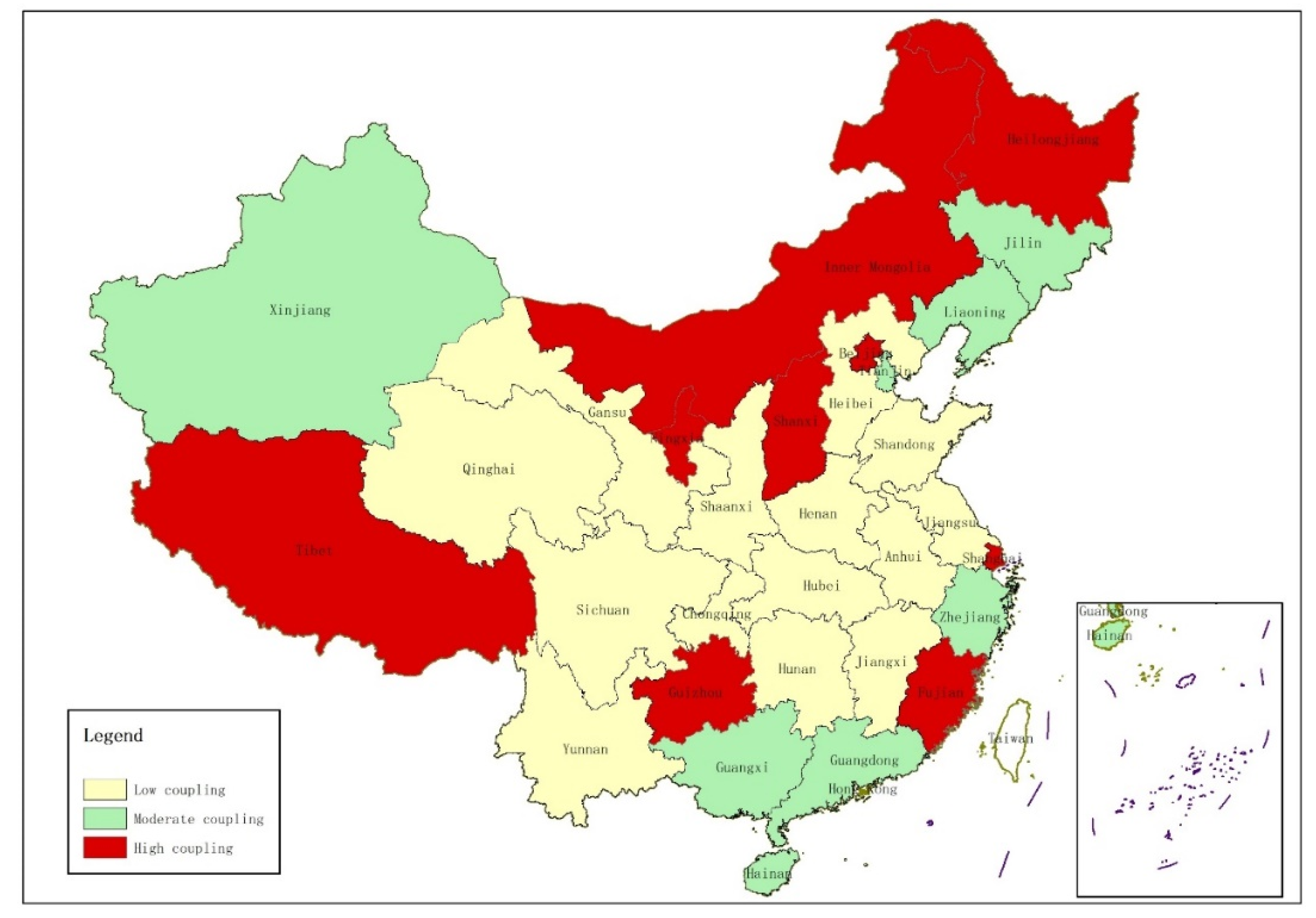
Coupling Value Range	Coupling Degree	Value Range of Coupling Coordination Degree	Coordination Degree
0 < C ≤ 0.4	Low coupling	0 < C ≤ 0.4	Low coordination
0.4 < C ≤ 0.7	Moderate coupling	0.4 < C ≤ 0.7	Moderate coordination
0.7 < C ≤ 1.0	High coupling	0.7 < C ≤ 1.0	High coordination

.

4.3. Measurement of Coupling Degree and Coupling Coordination Degree

4.3.1. Coupling Measurement Results

First, this study calculated the comprehensive indices of rural urbanization and rural finance using the entropy evaluation method by utilizing the comprehensive systems of rural urbanization and rural finance constructed above. Thereafter, the coupling degree model and coupling coordination degree model were employed to calculate the coupling degree and coupling coordination degree of the comprehensive indices of rural urbanization and rural finance from 2010 to 2019. Then, the average value of the coupling degree and coupling coordination degree of China’s provinces, municipalities, and autonomous regions from 2010 to 2019 was taken. According to the degree classification of coupling coordination, this study classified the average coupling degree and coupling coordination degree of China’s provinces, municipalities, and autonomous regions from 2010 to 2019, as presented in

Table 6. Distribution of Coupling Degree.

Coupling Degree	Region	Value of C	Coupling Degree	Region	Value of C	Coupling Degree	Region	Value of C
High coupling degree	Shanghai	0.991	Moderate coupling degree	Xinjiang	0.694	Low coupling degree	Sichuan	0.342
	Beijing	0.990		Jilin	0.676		Hebei	0.325
	Tibet	0.962		Tianjin	0.651		Jiangsu	0.317
	Shanxi	0.926		Guangdong	0.638		Qinghai	0.293
	Inner Mongolia	0.895		Liaoning	0.529		Gansu	0.267
	Fujian	0.885		Zhejiang	0.500		Shaanxi	0.243
	Heilongjiang	0.791		Guangxi	0.472		Yunnan	0.216
	Guizhou	0.726		Hainan	0.466		Chongqing	0.207
	Ningxia	0.714					Hunan	0.157
							Henan	0.152
							Shandong	0.143
							Jiangxi	0.141
							Hubei	0.137
							Anhui	0.126

and Figure 4.

Table 6 and Figure 4 indicate that the average coupling degree of rural urbanization and rural finance was high in nine study areas: Shanghai, Beijing, Tibet, Shanxi, Inner Mongolia, Fujian, Heilongjiang, Guizhou, and Ningxia. The highly coupled areas of rural urbanization and rural finance are either economically developed areas, such as Beijing, Shanghai, and Fujian, or economically backward regions, such as Guizhou, Tibet, and Ningxia. Thus, the development of urbanization and finance closely related to that of economy in this study. In areas with developed rural economies and financial systems, urbanization in rural areas develops faster, and vice versa. Therefore, two extreme situations exist in the highly coupled areas of rural urbanization and rural finance. Eight areas, such as Tianjin, Guangdong, and Zhejiang, were moderately coupled areas. This suggests that the economy of the moderately coupled areas of rural urbanization and rural finance is relatively developed, but a certain gap exists with regard to Beijing and Shanghai. The low-coupling regions included 14 areas, such as Sichuan, Hebei, Henan, and Anhui, and so on. Most of these areas are dominated by agriculture and industry, and rural urbanization and rural financial development are relatively underdeveloped.

4.3.2. Calculation Results of Coupling Coordination Degree

First, the coupling coordination degree of provinces, municipalities, and autonomous regions in China was averaged from 2010 to 2019. Then, according to the ranking of coupling coordination degree, the average coupling coordination degree was classified, as presented in

Table 7. Distribution of Coupling Coordination Degree.

Coordination Degree	Region	Value of D	Coordination Degree	Region	Value of D	Region	Value of D
High coordination degree	Shanghai	0.724	Low coordination degree	Zhejiang	0.321	Qinghai	0.189
	Beijing	0.709		Jilin	0.320	Shaanxi	0.184
Moderate coordination degree	Tibet	0.533		Liaoning	0.308	Gansu	0.175
	Inner Mongolia	0.425		Guizhou	0.294	Chongqing	0.162
	Tianjin	0.426		Jiangsu	0.258	Shandong	0.158
	Fujian	0.422		Hainan	0.256	Yunnan	0.141
Low coordination degree	Shanxi	0.397		Guangxi	0.233	Henan	0.137
	Guangdong	0.378		Hebei	0.207	Jiangxi	0.135
	Heilongjiang	0.364		Anhui	0.204	Hunan	0.132
	Ningxia	0.350		Sichuan	0.202	Hubei	0.127
	Xinjiang	0.332

and Figure 5.

Table 7 and Figure 5 indicate that the average coupling coordination degree of rural urbanization and rural finance in China’s provinces, municipalities, and autonomous regions was relatively low. This suggests that deviation exists in the development of rural urbanization and rural finance in most parts of China, and they do not show synchronous and coordinated paces. Furthermore, only Shanghai and Beijing were highly coordinated, and their average coupling coordination degrees were 0.724 and 0.709, respectively. Four regions, such as Tibet, Tianjin, and Fujian, were moderately coordinated regions. Low coordination areas included 25 regions, such as Shanxi and Guangdong. The coupling coordination degree obviously differed between economically developed and economically backward areas. The more developed the economy, the higher the degree of coupling and coordination between rural urbanization and rural finance; the less developed the economy, the lower the degree of coupling and coordination between rural urbanization and rural finance.

5. An Empirical Analysis of Factors Influencing the Coupling Development of Rural Urbanization and Rural Finance

5.1. Model Building

Coupling and coordination development of rural urbanization and rural finance is affected by many factors, including rural urbanization and rural finance itself, as well as macroeconomic development. This study developed a panel quantile model to empirically analyze the effect of these aforementioned factors on the coupling coordination degree and examine the determinants of the coupling development of rural urbanization and rural finance. This study selected influencing factor indices by Refs. [24,25] and considered indices with larger weights and macroeconomic factors as driving factors of rural finance and rural urbanization. Therefore, this study considered the coupling coordination degree (CCD) of urbanization and rural finance as the dependent variable. For rural urbanization, urban population density (UPD), per capita GDP (PCGDP), per capita disposable income of rural residents (PCDIRR), per capita fiscal expenditure (PCFE), the proportion of educational expenditure to GDP (PEEGDP), and per capita built-up area (PCBA) were chosen as the driving factors. For rural finance, financial development efficiency (FDE), financial development scale (FDSC), and financial development structure (FDST) were selected as the driving factors. The panel data model is built as follows:

$$\begin{gathered} CC{D}_{it}={\beta }_0+{\beta }_{1}UP{D}_{it}+{\beta }_{2}PCGD{P}_{it}+{\beta }_{3}PCDIR{R}_{it}+{\beta }_{4}PCF{E}_{it}+{\beta }_{5}PEEGD{P}_{it} \\ +{\beta }_{6}PCB{A}_{it}+{\beta }_{7}FD{E}_{it}+{\beta }_{8}FDS{C}_{it}+{\beta }_{9}FDS{T}_{it}+{\mu }_{it} \end{gathered}$$

(10)

where, I represents the region, t represents the year, and μ_it represents a random error.

Descriptive statistics were made using the dependent variables, namely the CCD of rural urbanization and rural finance and the driving factors, as presented in

Table 8. Descriptive Statistics.

Variables	Average	Median	Maximum	Minimum	Standard Deviation	Number of Observations
CCD	0.287	0.265	0.763	0.085	0.157	310
UPD	306.503	137.718	3427.409	0.557	609.992	310
PCGDP	42350	36825	107960	639	22835	310
PCDIRR	23418	22638	52859	13188	6443	310
PCFE	10706.83	8646.116	42637.795	854.458	6685.606	310
PEEGDP	5.313	4.592	18.022	2.654	2.381	310
PCBA	68.162	62.676	171.04	39.445	23.008	310
FDE	13414.9	10481.4	54929.9	267.1	10500.8	310
FDSC	8.722	3.585	82.803	1.731	16.54	310
FDST	0.005	0.002	0.049	0.001	0.008	310

.

5.2. Steadiness Test

The panel units of the selected determinants were root tested to avoid the ‘spurious regression’ problem, including the LLC test, Breitung test, and so on [52]. The test results are presented in

Table 9. Root Test Results for Original Sequence Panel Units.

Variables	LLC Test	Breitung Test	IPS Test	ADF-Fisher Test	PP-Fisher Test
UPD	5.305 (1.000)	−2.021 (0.023)	−1.145 (0.126)	6.281 (0.184)	19.709 (0.001)
PCGDP	2.071 (0.908)	−1.462 (0.072)	−2.052 (0.021)	11.330 (0.023)	20.263 (0.000)
PCDIRR	3.359 (0.996)	−1.787 (0.049)	−2.411 (0.059)	13.959 (0.074)	47.847 (0.000)
PCFE	2.272 (0.988)	0.456 (0.675)	−1.601 (0.054)	8.493 (0.071)	25.949 (0.000)
PEEGDP	8.885 (1.000)	0.645 (0.744)	−0.256 (0.393)	3.448 (0.485)	25.343 (0.000)
PCBA	4.573 (1.000)	−0.100 (0.432)	−0.168 (0.431)	3.307 (0.505)	15.369 (0.040)
FDE	4.177 (1.000)	−1.407 (0.098)	−1.684 (0.041)	8.977 (0.063)	26.532 (0.000)
FDSC	3.564 (0.999)	−0.549 (0.296)	−2.210 (0.036)	12.446 (0.014)	21.392 (0.003)
FDST	7.015 (1.000)	−1.180 (0.119)	−0.544 (0.293)	4.074 (0.361)	25.712 (0.000)

Note: The values in () are adjoint probabilities.

.

Table 9 indicates that the original time series of the following determinants were non-steady: urban population density (UPD), per capita GDP (PCGDP), per capita disposable income of rural residents (PCDIRR), per capita financial expenditure (PCFE), the proportion of educational expenditure to GDP (PEEGDP), per capita built-up area (PCBA), financial development efficiency (FDE), financial development scale (FDSC), and financial development structure (FDST). Therefore, a first-order difference was applied on each driving factor, as indicated in

Table 10. First-Order Differential Sequence Panel Unit Root Test Results.

Variables	LLC Test	Breitung Test	IPS Test	ADF-Fisher Test	PP-Fisher Test
UPD	−10.729 (0.000)	−0.876 (0.190)	−10.024 (0.000)	109.234 (0.000)	194.471 (0.000)
PCGDP	−5.429 (0.000)	−2.014 (0.025)	−7.244 (0.000)	76.850 (0.000)	214.820 (0.000)
PCDIRR	−7.129 (0.000)	−1.456 (0.073)	−9.013 (0.000)	78.802 (0.000)	119.619 (0.000)
PCFE	−3.893 (0.000)	−0.810 (0.258)	−9.857 (0.000)	86.134 (0.000)	109.610 (0.000)
PEEGDP	−6.059 (0.000)	−1.638 (0.057)	−12.573 (0.000)	115.354 (0.000)	203.197 (0.000)
PCBA	−5.665 (0.000)	−2.3118 (0.014)	−9.178 (0.000)	80.131 (0.000)	205.054 (0.000)
FDE	−8.468 (0.000)	−2.345 (0.093)	−9.399 (0.000)	81.835 (0.000)	201.094 (0.000)
FDSC	−6.188 (0.000)	−2.125 (0.018)	−9.532 (0.000)	82.190 (0.000)	202.226 (0.000)
FDST	−2.873 (0.002)	−2.542 (0.061)	−8.512 (0.000)	82.236 (0.000)	219.880 (0.000)

Note: The values in () are adjoint probabilities.

. Clearly, all driving factors were statistically significant, so their time series of first-order difference was steady.

5.3. Empirical Analysis Based on Panel Quantile Model

Due to the large gap between rural urbanization and rural financial development in China’s provinces, municipalities, and autonomous regions, especially in the eastern and western regions, the regional differences are more extreme. As a result, this study empirically analyzed the determinants of the coupling development of rural urbanization and rural finance using the panel quantile model to explain the influence of the factors of the coupling coordination degree under different levels of rural urbanization and rural finance.

This study empirically analyzed the quantiles of q value, ranging from (and including) 0.1 to 0.9. The steadiness of the selected model should be first tested. In the primary step, OLS regression of the ordinary panel was carried out for each influencing variable. The regression results are presented in

Table 11. OLS Regression of Normal Panels.

Model 1: OLS Regression of Normal Panels
Constant C	UPD	PCGDP	PCDIRR	PCFE	PEEGDP	PCBA	FDE	FDSC	FDST	R2
−1507.0 *** (72.330)	−0.292 (0.319)	0.032 ** (0.056)	0.022 (0.032)	99.228 *** (13.618)	−1.091 (3.320)	1450.292 *** (934.5)	0.021 (0.042)	−0.034 * (0.014)	0.072 ** (0.024)	0.989

Note: (1) ***, **, and * respectively indicate that they are significant at the levels of 1%, 5%, and 10%. (2) The values in () represent the standard error.

. In the OLS regression of the general panel, the per capita GDP (PCGDP), per capita financial expenditure (PCFE), per capita built-up area (PCBA), financial development scale (FDSC), and financial development structure (FDST) were statistically significant. Therefore, these factors significantly affect the coupling coordination degree of rural urbanization and rural finance. However, the density of urban population (UPD), disposable income per capita of rural residents (PCDIRR), proportion of educational expenditure to GDP (PEEGDP), and efficiency of financial development (FDE) were not statistically significant, implying no significant effect on the coupling coordination degree.

The panel quantile model was used for evaluation, and the results are presented in

Table 12. Panel Quantile Regression.

Model 2: Panel Quantile Regression
Quantile	q = 0.1	q = 0.2	q = 0.3	q = 0.4	q = 0.5	q = 0.6	q = 0.7	q = 0.8	q = 0.9
Constant C	−1502.8 *** (180.299)	−1590.3 *** (190.221)	−1609.6 *** (121.229)	−1704.2 *** (163.940)	−1830.4 *** (144.111)	−1848.0 *** (138.509)	−1898.2 *** (128.628)	−1861.9 *** (130.128)	−1888.9 *** (120.841)
UPD	−5.198 ** (1.335)	−5.224 ** (1.296)	−3.907 ** (1.584)	−3.462 ** (9.897)	−3.123 ** (0.791)	−3.709 ** (0.271)	−2.820 ** (1.436)	−2.236 (2.099)	−2.182 (2.184)
PCGDP	0.0352 ** (0.011)	0.032 ** (0.013)	0.023 ** (0.015)	0.054 ** (0.021)	0.056 ** (0.019)	0.054 ** (0.012)	0.059 ** (0.018)	0.055 ** (0.012)	0.072 ** (0.011)
PCDIRR	−0.085 * (0.038)	−0.085 (0.068)	−0.093 (0.073)	−0.038 (0.087)	0.016 (0.047)	0.011 (0.040)	0.094 (0.043)	0.046 (0.051)	0.019 (0.048)
PCFE	327.188 *** (61.163)	317.195 *** (71.528)	297.526 *** (63.824)	266.323 *** (47.114)	272.801 *** (31.140)	268.387 *** (29.024)	222.122 *** (49.582)	182.901 *** (84.220)	202.227 ** (79.170)
PEEGDP	14.293 ** (4.501)	8.824 * (4.383)	9.126 * (2.179)	−1.549 (6.522)	−0.066 (6.838)	−1.225 (6.218)	−6.097 (7.275)	−5.186 (5.216)	−4.105 (4.166)
PCBA	95544 *** (15023)	111090 *** (14250)	116657 *** (11004)	144944 *** (12937)	147826 *** (15482)	152174 *** (15582)	166458 *** (18272)	169663 *** (19233)	171865 *** (15922)
FDE	−0.039 * (0.0297)	−0.056 * (0.0316)	−0.047 (0.0167)	−0.019 (0.016)	−0.013 (0.025)	−0.015 (0.024)	0.098 (0.034)	0.018 (0.043)	0.021 (0.057)
FDSC	0.038 * (0.096)	−0.044 * (0.019)	−0.025 * (0.028)	−0.023 * (0.005)	−0.010 ** (0.004)	−0.085 ** (0.059)	−0.014 * (0.018)	−0.010 * (0.011)	−0.015 * (0.017)
FDST	0.013 (0.014)	0.040 * (0.011)	0.047 ** (0.019)	0.074 ** (0.024)	0.048 *** (0.012)	0.048 *** (0.013)	0.056 ** (0.013)	0.053 ** (0.016)	0.043 ** (0.013)
Pseudo R2	0.987	0.984	0.983	0.987	0.980	0.981	0.980	0.984	0.986

Note: (1) ***, **, and * respectively indicate that they are significant at the levels of 1%, 5%, and 10%. (2) The values in () represent the standard error.

. The regression results for each significant and non-significant driving factor were highly similar to those for the OLS regression of the normal panel. Therefore, the empirical results of the panel quantile model are steady.

Based on OLS regression results and panel quantile model estimation, the following results can be obtained:

(1)

The regression coefficient of urban population density was negative and significant from (at) q = 0.1 to q = 0.7, but not from (at) q = 0.8 and q = 0.9. This indicates that, compared with the areas with a higher coupling coordination degree, the effects of urban population density (UPD) are more significant in those with a low coupling coordination degree. Moreover, the population density in urban areas negatively affected the coupling coordination degree of rural urbanization and rural finance, and it may have a greater effect where the degree is higher. Although urban population density affected the coupling coordination degree of rural urbanization and rural finance, the effect was related to the coupling coordination degree in the current period. This occurred because urban population density was subordinate to population urbanization. When the coupling coordinated development of rural urbanization and rural finance in an area is low, the increase of urban population density will destroy the original balance and negatively affect the coupling coordination degree of rural urbanization and rural finance. When the coupling coordinated development of rural urbanization and rural finance in a region is relatively high, the influence of urban population density on the coupling coordination degree cannot be clearly reflected. The per capita disposable income of rural residents (PCDIRR) was not significant in Model 1 and Model 2 and negatively correlated with the coupling coordination degree of rural urbanization and rural finance.

(2)

The proportion of educational expenditure to GDP (PEEGDP) was not significant in Model 1. In Model 2, the proportion of educational expenditure to GDP was significant and positively correlated from (at) q = 0.1 to q = 0.3. The major reason is that most areas below 30% of the coupling coordination degree between rural urbanization and rural finance are those with backward educational capabilities, such as Guizhou and Yunnan; thus, increasing the proportion of educational expenditure to GDP will promote the development of rural urbanization in these areas. The increase of educational expenditure indicates that the investment in rural areas in these areas is augmenting, thereby promoting the development of the financial industry. Finally, this process will promote the coupling coordination between rural urbanization and rural finance. However, after the quantile of q = 0.3, the effect of education expenditure on the proportion of GDP was not significant. It can be explained that the educational level is better in areas where the coupling coordination degree of rural urbanization and rural finance is more than 30%. Thus, the increase of education funds cannot significantly affect the coupling coordination degree of rural urbanization and rural finance. From the regression coefficient of the model, the influence of the proportion of education expenditure to GDP on the coupling coordination degree of rural urbanization and rural finance gradually decreased. Areas with a low degree of coupling coordination positively affected the degree of coupling coordination; with its increase, the effect became smaller. For areas with a higher degree of coupling coordination, increasing educational expenditure reduced the degree of coupling coordination. However, on the contrary, financial development efficiency (FDE) exerted the opposite influence, indicating that the effect of financial development efficiency on the coupling coordination degree between rural urbanization and rural finance may increase gradually. In areas with a low degree of coupling coordination, the effect of financial development efficiency was negative; in areas with a high degree of coupling coordination, the effect of financial development efficiency was positive.

(3)

In Model 1 and Model 2, the effect of per capita GDP (PCGDP) was significant, from q = 0.1 to q = 0.9, and positively correlated with the coupling coordination degree of rural urbanization and rural finance. GDP per capita reflects the per capita output value of a region. The increase of GDP per capita will promote the development of urbanization in rural areas. Furthermore, the increase of GDP per capita in rural areas indicates that the economic development in this area is flourishing, thereby developing the rural financial industry. At this time, the development of rural finance and rural urbanization will be more coordinated. Similarly, the effect of per capita fiscal expenditure (PCFE) within the quantiles ranging from q = 0.1 to q = 0.9 was positive, indicating that the coupling coordination development of rural urbanization and rural finance was promoted.

(4)

In Model 1 and Model 2, the per capita built-up area (PCBA) was significant within the quantiles ranging from q = 0.1 to q = 0.9 and positively correlated with the coupling coordination degree of rural urbanization and rural finance. The per capita area of built-up areas reflects the level of urbanization in a region and the regional economic development. If a region has a large built-up area per capita, the urbanization degree of rural areas in the region is high. Higher efficiency of rural urbanization will promote the development of rural economy, subsequently promoting the development of rural finance. Therefore, the increase of built-up area per capita leads to more coordinated rural urbanization and rural finance.

(5)

The regression coefficient of financial development scale (FDSC) was statistically significant. At quantile q = 0.1, the regression coefficient was positive. Within quantiles ranging from q = 0.2 to q = 0.9, the regression coefficient was negative. This indicates that, in areas with a low degree of coupling coordination, the scale of rural financial development significantly positively affected the coupling coordination of rural urbanization and rural finance. However, in areas with a high degree of coupling coordination, the scale of rural financial development significantly negatively correlated with the degree of coupling coordination. The possible reason for this is that, in areas with a low degree of coupling coordination, the growth of rural financial development scale can directly affect the coupling and coordination degree of rural urbanization and rural finance, thereby promoting their coupled development. In areas with a high degree of coupling coordination, the role of rural financial development scale is not obvious, thereby reducing the coupling and coordination of rural urbanization and rural finance.

(6)

The financial development structure (FDST) mainly indicates the allocation structure and resource distribution structure of rural financial funds. In Model 1, the financial development structure was statistically significant. In Model 2, despite its not being significant at quantile of q = 0.1, it was significant within quantiles from q = 0.2 to q = 0.9 and positively correlated with the coupling coordination degree of rural urbanization and rural finance. This indicates that, in the areas where the coupling coordination degree of rural urbanization and rural finance is more than 20%, the optimization of rural financial development structure will make the allocation of funds more reasonable, can significantly promote the development of rural economy, and can promote the coordinated development of rural urbanization. Consequently, the optimization of the financial development structure will promote the coordination between rural urbanization and rural finance.

6. Conclusions and Policy Recommendation

This study selects panel data comprising 31 provinces, municipalities, and autonomous regions in China from 2010 to 2019. First, comprehensive evaluation systems of rural urbanization and rural finance are constructed using the entropy evaluation method, and a comprehensive score is calculated, that is, the comprehensive evaluation index. Second, the coupling model analyzes the comprehensive evaluation index, and the coupling degree and coupling coordination degree of rural urbanization and rural finance are measured. Finally, panel quantile regression is conducted to empirically analyze factors determining the coupling and coordinated development of rural urbanization and rural finance. In this process, the study considers the coupling coordination degree of rural urbanization and rural finance as the dependent variable. The following items are considered as influencing factors to build a panel data model: urban population density (UPD), per capita GDP (PCGDP), per capita disposable income of rural residents (PCDIRR), per capita fiscal expenditure (PCFE), the proportion of educational expenditure to GDP (PEEGDP), per capita built-up area (PCBA), financial development efficiency (FDE), financial development scale (FDSC), and financial development structure (FDST). Consequently, this study draws the following conclusions.

First, the average value of the comprehensive evaluation index of rural urbanization in China’s provinces mostly falls within the range between 0.2 and 0.3. Shanghai has the highest average comprehensive index of urbanization in rural areas, followed by Beijing. By contrast, Gansu, Yunnan, Qinghai, and Guizhou have the lowest indices. The average value of the comprehensive rural financial evaluation index mostly falls between 0.2 and 0.3. The highest index belongs to Beijing, followed by Shanghai. Guizhou, Xinjiang, and Qinghai have the lowest indices.

Second, the coupling model is employed to calculate the coupling degree and coupling coordination degree of the comprehensive evaluation systems of rural urbanization and rural finance. In terms of the average coupling degree of rural urbanization and rural finance, nine provinces achieve a high coupling degree: Shanghai, Beijing, Tibet, Shanxi, Inner Mongolia, Fujian, Heilongjiang, Guizhou, and Ningxia. The areas with a moderate coupling degree include eight provinces, such as Tianjin, Guangdong, and Zhejiang. Areas with a low coupling degree include 14 provinces, such as Sichuan, Hebei, Henan, and Anhui. The research indicates that the average coupling coordination degree of rural urbanization and rural finance is low in most areas. This result indicates a disharmony between the development of rural urbanization and rural finance in most provinces in China, as well as a lack of coordinated development.

Finally, the panel quantile model regression results reveal that, compared with the areas with a higher coupling coordination degree, the effects of urban population density are more significant in those with a low coupling coordination degree. Moreover, the population density in urban areas negatively affected the coupling coordination degree of rural urbanization and rural finance, and it may have a greater effect where the degree is higher. The effect of per capita disposable income of rural residents is not significant and negatively relates to the coupling degree. As the quantile increases, the proportion of education expenditure to GDP presents a decreasing effect on the coupling coordination degree of rural urbanization and rural finance, while the effect of financial development efficiency on the coupling coordination degree is augmenting. Per capita GDP, per capita financial expenditure, and per capita built-up area significantly affect all the quantiles, indicating a positive correlation. This can promote the coupling coordination development of rural urbanization and rural finance. In areas with a low degree of coupling coordination, the scale of financial development significantly positively affects the coupling coordination degree of rural urbanization and rural finance. In areas with a high degree of coupling coordination, the scale of financial development significantly negatively correlates with the coupling coordination degree. A positive correlation exists between the financial development structure and the coupling coordination degree of rural urbanization and rural finance.

Based on the aforementioned conclusions, this study proposes the following recommendations to promote the coordinated coupling development of rural urbanization and rural finance.

First, promoting per capita GDP and increasing per capita fiscal expenditure in rural areas help to promote rural economic development. Rural areas located in economically developed provinces can introduce advanced production technology to improve the per capita output of rural residents, while those located in economically backward provinces can introduce a large number of enterprises to improve the utilization rate of the labor force. Moreover, increasing per capita fiscal expenditure helps to encourage rural residents to consume. Ultimately rural economic development can be promoted to facilitate the coordinated coupling development of rural urbanization and rural finance.

Second, investment in rural infrastructure construction and rural educational expenditure should be increased. Increasing the construction of rural roads, living facilities, and public facilities promotes the spatial urbanization rate in rural areas. Increasing the rural educational expenditure enhances the rate of rural population urbanization and social urbanization by improving the quality of rural residents, and rural finance can become more active through the investment.

Finally, improving the rural financial development scale and optimizing the rural financial development structure are essential. Rural finance can be incorporated into the formal financial market by gradually relaxing the control of rural finance and expanding the rural finance scale. Furthermore, reducing the risk of rural finance is essential through optimizing the rural financial structure and enhancing the competitiveness of rural finance in the overall financial market. In addition, the government should actively improve the relevant rural financial systems to ensure the normal and orderly development of rural financial markets.

References

- Lu, M. From Dispersion to Agglomeration: Theory, Misunderstanding and Reform of Rural Urbanization. Issues Agric. Econ. 2021, 9, 27–35. [Google Scholar]
- Luo, B. Study on Rural Urbanization. Issues Agric. Econ. 2021, 9, 4. [Google Scholar]
- King, R.G.; Levine, R. Finance and Growth—Schumpeter Might Be Right. Q. J. Econ. 1993, 108, 717–737. [Google Scholar] [CrossRef]
- Meyer-Clement, E. Rural urbanization under Xi Jinping: From rapid community building to steady urbanization? China Inf. 2020, 34, 187–207. [Google Scholar] [CrossRef]
- Ahlers, A.L. Weaving the Chinese Dream on the Ground? Local Government Approaches to “New-Typed” Rural Urbanization. J. Chin. Political Sci. 2015, 20, 121–142. [Google Scholar] [CrossRef]
- Ha, T.V.; Tuohy, M.; Irwin, M.; Tuan, P.V. Monitoring and mapping rural urbanization and land use changes using Landsat data in the northeast subtropical region of Vietnam. Egypt. J. Remote Sens. Space Sci. 2020, 23, 11–19. [Google Scholar] [CrossRef]
- Yep, R. Local alliances in rural urbanization: Land transfer in contemporary China. China Inf. 2020, 34, 168–186. [Google Scholar] [CrossRef]
- Mughal, M.A.Z. Rural urbanization, land, and agriculture in Pakistan. Asian Geogr. 2019, 36, 81–91. [Google Scholar] [CrossRef]
- Butler, J.; Wildermuth, G.A.; Thiede, B.C.; Brown, D.L. Population Change and Income Inequality in Rural America. Popul. Res. Policy Rev. 2020, 39, 889–911. [Google Scholar] [CrossRef]
- Labbe, D. Critical reflections on land appropriation and alternative urbanization trajectories in periurban Vietnam. Cities 2016, 53, 150–155. [Google Scholar] [CrossRef]
- Kumar, A.; Sharma, S.; Mahdavi, M. Machine Learning (ML) Technologies for Digital Credit Scoring in Rural Finance: A Literature Review. Risks 2021, 9, 192. [Google Scholar] [CrossRef]
- Blakeslee, D.; Chaurey, R.; Fishman, R.; Malik, S. Land Rezoning and Structural Transformation in Rural India: Evidence from the Industrial Areas Program. World Bank Econ. Rev. 2022, 36, 488–513. [Google Scholar] [CrossRef]
- Abate, G.T.; Rashid, S.; Borzaga, C.; Getnet, K. Rural Finance and Agricultural Technology Adoption in Ethiopia: Does the Institutional Design of Lending Organizations Matter? World Dev. 2016, 84, 235–253. [Google Scholar] [CrossRef] [Green Version]
- Zhou, L.; Feng, H.; Dong, X. From State Predation to Market Extraction: The Political Economy of China’s Rural Finance, 1979–2012. Mod. China 2016, 42, 607–637. [Google Scholar] [CrossRef]
- Qian, M.J.; Huang, Y.S. Political institutions, entrenchments, and the sustainability of economic development—A lesson from rural finance. China Econ. Rev. 2016, 40, 152–178. [Google Scholar] [CrossRef]
- Khanal, A.R.; Omobitan, O. Rural Finance, Capital Constrained Small Farms, and Financial Performance: Findings from a Primary Survey. J. Agric. Appl. Econ. 2020, 52, 288–307. [Google Scholar] [CrossRef] [Green Version]
- Wu, Y.H.; Wu, P.; Ma, W.C. The Inclusive Reform of Rural Finance in Eastern Coastal Areas under the Background of Internet Finance and Its Promotion to Fishery Economy. J. Coast. Res. 2020, 115, 31–34. [Google Scholar] [CrossRef]
- Tang, S.; Zhang, C. Empirical research on the role of rural financial development in rural urbanization. J. Commercial Econ. 2013, 20, 60–62. [Google Scholar]
- Ding, R.; Duan, Y. Construction of the Rural Financial System: The Important Impetus in Accelerating China’s Urbanization. Financ. Econ. 2014, 1, 10–18. [Google Scholar]
- Yan, L.; Yang, W. The role of finance in rural Urbanization development. Agric. Econ. 2015, 8, 114–115. [Google Scholar]
- Yu, J.; Kong, W. A Study on the Change and Reform of the Environment for Rural Finance in China: Under the Background of Rural Urbanization. J. Peking Univ. Philos. Soc. Sci. 2016, 53, 106–112. [Google Scholar]
- Ran, M.; Ran, X. Selection of organizational Forms of rural financial institutions in the process of rural Urbanization. Rural Econ. 2017, 11, 75–78. [Google Scholar]
- Liu, X.; Wang, S. Research on the relationship between urbanization and financial development based on coupling Perspective. Stat. Decis. 2016, 20, 167–170. [Google Scholar]
- Wen, X.; Wang, C.; Xiong, Y.; Xiao, J.; Xie, W. Coupling Coordination Development between New Urbanization and Financial Support in Hunan Province. Econ. Geogr. 2019, 39, 96–105. [Google Scholar]
- Tang, W.; Tang, T. Study on the Coupling Effect Between New Urbanization Development and Financial Support in the Central Provinces’ Cities. China Soft Sci. 2017, 3, 140–151. [Google Scholar]
- Wang, G.; Ye, S. Research on the coordination between economic growth, financial development and urbanization from the perspective of space: A case study of Urban agglomerations in China. Inquiry Econ. Issues 2016, 11, 51–58. [Google Scholar]
- Johnson, K.M.; Lichter, D.T. Metropolitan Reclassification and the Urbanization of Rural America. Demography 2020, 57, 1929–1950. [Google Scholar] [CrossRef]
- Moomaw, R.L.; Shatter, A.M. Urbanization and economic development: A bias toward large cities? J. Urban Econ. 1996, 40, 13–37. [Google Scholar] [CrossRef] [Green Version]
- Kalnay, E.; Cai, M. Impact of urbanization and land-use change on climate. Nature 2003, 423, 528–531. [Google Scholar] [CrossRef]
- Hu, Z.; Chen, H. An empirical analysis of rural financial development, Urbanization and urban-rural income gap. Inquiry Econ. Issues 2013, 6, 63–68. [Google Scholar]
- Chen, S. Local Financial Structure, Government Behavior and Economic Performance in Rural Areas. J. Quant. Tech. Econ. 2009, 26, 81–90+105. [Google Scholar]
- Ren, B.; Yao, B. Empirical Study on Relationship between Farmers’ Property Income and Rural Financial Development in the Process of Urbanization. Mod. Financ. Econ. J. Tianjin Univ. Financ. Econ. 2013, 33, 45–51+61. [Google Scholar]
- Xie, J. The Impact of the Rural Financial Development on the Urban-Rural Income Gap in China: Mechanism Simulation and Empirical Test. Econ. Probl. 2016, 2, 103–110. [Google Scholar]
- Wang, J. Rural Financial Development, Capital Stock Increase, and Rural Economy Growth. J. Quant. Tech. Econ. 2018, 35, 64–81. [Google Scholar]
- Wang, X.; Guan, J. The Income Distribution Effect and Measure of Rural Financial Inclusion in China. China Soft Sci. 2014, 8, 150–161. [Google Scholar]
- Sun, Y.; Zhou, N.; Li, P. Research on the rural residents’ income effect of rural financial development. Stat. Res. 2014, 31, 90–95. [Google Scholar]
- Li, D. The impact of financial development on farmers’ income in China’s prefecture-level cities: A Case study of 17 cities in Shandong Province. Shandong Soc. Sci. 2018, 12, 36–46. [Google Scholar]
- Ding, Z.; Zhang, Y.; Gao, Q. Analysis of rural financial factors influencing rural economic development based on regional economic differences. Chin. Rural Econ. 2014, 3, 4–13+26. [Google Scholar]
- Lin, Y.; Christopher, G.; Xie, Z. Research on the impact of rural financial market competition on the credit risk of rural credit Cooperatives: Based on the data of Fujian county rural credit cooperatives. J. Agrotech. Econ. 2017, 01, 85–97. [Google Scholar]
- Li, H.; Zhang, Q. An empirical analysis of the impact of rural financial development on farmers’ non-agricultural income. Stat. Decis. 2019, 35, 111–114. [Google Scholar]
- Guo, G.; Wang, X. The Rural Financial Supporting to Rural Economic Development in Central Region: Empirical Analysis Based on Panel Date from 2002 to 2011. Syst. Eng. 2012, 30, 86–91. [Google Scholar]
- Jia, L.; Tang, M.; Hu, J. The Measurement and Empirical Analysis on China’s Rural Financial Maturity. J. Nanjing Audit. Univ. 2017, 14, 21–28. [Google Scholar]
- Liu, S.; Zhu, J. The Income Effect of Rural Finance Based on RD-ARDL-SSpace Model. Syst. Eng. 2018, 36, 13–23. [Google Scholar]
- Zhu, J.; Li, R. Mechanism analysis of rural finance influencing green development in western China under the background of rural revitalization: A case study of Guizhou Province. Jiangsu Agric. Sci. 2021, 49, 1–7. [Google Scholar]
- Tang, Z. An integrated approach to evaluating the coupling coordination between tourism and the environment. Tourism Manag. 2015, 46, 11–19. [Google Scholar] [CrossRef]
- Wang, R.; Cheng, J.H.; Zhu, Y.L.; Lu, P.X. Evaluation on the coupling coordination of resources and environment carrying capacity in Chinese mining economic zones. Resour. Policy 2017, 53, 20–25. [Google Scholar] [CrossRef]
- Zhang, Y.J.; Su, Z.G.; Li, G.; Zhuo, Y.F.; Xu, Z.G. Spatial-Temporal Evolution of Sustainable Urbanization Development: A Perspective of the Coupling Coordination Development Based on Population, Industry, and Built-Up Land Spatial Agglomeration. Sustainability 2018, 10, 1766. [Google Scholar] [CrossRef] [Green Version]
- Li, Y.; Li, R.; Jin, H. Nonlinear Effect of Financial Ecology Coupling on New Urbanization: An Empirical Study Based on Double Threshold Panel Data Model. Mod. Financ. Econ. J. Tianjin Univ. Financ. Econ. 2016, 36, 36–44. [Google Scholar]
- Yuan, J.; Wu, Y. Evaluation on the Level and Coupling of Countryside Development in China under the Strategy of Rural Revitalization. J. Agro. For. Econ. Manag. 2018, 17, 218–226. [Google Scholar]
- Geng, Y.Q.; Wei, Z.J.; Zhang, H.; Maimaituerxun, M. Analysis and Prediction of the Coupling Coordination Relationship between Tourism and Air Environment: Yangtze River Economic Zone in China as Example. Discret. Dyn. Nat. Soc. 2020, 30, 27–33. [Google Scholar] [CrossRef]
- Lai, Z.Z.; Ge, D.M.; Xia, H.B.; Yue, Y.L.; Wang, Z.L. Coupling coordination between environment, economy and tourism: A case study of China. PLoS ONE 2020, 15, 13–26. [Google Scholar] [CrossRef] [PubMed] [Green Version]
- Hausman, J.A. Specification Tests in Econometrics. Econometrica 1978, 46, 1251–1271. [Google Scholar] [CrossRef] [Green Version]