Article

Spatio-Temporal Evolution of Land Use Transition in the Background of Carbon Emission Trading Scheme Implementation: An Economic–Environmental Perspective

1
Mingshi Investment Management, Shanghai 200120, China
2
Department of Investment, School of Finance and Economics, Jimei University, Xiamen 361023, China
*
Author to whom correspondence should be addressed.
Land 2022, 11(3), 440; https://doi.org/10.3390/land11030440
Submission received: 10 February 2022 / Revised: 15 March 2022 / Accepted: 17 March 2022 / Published: 18 March 2022
(This article belongs to the Special Issue Socioeconomic Evaluation of Climate Change Impacts on Land Ecosystems)

Abstract

:
In the political context of “carbon peaking” and “carbon neutrality” proposed by the Chinese government, this paper investigates the spatio-temporal evolution of land use transition in China after the implementation of the carbon emission trading scheme (CETS). Based on the analysis of the spatio-temporal evolution, we discuss the spatial spillover of the policy effects. With the help of China’s CETS policy, this study explores the above issues with the main observation samples of the six provincial pilots included in CETS. Using the entropy weighting method, the indicator construction method, and local Moran’s I test, this paper takes 30 provincial areas in China from 2010 to 2017 as the full sample, and draws the following conclusions: (1) both the economic and environmental effects generated by CETS can optimize land use transition in the pilot areas, but the effective time points of the two are different; (2) the time for land use transition to be optimized by the two effects of CETS is different, among which the economic effect takes effect faster than the environmental effect; and (3) there is spatial spillover of the optimization effect of CETS on land use transition, but the specific effect depends on the industrial structure and development plan of the pilot areas.

1. Introduction

Global climate change is increasingly testing human activities, and more and more countries and regions are putting forward the vision of a “carbon-free future”. In recent years, China has been plagued by environmental problems such as haze pollution, and domestic environmental problems are becoming more and more intense. Environmental pollution has already had a negative impact on China’s economic development [1] and the health of its inhabitants [2,3]. On the other hand, China’s energy structure is dominated by fossil fuels. According to relevant statistics from the Wind database, the share of coal, oil, and natural gas reached 85% in 2019, and the large amount of fossil fuel use has caused a continuous increase in carbon emissions. In 2019, the share of carbon emissions from fossil fuels reached 92%. With China’s declining fossil energy reserves and rising energy costs [4], as well as increased uncertainty over imported energy due to trade conflicts [5], it has become imperative to save energy and reduce emissions. Large amounts of carbon emissions are also causing climate change problems in China [4,6], and the average surface temperature has gradually increased from 7.14 °C in 1990 to 10.17 °C in 2019, with the warming phenomenon becoming more pronounced. Against this background, the Chinese government has been paying long-term attention to greenhouse gas limitations and has enacted a series of measures, and in 2020, it proposed a dual carbon strategy of “carbon peaking” and “carbon neutrality” (CO2 emissions strive to reach a peak by 2030 and strive to achieve carbon neutrality by 2060) [7]. One of the more successful and landmark policies of the period is the carbon emission trading scheme (CETS) [8]. The trading of carbon emission rights is one of the most efficient and promising tools for carbon regulation [9]. China began planning for the implementation of a carbon emission trading scheme as early as October 2011. Between 2013 and 2014, Shenzhen, Shanghai, Beijing, Tianjin, Guangdong, Hubei, and Chongqing were opened as pilot provinces for the carbon emission trading scheme (CETS). The CETS was first proposed by the State Council of the People’s Republic of China in 2011 as part of the Twelfth Five-Year Plan. The primary objective of the CETS is to promote the development of an economic development model with low greenhouse gas emissions. CETS covers seven pilot provinces and cities, mainly covering the eight highly polluting industries of petrochemical, chemical engineering, building, iron and steel, nonferrous metal, paper making, electric power, and air transportation, involving at least 2000 physical enterprises [10]. Using carbon emissions as a benchmark, the growth rate of China’s total carbon emissions has slowed down significantly up to 2017 (Figure 1), and the CETS can be considered successful to some extent [11].
Accompanying the context of China’s aim to limit greenhouse gases is the long-standing land use problem that the country faces. Over the past decades, China’s economic privatization reforms have significantly changed the use of land in China [11]. However, similar to other parts of the world, the urbanization of China has been accompanied by the expansion of urban land areas [12,13] and a proliferation of urban populations. This has been accompanied by serious environmental pollution problems [14] and a gradual decline in land use efficiency [15]. At the same time, with the reduction of newly available land in cities, the allocation of land for various uses is becoming increasingly intense [16], and land use and redistribution are in urgent need of adjustment. On the other hand, along with the improvement of the quality of life of the population, fixed land area is required to be able to produce more economic benefits. Studies have been carried out on the sustainability of land use [17], the economic development of suburban land [18], and the economic benefits of agriculture [19]. At the same time, the contradiction between the economic development and environmental protection faced by developing countries [6] makes it necessary to discuss the two in an organic way.
Land use transition was originally proposed by Grainger [20] and refers mainly to long-term and trending changes in land use patterns within a region [21,22,23]. Among these, land use patterns record the characteristics of socioeconomic development in the region [24,25]. Traditional studies of land use transition have focused on specific land types, such as rural residential land [26] and industrial land [27]. The emergence of the Global Land Project (GLP) has focused international research on environmental change on water systems, carbon, food, and land. As an important part of the GLP, land use transition has received much attention from researchers on how to optimize land use, how to improve the efficiency of resource use, how to adjust the appropriate industrial structure, and how to promote the process of sustainable development [28,29]. At this time, the definition of land use transition has been expanding. In the context of economics, land use transition can refer to the change in land use patterns over time, corresponding to the transition of economic and social development stages. With economic improvement and social development, land use pattern conflicts at the regional level gradually weaken [30], which effectively reflects changes in the natural environment, as well as the process of socio-economic development [31]. Since then, researchers have focused more on the eco-environmental effects [32,33] and driving mechanisms [34] of land use transition.
Van et al. found that an important policy would significantly change the land use transition of a region [35]. The CETS is not only an important attempt to achieve China’s ‘double carbon goal’, but also an environmental regulatory policy tool with both economic [36] and ecological effects [37]. The former changes the regional industrial structure [38], labour supply and demand [39], whereas the latter affects the regional emissions [40], energy use efficiency [41], etc. Therefore, this paper argues that before and after the implementation of CETS, there will be significant changes in the economic and environmental levels in land use transition in its pilot areas. Research discussing the relationship between the environment and land use transition is not uncommon. Froese and Schilling, for example, discuss the relationship between environmental change, land use, and regional conflicts [42]. There are also studies discussing the impact of greenhouse gas emissions on the transformation of arable land [43], the impact of environmental change on urban land use transition [16,33,44], the impact of changes in the hydrological environment on land use [45], and even a strong interaction between environmental change and land use [46], among others. Since CETS is a good exogenous policy shock, most studies prefer to investigate it through double difference-in-difference (DID) estimation methods [47], mainly discussing its policy rationality or economic consequences [11,48]. However, studies exploring the impact of CETS on land use transition are not sufficient. For example, Tang et al. (2022) discussed the impact of CETS on land use transition in terms of the economic, environmental, and Porter effects of CETS using DID estimation [11]. However, their focus is on the causal argument between CETS and land use transition, which fails to reflect the spatio-temporal evolutionary land use patterns under the influence of CETS, and there is still room for further discussion on the spillover effects of CETS. For example, Xia et al. (2021) investigated the mitigation effects of CETS using the DID estimation method, but did not consider the impact of the economic effects generated by CETS, and again did not analyze the spatio-temporal evolution pattern and its possible spillover effects [49]. Arguably, these studies that look at outcomes and ignore spatio-temporal changes in land use transition are clearly inadequate [50,51]. In this strand of the CETS literature on the economic and environmental consequences of land use transition, there should be studies that take a comprehensive look at the dynamic framework over a certain length of time. Based on the above, this paper makes the first type of hypothesis.
Hypothesis 1a (H1a)
CETS optimizes land use transition in the pilot area in terms of the economic effect dimension.
Hypothesis 2a (H2a)
CETS optimizes land use transition in the pilot area in terms of the environmental effect dimension.
Given that innovation takes time to develop [52], and that changes in a company’s business strategy are difficult to make in the short term, it is possible to implement measures such as production reductions more smoothly. This is combined with the finding that the economic effects of CETS work faster than the environmental effects [39]. This paper suggests that the economic and environmental dimensions of CETS have different effects on land use transition optimization. Based on the above, this paper makes the second type of hypothesis.
Hypothesis 1b (H1b)
This optimization effect from the economic effect dimension on land use transition takes effect immediately.
Hypothesis 2b (H2b)
This optimization of land use transition in terms of environmental effects takes effect with a lag.
Tobler once said: “Everything is related to everything else, but near things are more related than distant things” [53]. Although the CETS only acted on the pilot areas, the responses of the pilot areas will likely affect their surrounding areas. For example, a study by Du et al. concluded that CETS had a negative spillover effect on innovation development in neighboring regions [54], whereas a study by Tang et al. found that CETS had a dampening effect on economic development in neighboring regions, but was able to promote improvements in their environmental pollution [11]. This paper argues that the differences in the economic and environmental dimensions of the CETS spillover effects may be due to the current conflict between the economy and the environment in China. Specifically, the pilot companies need to launch innovative activities in order to cope with the CETS, thus creating a siphoning effect that causes capital from neighboring regions to concentrate there, thus inhibiting the economic development of neighboring regions. On the other hand, given the trend of green development, neighboring regions, although not strictly required by the CETS, may still prepare in advance for possible future emission restrictions. The neighboring provinces of the pilot areas, on the other hand, are more likely to learn from the pilot areas, and thus reduce their own pollution emissions, as they have closer economic and political exchanges with the pilot areas. Therefore, this paper makes a third type of hypothesis.
Hypothesis 1c (H1c)
There is a negative spillover effect of this optimization of land use transition in terms of economic effects.
Hypothesis 2c (H2c)
There is a positive spillover effect of this optimization effect on land use transition from the environmental effect dimension.
The possible marginal contributions of this paper are as follows. (1) The current literature on the impact of CETS on land use transition is scarce, and most of them adopt the DID estimation method to determine the causal relationship between them, but pay less attention to their spatio-temporal evolution patterns and spatial spillover phenomena. This study enriches these contents. (2) This paper combines the entropy method, the indicator construction method, and a Moran scatterplot to reflect the spatio-temporal evolution patterns and spillover effects of land use transition more effectively and accurately.
The remaining sections of this paper are as follows. Section 2 introduces the sample areas, research ideas, details of the evaluation system of land use transition, data sources, and applied methods. Section 3 presents the results of the entropy method, and analyzes the spatio-temporal evolution patterns, and spillover effects of land use transition under the influence of CETS. The results obtained in the previous section are discussed in detail in Section 4, and a series of policy implications are obtained for the “double reduction” of carbon emissions in China.

2. Methodology

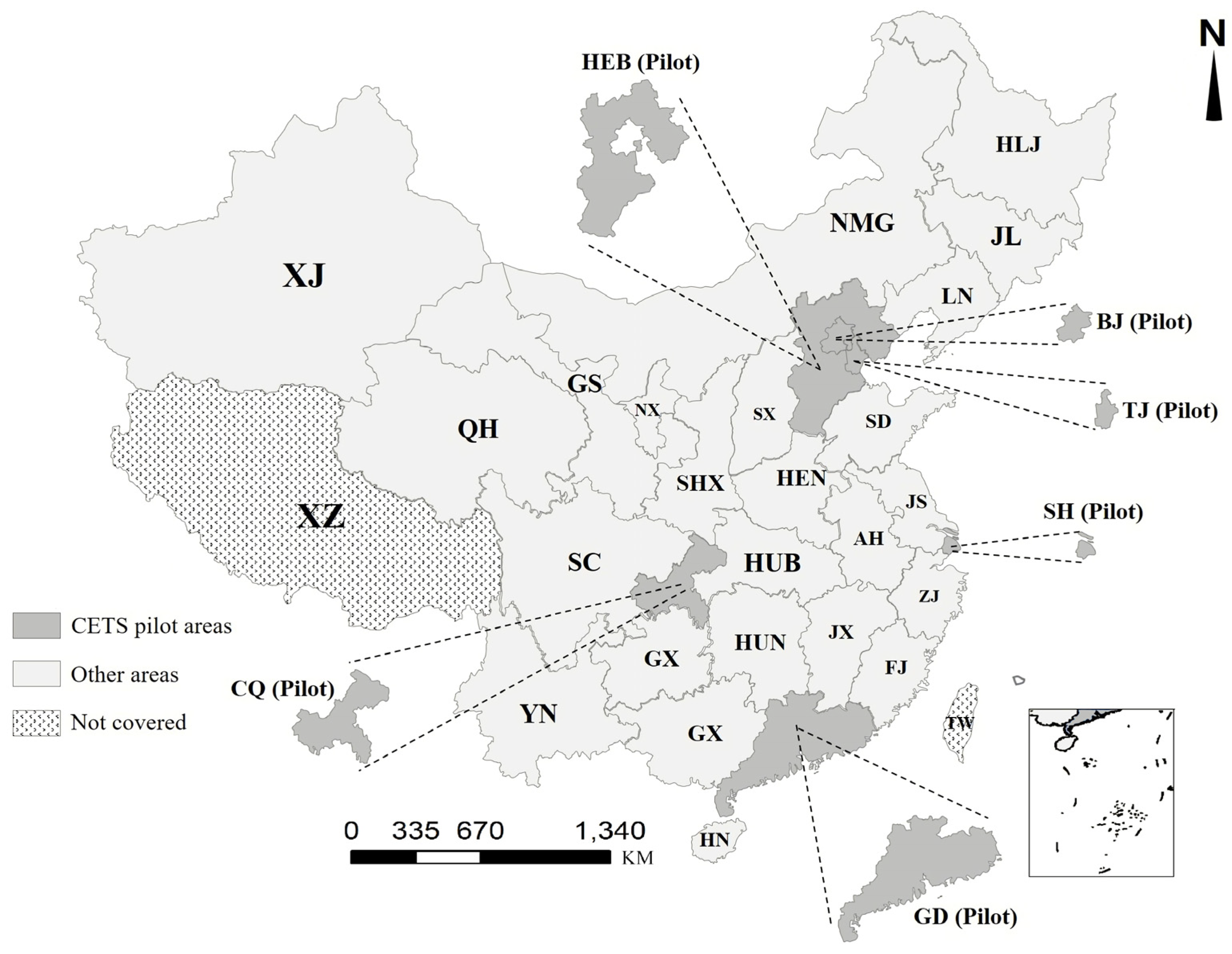
2.1. Introduction of CETS Pilot Regions
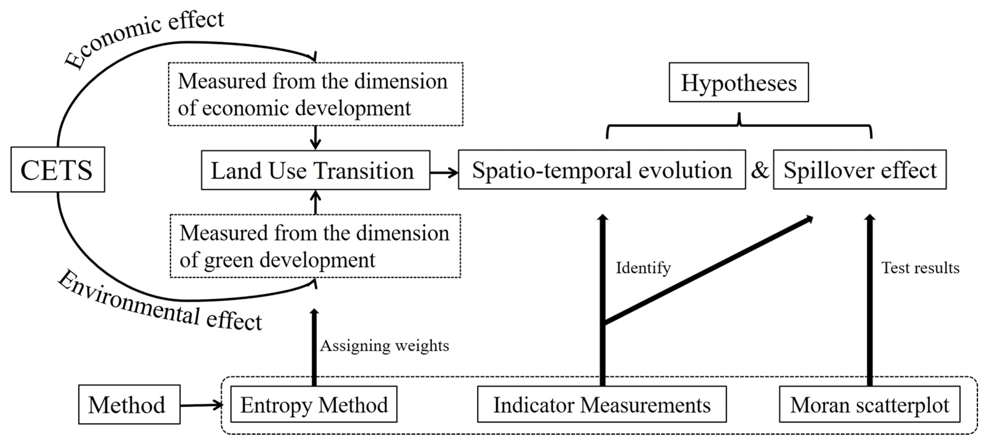
This study focuses on the six pilot provincial regions mentioned in CETS, namely Beijing, Tianjin, Shanghai, Chongqing, Hubei, and Guangdong. These six regions are briefly described in the following section. Figure 2 shows the distribution of these six regions in China.
Beijing is located in northern China (115.7°–117.4° E, 39.4°–41.6° N) and is bordered by Tianjin and Hebei. As of 2020, Beijing has a total area of 16,410.54 km2, a resident population of about 21,893,000, and a GDP of 361,026,000 RMB, ranking 13th in the country (in terms of 31 provincial units, same as below). As of 2017, Beijing’s highest carbon emissions were 90.9 Mt (at 2010), and its carbon emissions have significantly decreased and stabilized since 2013.
Tianjin is located in northern China (116°43′–118°04′ E, 38°34′–40°15′ N), bordering Beijing and Hebei Province. As of 2020, Tianjin has a total area of 11,966.45 km2, a resident population of about 13,866,000, and a GDP of RMB 140,837,300, ranking 23rd in the country. As of 2017, Tianjin’s highest carbon emissions were 150.0 Mt (at 2017), and its carbon emissions are still increasing, but the growth rate is gradually slowing down.
Shanghai is located in eastern China (120°52′–122°12′ E, 30°40′–31°53′ N) and is bordered by Jiangsu and Zhejiang provinces. As of 2020, Shanghai has a total area of 6340.5 km2, a resident population of about 24,870,900 people, and a GDP of 387,006,000 RMB, ranking 10th in the country. As of 2017, Shanghai’s highest carbon emission is 230.7 Mt (at 2010), and its carbon emission trend is the same as that of Beijing.
Chongqing is located in western China (105°11′–110°11′ E, 28°10′–32°13′ N) and is bordered by Hubei and Hunan provinces, Guizhou, Sichuan, and Shaanxi. As of 2020, Chongqing has a total area of 82,402 km2, a resident population of about 32,054,200, and a GDP of 25,002,000 RMB, ranking 17th in the country. As of 2017, Chongqing has the highest carbon emission, at 153.8 Mt (at 2017), but its carbon emissions have generally remained stable and have shown signs of decline since 2010.
Hubei Province is located in central China (108°21′–116°07′ E, 29°01′–33°6′ N), bordering Anhui Province, Chongqing Municipality, Shaanxi Province, Jiangxi Province, Hunan Province, and Henan Province. As of 2020, Hubei Province has a total area of 185,900 km2, a resident population of about 57.75 million, and a GDP of 434,435,000 RMB, ranking 8th in the country. As of 2017, Hubei Province’s highest carbon emission was 338.60 Mt (at 2014), and its carbon emissions have shown a decreasing trend since 2014.
Guangdong Province is located at the southernmost point of mainland China (109°39′–117°19′ E, 20°13′–25°31′ N) and is bordered by Guangxi Province, Hunan Province, Jiangxi Province, Fujian Province, and Hainan Province. Among them, Hainan Province is across the sea. As of 2020, Guangdong Province has a total area of 179,725 km2, a resident population of about 126,012,500, and a GDP of 1,107,609,000 RMB, ranking 1st in the country. As of 2017, the highest carbon emission in Guangdong Province is 521.74 million tons (in 2016), and remains stable year-round.

2.2. Study Strategy

This study aims to investigate the spatio-temporal evolutionary trends of land use transition in economic and environmental dimensions under the influence of CETS. First, we construct an indicator evaluation system for land use transition and measure the land use transition indicators using the entropy method. Secondly, we construct Evolution indicators to identify the spatio-temporal evolution trends of land use transition in different periods and map the Evolution data to understand the possible spillover effects. Meanwhile, a Moran scatterplot is used to further examine and analyze these spillover effects. Finally, the above results are analyzed and discussed to determine the validity of the hypotheses proposed in the study. Figure 3 shows the above process.

2.3. Indicators and Data

2.3.1. Evaluation System of Land Use Transition

According to the previous section, CETS has economic and environmental effects that will affect the land use transition of a region. Therefore, this study constructs the evaluation system of land use transition indicators from the economic dimension and the green development dimension, respectively. The entropy method is used to assign weights to these indicators, and its assignment steps will be executed by Matlab R2016a software. Table 1 summarizes the situation of the land use transition indicator system and the descriptive statistics of each indicator. The data in Table 1 are for 30 provincial regions in China (except Tibet, Hong Kong, Macao, and Taiwan) from 2010–2017.
Under the influence of the economic effect of CETS, the pilot enterprises, especially the highly polluting enterprises, mainly face two choices. One is to reduce or stop production to avoid the “punishment” of exceeding the carbon emission limit. This will also hinder the economic development of the region, thus reducing the economic benefits of land use transition. The second is to implement an innovative transformation. Companies can use this to increase the additional value of their products or services to cover the cost of emissions, or reduce the cost of emissions by innovating pollution control to reduce the amount of emissions produced per unit of product. This will improve the quality of the region’s economy, and thus improve the quality of land use. Based on the above brief analysis, we will measure the economic dimension of land use transition in terms of both economic growth rate and the quality of economic development.
In terms of economic growth, two secondary indicators are selected as components of this study. GDP is an excellent indicator of the level of the economy. Similarly, GDP growth rate is an excellent indicator of the economic growth rate. Considering the large influence of population size on GDP [55], this paper also uses GDP growth rate per capita to exclude this influence.
In terms of economic quality, this study selects three secondary indicators as the components. One is the proportion of the added value of tertiary industries. The improvement of economic quality in a region should be accompanied by the optimization of the industrial structure, which usually refers to the decrease in the proportion of the output value of primary and secondary industries and the increase in the proportion of tertiary industries in China [55,56]. The second is the share of science and technology expenditure. This indicator refers to the proportion of science and technology expenditure in the local government’s fiscal expenditure, which reflects the degree of importance that local governments attach to the construction of innovation development in their regions. Innovation is the driving force of China’s high-quality economic development, the key to harmonizing environmental and economic development [57], and the cornerstone for achieving sustainable development [58,59]. At the same time, the R&D investment of the local government will also drive the innovation behavior of enterprises [60] The third is the full-time equivalent of R&D personnel, which reflects the level of effort of R&D personnel. The output of innovation results requires a large amount of human capital, in which the degree of effort of R&D personnel plays a key role. It can be said that abundant R&D human resources are the key to innovation-driven transformation and high-quality economic development in the region, and are the basis for achieving green development. Its change directly affects the evolution of local land use transition.
Under the influence of the environmental effect of CETS, the pilot enterprises will force themselves to match the policy emission limit standard due to production reduction, shutdown, leaving the polluting industry and strengthening pollution treatment. This situation is reflected in the environmental dimension in the reduction of various types of pollution emissions, thus promoting local green development building. On the other hand, the pilot enterprises, in the process of innovation transformation, will try to increase the unit energy production of their products (China is currently dominated by coal energy consumption, so energy consumption will increase pollution emissions). At the same time, government officials will increase the intensity of investment in pollution control based on the local environmental quality and performance assessment. These methods will help local enterprises and governments to control pollution emissions, which is an important component of green development. Based on the above brief analysis, we will measure the land use transition of the green development dimension in terms of both pollution emission and pollution control.
In terms of pollution emission intensity, four secondary indicators are selected as components in this study. The former three indicators are industrial waste gas, industrial wastewater, and industrial soot, which are the most important pollutants in production, and can effectively reflect the pollution emission from the production activities of enterprises. The fourth one is carbon dioxide emission, which is a pollutant directly controlled by CETS, and will undoubtedly be significantly influenced. In order to avoid the influence of area size on pollutant emissions, this paper divides the emissions of all the above four pollutant emissions by the land area. In addition, since the direction of the above indicators is negative, they need to be transformed into positive indicators before they can be applied to the entropy method. Therefore, we will actually use their inverse values in the weighting process.
In terms of governance initiatives, two secondary indicators are selected as components in this study. One is industrial output efficiency, and the other is the share of investment in pollution control. The former is the ratio of the industrial output’s added value to industrial energy consumption, which reflects the efficiency of energy use by industrial enterprises in the region. The higher the value, the higher the economic return per unit of energy. This helps the region to move towards the right side of the environmental Kuznets curve (EKC) [61], which is important for building a model of green development. The latter is the ratio of pollution control investment to GDP, reflecting the importance that local governments attach to local pollution control. Local governments in China have strong market influence [62]. The degree of importance local governments attach to pollution control determines the intensity of their environmental regulation policies, which can significantly influence firms’ decisions [63,64]. Therefore, the local government’s attention to pollution control will become an essential part of the construction of local green development.

2.3.2. Data Source

The sample of this study comprises 30 provincial-level regions in China, and the sample interval is 2010–2017. This is because 2013 or 2014 are the implementation points of the CETS policy, and the carbon emission data are only updated up to 2017. Therefore, in order to balance the interval before and after the policy point in order to construct the Evolution indicator more effectively, the initial point of the policy is set in 2010 in this paper. On the other hand, since 2010, the Chinese government has paid much more attention to environmental management and promoting green, healthy, and sustainable development than before. Therefore, using 2010 as the starting point can better control the bias due to the context of the era.
The raw data for this study were obtained from the China Statistical Yearbook and the China Research Database Service Platform (CNRDS). Additionally, the raw data for carbon emissions come from the study results of Shan et al., and the China Emission Accounts and Datasets (CEADs) [65,66]. There are some missing data in the study, which are filled by the moving average method in this paper.

2.4. Method

2.4.1. Entropy Method

The entropy method determines the size of the weights based on the degree of variation of the variables between samples. The greater the degree of variation, the greater the weight value. Therefore, the entropy method not only has the function of down-dimensioning, but also has the feature of objective weighting. Therefore, it is also possible to derive the trend of variation in the degree of variation of the factor indicators based on the trend of their weights over the years. The common calculation steps of the entropy method are as follows.
Step 1. Standardize the variables. xi,b,t is the original matrix, i is the cross-sectional ordinal number. In this paper, i is the order number of 30 provinces and cities (0 < i ≤ n), t is the time ordinal number (2010 ≤ t ≤ 2017), and b is the secondary indicator ordinal number (0 < bB). Xi,b,t is for the standardized matrix.
X i . , b , t = x i , b , t min | x i , b , t | max | x i , b , t | min | x i , b , t | ,
Step 2. Calculate the information entropy (Ib,t). Ib,t is constructed by calculating the specific gravity variable (Mi,b,t) from the normalization matrix (Xi,b,t) instead. Where n is the total number of sample cross-sections, and in this paper, n = 30.
I b , t = ln ( n ) 1 i = 1 n ( M i . , b , t ) ln ( M i . , b , t ) M i . , b , t = X i . , b , t i = 1 n X i . , b , t ,
Step 3. Calculate the weight matrix (Weightb,t) according to Equation (3), where K is the total count of secondary indicators.
W e i g h t b , t = 1 I b , t K I b , t .
Step 4. Calculate the value of land use transition (LUTi,t) composite index demanded by this paper. According to Equation (4), the value of land use transition can be measured for area i in period t.
L U T i , t = b = 1 B X i , b , t * W e i g h t b , t .

2.4.2. Analysis Method

This study analyzes the spatio-temporal evolution of land use transition in the economic effect dimension and environmental effect dimension with the help of the Evolution index and a Moran scatterplot. The former can compare the numerical trends of land use transition (LUT) indicators at different periods and reveal their spatial distribution patterns and spillover effects through data mapping. The latter can test the former’s conclusion about the spillover effect and further derive information about the intensity of the spillover effect.
First, the indicator measurement method used in this study is introduced. The purpose of this method is to quantify the extent of changes in LU at different time points. Therefore, we constructed Equation (5).
E v o l u t i o n p r e = L U T i n L U T p r e E v o l u t i o n a f t e r = L U T a f t e r L U T i n
in which Evolution measures the degree of change in LU for both stages. It is worth mentioning that, in order to more effectively assess the impact of the CETS policy on land use transition, we need to obtain an average estimate as much as possible. Moreover, because the CETS policy could have been initiated in 2013 [67] or 2014 [68], this study divides the sample interval into three time periods, i.e., before 2013–2014, 2013–2014, and after 2013–2014. The three represent the time periods before, during, and after the implementation of CETS, which are denoted by the subscripts “pre”, “in”, and “after”, respectively. Thus, Evolutionpre reflects the difference between the CETS implementation process and the pre-implementation process, referred to as the “first stage”, whereas Evolutionafter reflects the difference between the CETS implementation process and the post-implementation process, referred to as the “second stage”. The calculation process of LUpre, LUin and LUafter is shown in Equation (6).
{ L U T p r e = t 2012 L U T i / ( 2012 t + 1 ) ,     i f   t 2012 L U T i n       = ( L U T 2013 + L U T 2014 ) / 2                                     L U T a f t e r = t N L U T t / ( N i + 1 ) ,     i f   t 2015         ,
where t is the year, and N is the sample deadline year.
Next, the Moran scatterplot is introduced. The Moran scatterplot is a method for estimating the local spatial autocorrelation of variables. It can judge the spatial autocorrelation characteristics of each sample if two samples belong to the first quadrant of cartesian coordinates, if they belong to high-value and high-value (H-H) agglomeration, and if there is a positive spillover effect. If two samples belong to low-value and low-value (L-L) agglomeration, they are considered to belong to the third quadrant. Although the statistic is negative at this point, there is still a positive spillover effect between the two areas with negative values. Similarly, the second quadrant is the L-H agglomeration, and the fourth quadrant is the H-L agglomeration, both of which produce negative spillover effects. It is worth mentioning that we can determine the strength of the spillover effect by the difference between the absolute value of the x-coordinate value and the absolute value of the y-coordinate value of the sample statistics in the Moran scatterplot. The greater the absolute value of the y-coordinate value is compared to the x-coordinate value, the stronger the spillover effect. Conversely, when the spillover effect is weaker, Equation (7) describes how to calculate the x and y coordinate values in the Moran scatterplot.
X i , t = Z i , t = E v o l u t i o n i , t E v o l u t i o n t ¯ Y i , t = j i n W i j Z j , t i n   w h i c h ,   Z j , t = E v o l u t i o n j , t E v o l u t i o n t ¯
where both i and j are the serial numbers of the regions. X’i,t denotes the corresponding x-value of the Evolution indicator in the Moran scatterplot for region i in year t. Y’i,t denotes the corresponding y-value. Wij denotes the spatial weight matrix.
The meaning of each symbol is the same as above. In addition, when IL > 0, there are H-H or L-L agglomeration characteristics in adjacent areas; when IL < 0, there are L-H or H-L agglomeration characteristics in adjacent areas; when IL = 0, there are no local agglomeration characteristics in adjacent areas.

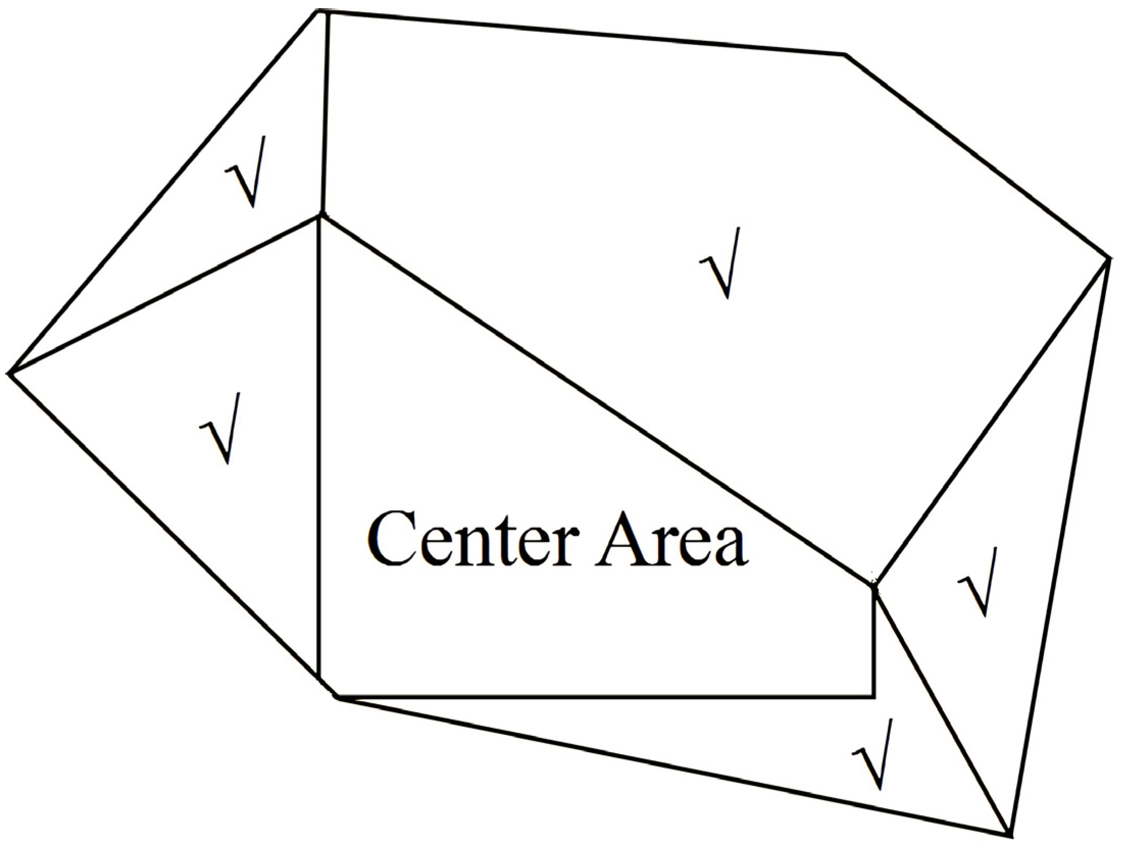
2.4.3. Design of the Spatial Weight Matrix

Tobler’s First Law of Geography pointed out that “everything is related to everything else, but near things are more related to each other” [53]. This implies that we cannot ignore the importance of spatial geographic information. The spatial weight matrix is precisely the tool to quantify spatial geographic information, which is the basis of spatial econometrics. In this study, the first-order contiguity matrix is used for the local spatial autocorrelation test to analyze the clustering of Evolution indicators in the provincial regions of China. In this paper, the first-order contiguity matrix is constructed based on the scheme of queen contiguity (Equation (8)). That is, if there is a common fixed point or boundary between two regions (Figure 4 is the diagram), they are considered to be adjacent; conversely, they are not adjacent. This implies that the scope of the spillover effect emphasized by the first-order contiguity matrix is limited [57].
W i j = { 1 ,   i   a n d   j   a r e   q u e e n   c o n t i g u i t y ,   a n d   i j 0 ,   o t h e r w i s e                                                                             .

3. Results

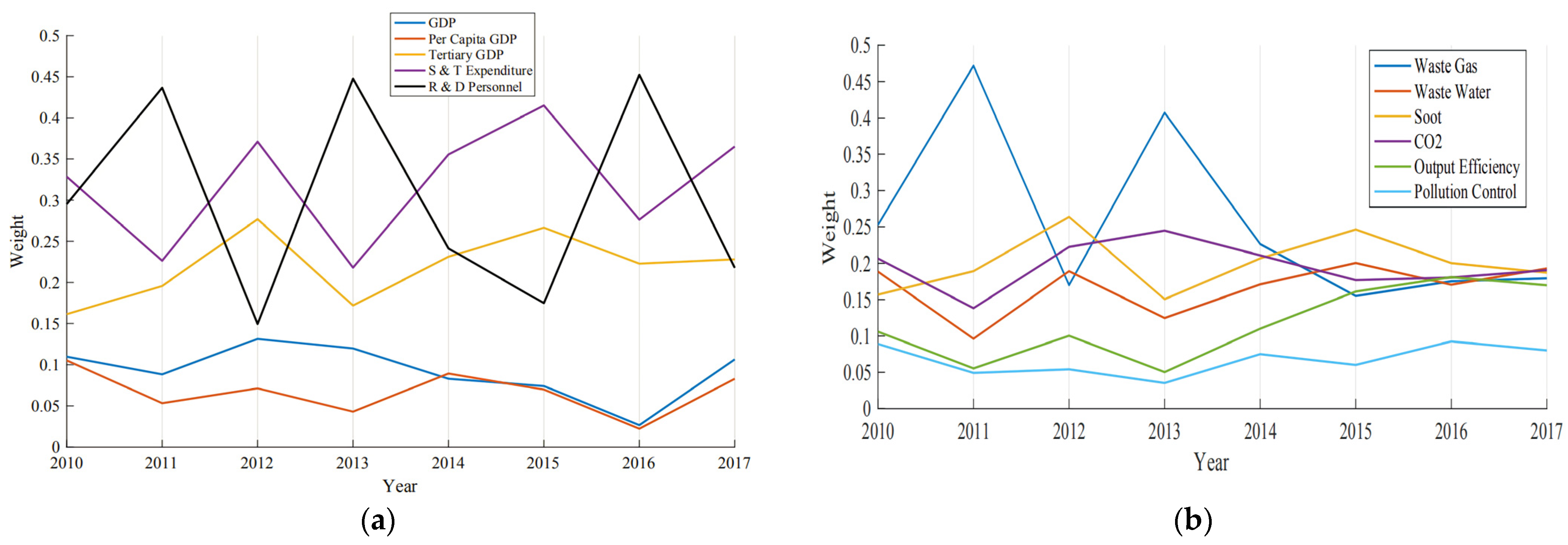
3.1. Results of the Entropy Method

With the help of the Matlab R2016a software, this study measured the score values of land use transition in the economic and green development dimensions separately using the entropy method. Figure 5 shows the trend of weight changes of the secondary indicators (Table 1 for details) that consist of these two land use transition indicators over the period 2010–2017, where Figure 5a shows the economic dimension and Figure 5b shows the green development dimension. The entropy method not only helps this study to quantify the land use transition indicators more objectively, but also enables additional information to be obtained. Based on the trend of weight changes of the secondary indicators, we can determine which secondary indicators are more important (accounting for a larger weight) and which secondary indicators are more influenced (with a larger weight change).
In Figure 5a, GDP refers to GDP growth rate; per capita GDP refers to the GDP per capita growth rate; tertiary GDP refers to the share of tertiary industry value added in the GDP; S&T expenditure refers to the share of science and technology expenditure in the general fiscal budget; and R&D personnel refers to the full-time equivalent of R&D personnel. The results show that the weights corresponding to GDP and per capita GDP are the smallest, hovering roughly between 5% and 10%. The weights corresponding to tertiary GDP and S&T expenditure show a more consistent variation, and the former level is lower than the latter. The weights corresponding to R&D personnel fluctuate most significantly, showing a more stable high and low oscillation. Finally, from an overall perspective, none of the secondary indicators show a significant upward or downward trend in their weights during 2010–2017. This indirectly indicates that the sensitivity of these indicators to the impact of CETS is more consistent.
In Figure 5b, waste gas, wastewater, waste residue and CO2 refer to the inverse of industrial waste gas, wastewater, soot and CO2 emissions, respectively. Output efficiency refers to the industrial value added per unit of industrial energy consumption; pollution control refers to the share of investment in environmental management in GDP. The results show that pollution control and output efficiency correspond to the smallest weights, but both show an increasing trend since 2013, indicating a significant increase in the degree of variation of industrial output efficiency and pollution control investment weight between samples during this period. For pollutant emissions, the weight changes of wastewater and waste residue are consistent, whereas the changes of waste gas and CO2 are also consistent after 2013. The trend of “decreasing and then stabilizing” for both of them indicates that the variation of CO2 emissions and industrial waste gas emissions between samples has been decreasing after 2013, which indirectly reflects the phenomenon of emission reduction in some high emission areas. Of course, this may also be due to the significant increase in emissions in most low-emission regions. However, considering the background of decreasing total emissions of CO2 and SO2 (the main component of industrial emissions) in China, we believe that this should be due to the emission reduction phenomenon.

3.2. Spatio-Temporal Evolution Analysis of Land Use Transition

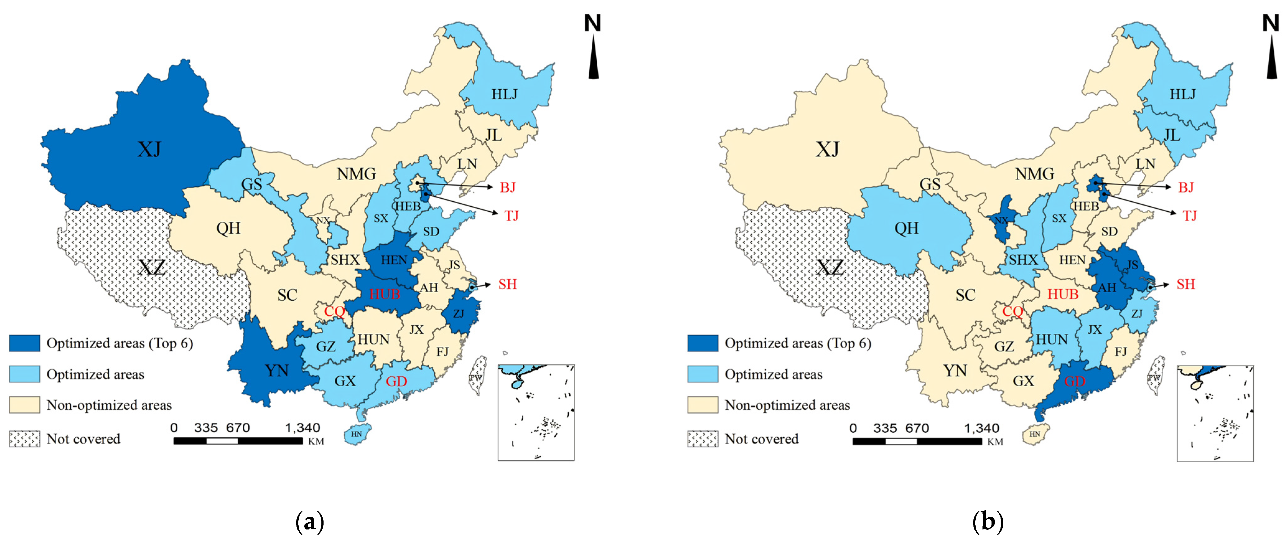
3.2.1. The Economic Effects of CETS on Land Use Transition

To analyze the changes in land use transition at the economic dimension in 30 provincial areas in China before and after the implementation of CETS, we plotted Figure 6 based on the sign direction and value magnitude of the indicators, Evolution_Ecopre and Evolution_Ecoafter. Figure 6a reflects the change in land use transition at the economic level before (2010–2012) and during (2013–2014) CETS implementation. On the other hand, Figure 6b reflects this change in CETS implementation (2013–2014) versus post-implementation (2015–2017) in which optimized areas means that the land use transition has been optimized at the economic level during that time period. In addition, we have highlighted the top six areas with the highest degree of optimization (numerical improvement). The areas marked in red in the figure are the six CETS provincial pilot areas. All areas are marked with abbreviations. Please refer to Table A1 in the Appendix A for the full names.
Figure 6a shows that during the implementation of the policy, there is a significant change in land use transition at the economic level in each province of China, and this change is characterized by spatial clustering (centered on the pilot areas, below). Optimized areas are mainly located in the major urban agglomerations and their radius. Specifically, the Beijing–Tianjin–Hebei urban agglomeration (centered on BJ and TJ), the Yangtze River Delta urban agglomeration (centered on SH), and the Pearl River Delta urban agglomeration (centered on GD) are three of the most important urban agglomerations in China. On the other hand, BJ and CQ, as pilot areas, are non-optimized areas, which indicates that the implementation of the CETS policy has not optimized their land use transition at the economic dimension. This also reflects the spatial spillover effect of CETS on land use transition at this stage. However, we find that the impact of the six pilot provinces on their neighboring areas is negative, i.e., if the pilot areas are optimized, their neighboring areas tend not to be optimized.
Figure 6b shows that the land use transition at the economic dimension in Chinese provinces also changed significantly in the years after the policy was implemented. The spatial distribution pattern of optimized areas in Figure 6b is distinctly different from that in Figure 6a. Although the optimized areas are still dominated by three major urban agglomerations, only the Yangtze River Delta urban agglomeration (centered on SH) belongs to the optimized areas as a whole. In contrast, in the Beijing–Tianjin–Hebei urban agglomeration (centered on BJ and TJ) and the Pearl River Delta urban agglomeration (centered on GD), most of the neighboring provinces in the central region belong to non-optimized areas, which is very different from the distribution pattern in Figure 6a. Moreover, in contrast to the scattered distribution of optimized areas in Figure 6a, the optimized areas in Figure 6b are clearly concentrated in the southeast coastal part of China. On the other hand, CQ and HUB, as pilot areas, are non-optimized areas at this stage, which indicates that their land use transition is not optimized at the economic dimension under the continuous influence of CETS, and BJ, TJ and GD are in the top six. Except for SH, the neighboring provinces of the other five pilot regions tend to belong to non-optimized areas.
In conclusion, from a time-series perspective, CETS affects land use transition in the pilot areas at the economic dimension both during and after implementation. This impact is positive overall. From the spatial distribution perspective, the optimized areas do not show a stable distribution pattern, but change from a scattered distribution in Figure 6a to a “southeastern agglomeration” in Figure 5b.

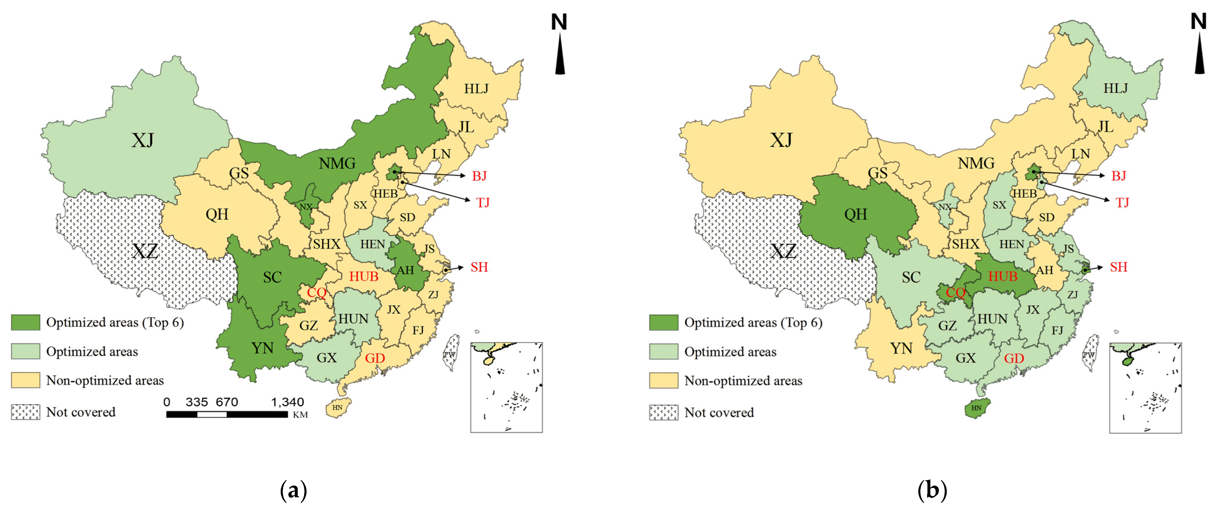
3.2.2. The Environmental Effects of CETS on Land Use Transition

As above, we plot Figure 7 based on the sign direction and value magnitude of the indicators, Evolution_Envpre and Evolution_Envafter. Figure 6 reflects the change in land use transition at the green development dimension. Figure 7a reflects this change in land use transition at the green development dimension before CETS implementation (2010–2012) versus during (2013–2014), whereas Figure 7b reflects this change in land use transition at the green development dimension during CETS implementation (2013–2014) versus after (2015–2017). The signs in the figures and their meanings are the same as above.
Figure 7a shows that, during the implementation of CETS, the overall land use transition of Chinese provinces did not show significant changes at the green development dimension, and there are no obvious spatial clustering characteristics (centered on the pilot areas, the same below). Among the six pilot areas, the rest of the areas did not change significantly under the influence of CETS at this stage, and only BJ belongs to optimized areas and ranks in the top six. In addition, non-optimized areas can be found to be mainly distributed in the eastern and central regions of China.
Figure 7b shows that in the years after the implementation of CETS, the land use transition of each province has changed significantly at the dimension of green development, and there are spatial clustering characteristics. Optimized areas are mainly located in the major urban agglomerations and their radiation areas. Specifically, the four urban agglomerations are Beijing–Tianjin–Hebei (centered on BJ and TJ), the Yangtze River Delta (centered on SH), the Pearl River Delta (centered on GD), and Chengdu–Chongqing (centered on SC and CQ). Moreover, it can be noted that all pilot areas are optimized areas and BJ, SH, HUB and CQ are in the top six optimization levels. This indicates that CETS continues to influence the green development of the pilot areas. On the other hand, it can be found that except for BJ and TJ in the Beijing–Tianjin–Hebei urban agglomeration, which have negative spillover effects on neighboring provinces, the rest of the pilot areas have positive spillover effects on neighboring provinces in general. In addition, the optimized areas in Figure 7b are concentrated in eastern and southern China with a clear distribution pattern.
From a time-period perspective, the impacts of CETS on land use transition are distinct in the two stages illustrated in Figure 6. In the first stage (exhibited in Figure 7a), the CETS implementation process cannot have a significant impact on land use transition from the green development dimension. In contrast, in the second stage (exhibited in Figure 7b), all six pilot areas are optimized areas, and four of them are in the top six in terms of optimization. This indicates that the land use transition of the pilot areas was optimized at the green development dimension during the continuous period after the implementation of CETS. In terms of spatial distribution, the optimized areas in the second stage show a clear “eastern and southern clustering” feature.

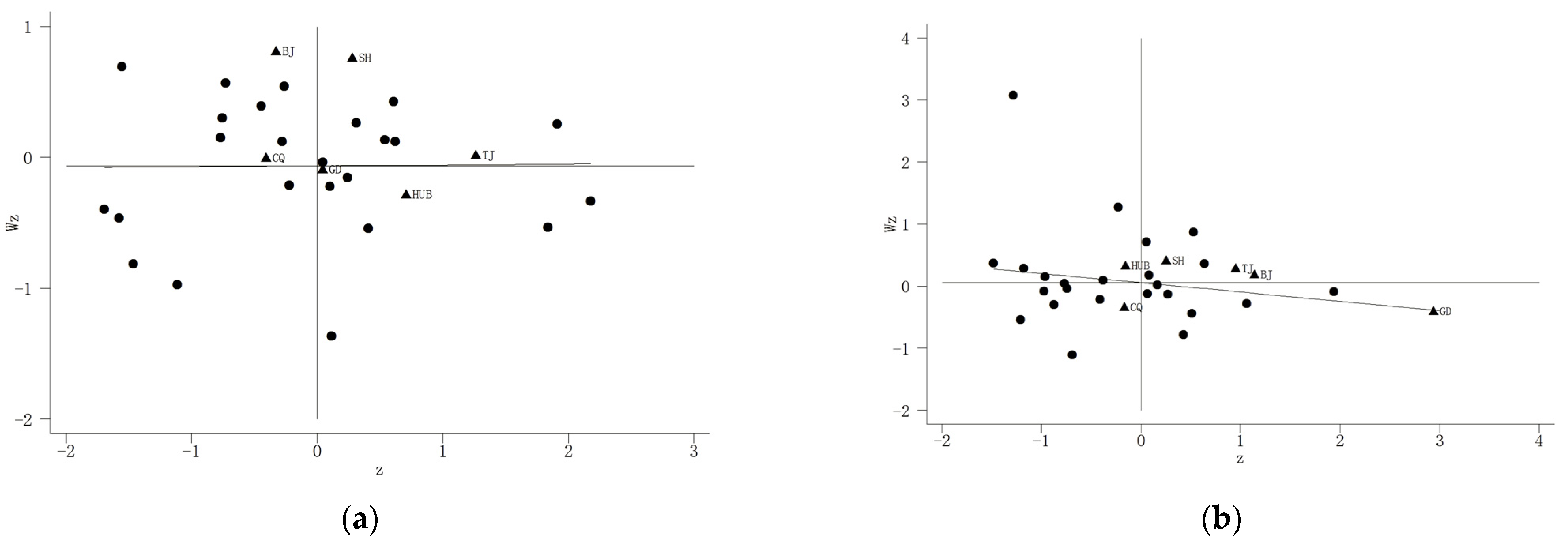
3.3. Test of Spatial Spillover Effects

To further verify the credibility of the results in Figure 6 and Figure 7, a Moran scatterplot is used in this section to determine the spatial clustering characteristics and their spillover effects presented by the six pilot areas in the previous paper at two stages. A Moran scatterplot can better determine the local spatial autocorrelation of the pilot regions. In this study, a Moran scatterplot (Figure 8 and Figure 9) was drawn using the first-order adjacency spatial weight matrix and the four Evolution indicators constructed in Section 2.3.1. These plots can better reflect the spatial influence of the CETS pilot area on its neighboring areas.

3.3.1. Test for Spillover Effects from the Economic Effects of CETS

Figure 8a shows that the negative values of Evolution_Ecopre for BJ and CQ indicate that they are not optimized. The positive values of Evolution_Ecopre for TJ, SH, HUB and GD indicate that they are optimized. Among them, TJ and SH are in the first quadrant (H-H), indicating that they have positive spillover effects. On the other hand, GD and HUB are in the fourth quadrant (H-L), indicating that they produce negative spillover effects, but to a lesser extent. This is more consistent with the results in Section 3.2.1, indicating that the previous results pass the test and are robust.
Figure 8b shows that the Evolution_Ecopost of HUB and CQ are negative, indicating that they are not optimized in this stage. The Evolution_Ecopost of BJ, TJ, SH and GD are positive. Among them, BJ, TJ and SH are in the first quadrant (H-H), indicating that they produce positive spillover effects. GD is in the fourth quadrant (H-L), indicating that they have negative spillover effects, but to a lesser extent. This is more consistent with the results in Section 3.2.1, indicating that the previous results pass the test and are robust.
Therefore, the results of this paper in Section 3.2.1 are robust. Meanwhile, the extent of spillover effects generated by the remaining pilot regions is smaller, except for BJ in the first stage and SH in the second stage. The CQ region is not affected by the economic effects of CETS in both stages.

3.3.2. Test for Spillover Effects from the Environmental Effects of CETS

In Figure 9a, only BJ has a positive value of the Evolution_Envpre, indicating that the green development dimension of land use transition in BJ is optimized. However, BJ is in the fourth quadrant (H-L), reflecting its negative spillover effect on neighboring provinces, but not to a great extent. This is more consistent with the results in Section 3.2.2, indicating that the previous results pass the test and are robust.
In Figure 9b, Evolution_Envpost is positive for all the pilot regions, indicating that the green development dimension of land use transition in the pilot regions is significantly optimized at this stage. Among them, GD, CQ, SH and TJ are in the first quadrant (H-H), reflecting their positive spillover effects on neighboring provinces, and to a larger extent (especially TJ). BJ and HUB are in the fourth quadrant (H-L), reflecting a negative spillover effect on neighboring provinces, but to a lesser extent. This is consistent with the results in Section 3.2.2, indicating that the previous results pass the test and are robust.
Therefore, the results of this paper in Section 3.2.2 are robust. Moreover, it can be found that BJ, which exhibited negative spillover effects in the first stage, produced positive spillover effects in the second stage.

4. Discussion and Policy Inspiration

4.1. Discussion on Hypothesis 1

Figure 5a shows that the secondary indicator of land use transition in terms of economic growth has a small weighting, with the highest weighting summing to less than 20%. This suggests that the change in land use transition originates mainly at the qualitative level of the economy and reflects the changes made by the pilot companies to cater to the CETS and that this behavior has not significantly affected the total local output.
From the results of Section 3, hypothesis 1a of this study holds true, i.e., the economic effect generated by CETS optimizes land use transition in the pilot areas in an economic dimension. In terms of the entire study interval, only CQ was not significantly optimized, while the rest of the areas were optimized by CETS at different stages. Specifically, in the first phase (2010–2014), TJ, SH, HUB and GD were all optimized in the economic dimension, whereas BJ and CQ were not. In the second phase (2013–2017), however, BJ became the optimized area and HUB became the non-optimized area. In short, SH, TJ and GD were optimized throughout, and the optimization was fast and immediate. However, BJ and HUB were only optimized at one stage, with the former being optimized during the second stage and the latter during the first. This reflects the fact that different pilot areas are affected by CETS in different ways due to their specificity. This is particularly true for the speed at which the optimization effect takes effect. Therefore, hypothesis 1b of this study holds true.
We develop the following analysis of the spillover effects in the pilot areas. In the first stage, we cannot draw clear conclusions from Figure 6a, but according to the Moran scatterplot of Figure 8a, we can find that TJ and SH are located in the first quadrant, generating a positive spillover effect, i.e., the land use transition in the region is optimized and the land use transition in the neighboring areas is also optimized. GD and HUB are located in the fourth quadrant and have a negative spillover effect. No spillover effects were observed in the remaining areas. In the second stage, combining the Moran scatterplot of Figure 6b and Figure 8b, we can find that SH, BJ and TJ are in the first quadrant and have a positive spillover effect. GD is in quadrant 4 and has a negative spillover effect on neighboring provinces. Thus, overall, hypothesis 1c holds.
In the context of reality, we discuss some special cases in the conclusions of this paragraph: (1) BJ, as the political center of China, is supposed to be very sensitive to policy, but has not been optimized in the first phase. This is most likely due to its own high economic level (LUpre and LUin values in the top 10%) and the bottleneck in its promotion. (2) CQ was not significantly optimized in either phase, probably because it is the number one electronics and information industry cluster in China and this industry is a major part of its economic output and is not susceptible to the CETS, so land use transition in CQ did not change significantly under the economic effects of the CETS. (3) In the second stage, in addition to BJ and TJ, positive spillover effects were generated in SH, but negative spillover effects were generated in GD. This is because SH is the financial center of China, with fewer polluting industries per se and its output as a share of GDP is limited. In contrast, the tertiary sector, led by the financial sector, accounts for 60–70% of GDP, so SH, under the influence of CETS, not only does not cause negative spillover effects (e.g., the “siphon effect”) to neighboring regions, but also provides them with richer financial services and promotes their economic optimization. In contrast, the secondary sector in GD, which accounts for about 50% of the GDP, is more affected by the CETS, and GD may siphon off more capital to improve its innovation capacity in order to meet the CETS, dragging down the innovation development of neighboring regions. Thus, this creates a negative spillover effect on neighboring regions.

4.2. Discussion on Hypothesis 2

Figure 5b shows that the secondary indicator of land use transition in terms of governance initiatives has a small weighting, with the highest weighting summing up to nearly 30%. This indicates that the change in land use transition is mainly at the level of pollution emissions and reflects that the pilot companies are indeed fulfilling their emission reduction directives. Certainly, industrial output efficiency shows a slow upward trend after 2013, suggesting that one of the results of the feedback from companies as CETS is implemented is an increase in economic output per unit of energy consumed.
From the results of Section 3, hypothesis 2a of this study holds true, i.e., the environmental effects generated by CETS optimize the land use transition of the pilot areas in terms of the green development dimension. In the first phase, only BJ belongs to the optimized area, which may be due to the time lag of the pilot companies in changing their business strategies, mobilizing capital, developing innovations, etc. BJ, on the other hand, as the political center of China, is the most responsive and sensitive to policy. In the second phase, all the pilot areas are optimized areas. Based on this, we can assume that hypothesis 2b is valid. That is, there is a lag in the environmental effects of CETS on land use transition. At the same time, this lag will be changed by the specificity of the pilot areas themselves.
The analysis of spillover effects in the pilot areas is developed as follows. In the first stage, Figure 7a clearly demonstrates that BJ has a negative spillover effect on neighboring provinces. This finding is also tested by the Moran scatterplot in Figure 9a. In the second stage, spillover effects were generated in all pilot areas. Among them, the spillover effect is negative for BJ and HUB and positive for the rest of the regions. Moreover, it can be noted that the values of TJ and the x-axis are significantly larger than those of the y-axis, which indicates a higher degree of positive spillover effects. Based on this, hypothesis 2c is valid in the overall context. However, the sign of the spillover effect depends on the actual situation.
In the context of reality, we discuss some special cases in the conclusions of this paragraph: (1) we find that BJ has continuously transferred a large number of polluting industries to the neighboring province HEB between 2013 and 2017, which explains why only BJ was subject to the optimizing effect of CETS in the first stage and why its spillover effect was negative. (2) In the second stage, TJ, SH, CQ and GD are all located in the first quadrant of the Moran scatterplot, indicating that they generate positive spillover effects. SH, as the financial center of China, has a well-developed tertiary industry, and it is not difficult to achieve pollution reduction. GD’s secondary sector, although well developed, has a “siphoning effect” (from Section 4.1) on the capital of neighboring provinces, which can also help companies to innovate and transform more quickly. The case of CQ is similar to that of GD, with the largest spillover effect in TJ, probably due to the continued transfer of polluting industries from its neighbor BJ to HUB. At the same time, TJ is a region with a predominantly tertiary industry and a secondary industry that is mostly low-polluting and high-tech, and therefore does not have an impact on HEB similar to that of BJ.

4.3. Policy Implication

To summarize this paper, we have reached the following conclusions: Firstly, CETS can optimize land use transition in the pilot areas through economic and environmental effects. However, the effective period of this optimization varies. On the whole, the optimization effect of the economic effect takes effect quickly, while the optimization effect of the environmental effect takes effect slowly. Secondly, there is a spatial spillover effect on the optimization of land use transition by CETS. Moreover, the sign of the spillover effect from both the economic and environmental effects of CETS is not consistent but is related to the industrial structure and development plan of the pilot areas.
Based on the previous analysis and discussion, the following policy implication is obtained from this study: firstly, the implementation of the CETS policy has been relatively successful and is one of the milestones on the road to sustainable development in China. However, the CETS also has many shortcomings that need to be improved. One of the most important issues is that the CETS has not been well tailored to the actual situation in the pilot areas in order to achieve the consistency of policy impact. As a pilot policy, the CETS is bound to evolve into a national policy on carbon emissions reduction, and policies that are not well tailored to local realities will pose many problems, given that the roots of China’s different regions (economic, cultural, environmental, etc.) are very different. Secondly, CETS has not only stimulated innovative R&D behavior of the pilot enterprises, but has also improved the efficiency of industrial output and reduced emissions. Therefore, the central government and local governments should further remove barriers for enterprises to engage in green innovation. For example, they should promote and improve the development of industry–academia–research integration and provide special funding.

Author Contributions

Conceptualization, P.W. (Peijia Wang) and P.W. (Ping Wang); methodology, P.W. (Peijia Wang) and P.W. (Ping Wang); software, P.W. (Peijia Wang); formal analysis, P.W. (Peijia Wang) and P.W. (Ping Wang); writing—original draft preparation, P.W. (Peijia Wang); writing—review and editing, P.W. (Ping Wang). All authors have read and agreed to the published version of the manuscript.

Funding

This research received no external funding.

Institutional Review Board Statement

Not applicable.

Informed Consent Statement

Not applicable.

Data Availability Statement

Raw data on carbon emissions are from CEADs (https://www.ceads.net/ (accessed on 8 August 2021)), whereas other data are mainly from CNRDS (https://www.cnrds.com/ (accessed on 8 December 2021)). We only have the right to use the data and cannot share and upload them publicly. Therefore, the corresponding authors can be contacted for access if needed.

Conflicts of Interest

The authors declare no conflict of interest.

Appendix A

Table A1. Abbreviations of Chinese provincial regions and their corresponding full names.
AbbreviationsFull NameAbbreviationsFull Name
AHAnhui ProvinceJXJiangxi Province
BJBeijing CityLNLiaoning Province
CQChongqing CityNMGInner Mongolia Autonomous Region
FJFujian ProvinceNXNingxia Hui Autonomous Region
GDGuangdong ProvinceQHQinghai Province
GSGansu ProvinceSCSichuan Province
GXGuangxi ProvinceSDShandong Province
GZGuizhou ProvinceSHShanghai City
HEBHebei ProvinceSHXShaanxi Province
HENHenan ProvinceSXShanxi Province
HLJHeilongjiang ProvinceTJTianjin Province
HNHainan ProvinceTWTaiwan Province
HUBHubei ProvinceXJXinjiang Uygur Autonomous Region
HUNHunan ProvinceXZTibet Autonomous Region
JLJilin ProvinceYNYunnan Province
JSJiangsu ProvinceZJZhejiang Province

References

  1. Liu, X.; Zou, B.; Feng, H.; Liu, N.; Zhang, H. Anthropogenic factors of PM2.5 distributions in China’s major urban agglomerations: A spatial-temporal analysis. J. Clean. Prod. 2020, 264, 121709. [Google Scholar] [CrossRef]
  2. Ethan, C.J.; Mokoena, K.K.; Yu, Y.; Shale, K.; Fan, Y.; Rong, J.; Liu, F. Association between PM2.5 and mortality of stomach and colorectal cancer in Xi’an: A time-series study. Environ. Sci. Pollut. Res. 2020, 27, 22353–22363. [Google Scholar] [CrossRef] [PubMed]
  3. Li, H.; Lu, J.; Li, B. Does pollution-intensive industrial agglomeration increase residents’ health expenditure? Sustain. Cities Soc. 2020, 56, 102092. [Google Scholar] [CrossRef]
  4. Liu, L.; Chen, C.; Zhao, Y.; Zhao, E. China’s carbon-emissions trading: Overview, challenges and future. Renew. Sustain. Energy Rev. 2015, 49, 254–266. [Google Scholar] [CrossRef]
  5. Liu, H.; Wang, Y.; Jiang, J.; Wu, P. How green is the “Belt and Road Initiative”?—Evidence from Chinese OFDI in the energy sector. Energy Policy 2020, 145, 111709. [Google Scholar] [CrossRef]
  6. Tang, Y.; Wang, K.; Ji, X.; Xu, H.; Xiao, Y. Assessment and Spatial-Temporal Evolution Analysis of Urban Land Use Efficiency under Green Development Orientation: Case of the Yangtze River Delta Urban Agglomerations. Land 2021, 10, 715. [Google Scholar] [CrossRef]
  7. Guo, X.; Fang, C. Integrated Land Use Change Related Carbon Source/Sink Examination in Jiangsu Province. Land 2021, 10, 1310. [Google Scholar] [CrossRef]
  8. Cao, J.; Karplus, V.J. Firm-level determinants of energy and carbon intensity in China. Energy Policy 2014, 75, 167–178. [Google Scholar] [CrossRef]
  9. Stern, N. A Blueprint for a Safer Planet: How to Manage Climate Change and Create a New Era of Progress and Prosperity; Random House: New York, NY, USA, 2009. [Google Scholar]
  10. Ba, F.; Thiers, P.R.; Liu, Y. The evolution of China’s emission trading mechanisms: From international offset market to domestic Emission Trading Scheme. Environ. Plan. C Politics Space 2018, 36, 1214–1233. [Google Scholar] [CrossRef]
  11. Tang, Y.; Yang, Y.; Xu, H. The Impact of China Carbon Emission Trading System on Land Use Transition: A Macroscopic Economic Perspective. Land 2022, 11, 41. [Google Scholar] [CrossRef]
  12. Ji, X.; Wang, K.; Ji, T.; Zhang, Y.; Wang, K. Coupling Analysis of Urban Land Use Benefits: A Case Study of Xiamen City. Land 2020, 9, 155. [Google Scholar] [CrossRef]
  13. Wang, K.; Tang, Y.; Chen, Y.; Shang, L.; Ji, X.; Yao, M.; Wang, P. The Coupling and Coordinated Development from Urban Land Using Benefits and Urbanization Level: Case Study from Fujian Province (China). Int. J. Environ. Res. Public Health 2020, 17, 5647. [Google Scholar] [CrossRef] [PubMed]
  14. Askariyeh, M.H.; Venugopal, M.; Khreis, H.; Birt, A.; Zietsman, J. Near-Road Traffic-Related Air Pollution: Resuspended PM2.5 from Highways and Arterials. Int. J. Environ. Res. Public Heal. 2020, 17, 2851. [Google Scholar] [CrossRef] [PubMed]
  15. Liu, Y.; Lei, J.; Zhang, Y. A Study on the Sustainable Relationship among the Green Finance, Environment Regulation and Green-Total-Factor Productivity in China. Sustainability 2021, 13, 11926. [Google Scholar] [CrossRef]
  16. De Jong, L.; De Bruin, S.; Knoop, J.; van Vliet, J. Understanding land-use change conflict: A systematic review of case studies. J. Land Use Sci. 2021, 16, 223–239. [Google Scholar] [CrossRef]
  17. Polasky, S.; Kling, C.L.; Levin, S.A.; Carpenter, S.R.; Daily, G.C.; Ehrlich, P.R.; Heal, G.M.; Lubchenco, J. Role of economics in analyzing the environment and sustainable development. Proc. Natl. Acad. Sci. USA 2019, 116, 5233–5238. [Google Scholar] [CrossRef] [Green Version]
  18. Yandri, P.; Priyarsono, D.S.; Fauzi, A.; Dharmawan, A.H. Contemporary Studies on Suburban (Indonesia) Today: Critique on Classical-Neoclassical Regional Economics Based Institutional Economics Perspectives. J. Ekon. Pembang. 2018, 19, 80. [Google Scholar] [CrossRef] [Green Version]
  19. Zilberman, D. Agricultural Economics as a Poster Child of Applied Economics: Big Data & Big Issues 1. Am. J. Agric. Econ. 2019, 101, 353–364. [Google Scholar]
  20. Grainger, A. The Future Role of the Tropical Rain Forests in the World Forest Economy; University of Oxford: Oxford, UK, 1986. [Google Scholar]
  21. Grainger, A. The forest transition: An alternative approach. Area 1995, 27, 242–251. [Google Scholar]
  22. Mather, A.S.; Fairbairn, J.; Needle, C.L. The course and drivers of the forest transition: The case of France. J. Rural Stud. 1999, 15, 65–90. [Google Scholar] [CrossRef]
  23. Mather, A.S.; Needle, C.L. The forest transition: A theoretical basis. Area 1998, 30, 117–124. [Google Scholar] [CrossRef]
  24. Tuan, Y.F. Geography, phenomenology and the study of human nature. Can. Geogr. 1971, 15, 181–192. [Google Scholar] [CrossRef]
  25. Long, H.L. Land Use Transitions and Rural Restructuring in China; Springer: Singapore, 2020. [Google Scholar]
  26. Wen, Y.; Zhang, Z.; Liang, D.; Xu, Z. Rural residential land transition in the Beijing-Tianjin-Hebei region: Spatial-temporal patterns and policy implications. Land Use Policy 2020, 96, 104700. [Google Scholar] [CrossRef]
  27. Tong, W.; Kazak, J.; Qi, H.; Vries, B.D. A framework for path-dependent industrial land transition analysis using vector data. Eur. Plan. Stud. 2019, 27, 1391–1412. [Google Scholar]
  28. Lambin, E.F.; Meyfroidt, P. Land use transition: Socio-ecological feedback versus socio-economic change. Land Use Policy 2010, 27, 108–118. [Google Scholar] [CrossRef]
  29. Long, H.L.; Qu, Y. Land use transitions and land management: A mutual feedback perspective. Land Use Policy 2017, 34, 1607–1618. [Google Scholar] [CrossRef]
  30. Long, H.; Li, T. The coupling characteristics and mechanism of farmland and rural housing land transition in China. J. Geogr. Sci. 2012, 22, 548–562. [Google Scholar] [CrossRef]
  31. Yang, Y.; Bao, W.; Li, Y.; Wang, Y.; Chen, Z. Land use transition and its eco-environmental effects in the Beijing–Tianjin–Hebei urban agglomeration: A production–living–ecological perspective. Land 2020, 9, 285. [Google Scholar] [CrossRef]
  32. Amin, A.; Fazal, S.; Mujtaba, A.; Singh, S.K. Effects of land transformation on water quality of Dal Lake, Srinagar, India. J. Indian Soc. Remote Sens. 2014, 42, 119–128. [Google Scholar] [CrossRef]
  33. Asabere, S.B.; Acheampong, R.A.; Ashiagbor, G.; Beckers, S.C.; Keck, M.; Erasmi, S.; Schanze, J.; Sauer, D. Urbanization, land use transformation and spatio-environmental impacts: Analyses of trends and implications in major metropolitan regions of Ghana. Land Use Policy 2020, 96, 104707. [Google Scholar] [CrossRef]
  34. Liu, Y.Q.; Long, H.L. Land use transitions and their dynamic mechanism: The case of the Huang-Huai-Hai Plain. J. Geogr. Sci. 2016, 26, 515–530. [Google Scholar] [CrossRef] [Green Version]
  35. Van Vliet, J.; de Groot, H.L.F.; Rietveld, P.; Verburg, P.H. Manifestations and underlying drivers of agricultural land use change in Europe. Landsc. Urban Plan 2015, 133, 24–36. [Google Scholar] [CrossRef] [Green Version]
  36. Jin, X.; Xu, X.; Xiang, X.; Bai, Q.; Zhou, Y. System-dynamic analysis on socio-economic impacts of land consolidation in China. Habitat Int. 2016, 56, 166–175. [Google Scholar] [CrossRef]
  37. Faiz, M.A.; Liu, D.; Fu, Q.; Naz, F.; Hristova, N.; Li, T.; Niaz, M.A.; Khan, Y.N. Assessment of dryness conditions according to transitional ecosystem patterns in an extremely cold region of China. J. Clean. Prod. 2020, 255, 120348. [Google Scholar] [CrossRef]
  38. Tang, K.; Liu, Y.; Zhou, D.; Qiu, Y. Urban carbon emission intensity under emission trading system in a developing economy: Evidence from 273 Chinese cities. Environ. Sci. Pollut. Res. 2021, 28, 5168–5179. [Google Scholar] [CrossRef]
  39. Yang, X.; Jiang, P.; Pan, Y. Does China’s carbon emission trading policy have an employment double dividend and a Porter effect? Energy Policy 2020, 142, 111492. [Google Scholar] [CrossRef]
  40. Zhang, Y.; Li, S.; Luo, T.; Gao, J. The effect of emission trading policy on carbon emission reduction: Evidence from an integrated study of pilot regions in China. J. Clean. Prod. 2020, 265, 121843. [Google Scholar] [CrossRef]
  41. Hu, Y.; Ren, S.; Wang, Y.; Chen, X. Can carbon emission trading scheme achieve energy conservation and emission reduction? Evidence from the industrial sector in China. Energy Econ. 2020, 85, 104590. [Google Scholar] [CrossRef]
  42. Froese, R.; Schilling, J. The Nexus of Climate Change, Land Use, and Conflicts. Curr. Clim. Change Rep. 2019, 5, 24–35. [Google Scholar] [CrossRef] [Green Version]
  43. Ge, D.; Wang, Z.; Tu, S.; Long, H.; Yan, H.; Sun, D.; Qiao, W. Coupling analysis of greenhouse-led farmland transition and rural transformation development in China’s traditional farming area: A case of Qingzhou City. Land Use Policy 2019, 86, 113–125. [Google Scholar] [CrossRef]
  44. Chang, B.; Chen, L. Land Economic Efficiency and Improvement of Environmental Pollution in the Process of Sustainable Urbanization: Case of Eastern China. Land 2021, 10, 845. [Google Scholar] [CrossRef]
  45. Liu, Y.; Long, H.; Li, T.; Tu, S. Land use transitions and their effects on water environment in Huang-Huai-Hai Plain, China. Land Use Policy 2015, 47, 293–301. [Google Scholar] [CrossRef]
  46. Turner, B.L.; Lambin, E.F.; Reenberg, A. The emergence of land change science for global environmental change and sustainability. Proc. Natl. Acad. Sci. USA 2007, 104, 20666–20671. [Google Scholar] [CrossRef] [PubMed] [Green Version]
  47. Lv, M.; Bai, M. Evaluation of China’s carbon emission trading policy from corporate innovation. Financ. Res. Lett. 2021, 39, 101565. [Google Scholar] [CrossRef]
  48. Duan, B.; Ji, X. Can Carbon Finance Optimize Land Use Efficiency? The Example of China’s Carbon Emissions Trading Policy. Land 2021, 10, 953. [Google Scholar] [CrossRef]
  49. Xia, Q.; Li, L.; Dong, J.; Zhang, B. Reduction Effect and Mechanism Analysis of Carbon Trading Policy on Carbon Emissions from Land Use. Sustainability 2021, 13, 9558. [Google Scholar] [CrossRef]
  50. Moulds, S.; Buytaert, W.; Mijic, A. A spatio-temporal land use and land cover reconstruction for India from 1960–2010. Sci. Data 2018, 5, 180159. [Google Scholar] [CrossRef]
  51. Aburas, M.M.; Ahamad, M.S.S.; Omar, N.Q. Spatio-temporal simulation and prediction of land-use change using conventional and machine learning models: A review. Environ. Monit. Assess. 2019, 191, 205. [Google Scholar] [CrossRef]
  52. Xu, H.; Shi, X.; Wang, K. The Influence of Absorptive Capacity on Regional Innovation—An Empirical Research Based on Knowledge Spillovers. J. Jimei Univ. (Philos. Soc. Sci.) 2018, 21, 49–55. [Google Scholar] [CrossRef]
  53. Tobler, W.R. A computer movie simulating urban growth in the Detroit region. Econ. Geogr. 1970, 46, 234–240. [Google Scholar] [CrossRef]
  54. Du, G.; Yu, M.; Sun, C.; Han, Z. Green innovation effect of emission trading policy on pilot areas and neighboring areas: An analysis based on the spatial econometric model. Energy Policy 2021, 156, 112431. [Google Scholar] [CrossRef]
  55. Li, D.; Liu, L.; Wang, H. The U curve of labor share in GDP during economic development. Econ. Res. J. 2009, 1, 362–382. [Google Scholar]
  56. Kuznets, S. Quantitative Aspects of the Economic Growth of Nations: II. Industrial Distribution of National Product and Labor Force. Econ. Dev. Cult. Change 1957, 5, 1–111. [Google Scholar] [CrossRef]
  57. Brunnermeier, S.B.; Cohen, M.A. Determinants of environmental innovation in US manufacturing industries. J. Environ. Econ. Manag. 2003, 45, 278–293. [Google Scholar] [CrossRef]
  58. Ashford, N.A.; Hall, R.P. The Importance of Regulation-Induced Innovation for Sustainable Development. Sustainability 2011, 3, 270–292. [Google Scholar] [CrossRef] [Green Version]
  59. Muthuri, J.N.; Moon, J.; Idemudia, U. Corporate innovation and sustainable community development in developing countries. Bus. Soc. 2012, 51, 355–381. [Google Scholar] [CrossRef]
  60. Wallsten, S.J. The effects of government-industry R&D programs on private R&D: The case of the Small Business Innovation Research program. RAND J. Econ. 2000, 31, 82–100. [Google Scholar]
  61. De Bruyn, S.M.; van den Bergh, J.C.; Opschoor, J.B. Economic growth and emissions: Reconsidering the empirical basis of environmental Kuznets curves. Ecol. Econ. 1998, 25, 161–175. [Google Scholar] [CrossRef]
  62. Qian, Y.; Xu, C. Why China’s economic reforms differ: The M-form hierarchy and entry/expansion of the non-state sector. Econ. Transit. 1993, 1, 135–170. [Google Scholar] [CrossRef] [Green Version]
  63. Gray, W.B.; Shadbegian, R.J. Environmental Regulation, Investment Timing, and Technology Choice. J. Ind. Econ. 1998, 46, 235–256. [Google Scholar] [CrossRef]
  64. Simpson, R.D.; Bradford, I.R.L. Taxing Variable Cost: Environmental Regulation as Industrial Policy. J. Environ. Econ. Manag. 1996, 30, 282–300. [Google Scholar] [CrossRef]
  65. Shan, Y.; Guan, D.; Zheng, H.; Ou, J.; Li, Y.; Meng, J.; Mi, Z.; Liu, Z.; Zhang, Q. China CO2 emission accounts 1997–2015. Sci. Data 2018, 5, 170201. [Google Scholar] [CrossRef] [PubMed] [Green Version]
  66. Shan, Y.; Huang, Q.; Guan, D.; Hubacek, K. China CO2 emission accounts 2016–2017. Sci. Data 2020, 7, 1–9. [Google Scholar] [CrossRef] [PubMed] [Green Version]
  67. Yang, L.; Li, Y.; Liu, H. Did carbon trade improve green production performance? Evidence from China. Energy Econ. 2021, 96, 105185. [Google Scholar] [CrossRef]
  68. Zhang, N.; He, S.D.; Wang, J.F.; Chen, Y.; Kang, L. Carbon Intensity and Benchmarking Analysis of Power Industry in Tianjin under the Context of Cap-and-Trade. Res. Environ. Sci. 2018, 31, 187–193. [Google Scholar]
Figure 1. China’s CO2 emission and change rate.
Land 11 00440 g001
Figure 2. Distribution map of the six pilot regions.
Land 11 00440 g002
Figure 3. Diagram of the study strategy.
Land 11 00440 g003
Figure 4. Diagram of queen contiguity. Spillover effect areas are marked with a “√”.
Land 11 00440 g004
Figure 5. Trends in weight changes of each secondary indicator measured by the entropy method over the years. (a) land use transition measured from the economic dimension; (b) land use transition measured from the green development dimension.
Land 11 00440 g005
Figure 6. Spatio-temporal evolution distribution of land use transition at the economical dimension. (a) Differences between the CETS implementation process and before implementation; (b) differences between the CETS post-implementation and implementation process.
Land 11 00440 g006
Figure 7. Spatio-temporal evolution of land use transition at the green development dimension. (a) Differences between the CETS implementation process and before implementation; (b) differences between the CETS post-implementation and implementation process.
Land 11 00440 g007
Figure 8. Moran scatterplots for the Evolution_Eco indicator. (a) Differences between the CETS implementation process and before implementation; (b) differences between the CETS post-implementation and implementation process.
Land 11 00440 g008
Figure 9. Moran scatterplots for the Evolution_Env indicator. (a) Differences between the CETS implementation process and before implementation; (b) differences between the CETS post-implementation and implementation process.
Land 11 00440 g009
Table 1. Evaluation system of land use transition indicators under the economic and green development dimensions.
DimensionTypeSecondary IndicatorsUnitDirectionObsMeanStd. Dev.MinMax
Economic dimension of land useEconomic growthGDP growth rate%+2409.70 2.80 0.50 17.40
GDP per capita growth rate%+2409.01 3.30 −2.40 25.30
Economic qualityThe proportion of added value of
tertiary industry
%+24045.79 9.09 30.70 82.70
Share of science and technology expenditure%+2401.96 1.38 0.39 6.58
Full-time equivalent of R&D personnelMan-year+2409.70 2.80 0.50 17.40
Green development dimension of land usePollution emissionsIndustrial
waste gas emissions intensity
Thousand tons/km2-2402.303.844.05 × 10−522.01
Industrial
wastewater emissions intensity
Thousand tons/km2-2407.2612.200.1174.51
Industrial soot emissions intensityTons/km2-2403.023.090.1822.49
Carbon dioxide emission intensityThousand tons/km2-2403.386.030.0436.62
Governance InitiativesIndustrial output efficiencyYuan/KWh+2407.82 7.18 0.75 54.58
Share of investment in pollution control%+2401.47 0.74 0.30 4.24
Publisher’s Note: MDPI stays neutral with regard to jurisdictional claims in published maps and institutional affiliations.

