GIS-Based Comparative Study of the Bayesian Network, Decision Table, Radial Basis Function Network and Stochastic Gradient Descent for the Spatial Prediction of Landslide Susceptibility

Abstract

Landslides frequently occur along the eastern margin of the Tibetan Plateau, which poses a risk to the construction, maintenance, and transportation of the proposed Dujiangyan city to Siguniang Mountain (DS) railway, China. Therefore, four advanced machine learning models, namely, the Bayesian network (BN), decision table (DTable), radial basis function network (RBFN), and stochastic gradient descent (SGD), are proposed in this study to delineate landslide susceptibility zones. First, a landslide inventory map was randomly divided into 828 (75%) samples and 276 (25%) samples for training and validation, respectively. Second, the One-R technique was utilized to analyze the importance of 14 variables. Then, the prediction capability of the four models was validated and compared in terms of different statistical indices (accuracy (ACC) and Cohen’s kappa coefficient (k)) and the areas under the curve (AUC) in the receiver operating characteristic curve. The results showed that the SGD model performed best (AUC = 0.897, ACC = 80.98%, and k = 0.62), followed by the BN (AUC = 0.863, ACC = 78.80%, and k = 0.58), RBFN (AUC = 0.846, ACC = 77.36%, and k = 0.55), and DTable (AUC = 0.843, ACC = 76.45%, and k = 0.53) models. The susceptibility maps revealed that the DS railway segments from Puyang town to Dengsheng village are in high and very high-susceptibility zones.

1. Introduction

Landslide phenomena are the response of geomorphic evolution and are common hazardous processes in mountain areas, which frequently cause substantial loss of life and property, as well as considerable damage to the ecological environment around the world [1]. Many scholars have confirmed that increasing landslide events are mainly associated with climate changes, rapid snowmelt, earthquakes, rapid land-use changes, and extensive human activities [2,3], which present considerable challenges to the engineering construction of traffic arteries and water conservancy facilities [4]. With the rapid uplift of the Tibetan Plateau, the internal and external dynamic geological processes are strongly intertwined and transformed, shaping complex and special geological environmental conditions and strong river dynamic processes along this plateau margin [5,6]. Under this geological environmental condition, landslides are extremely well developed along the eastern margin of the Tibetan Plateau (EMTP), causing significant socioeconomic losses and casualties every year [7]. In addition, in the Longmenshan area of the EMTP, the government department is planning to combine rail transit and mountain tourism by building a new railway with toothed rail standards from Dujiangyan city to Siguniang Mountain (DS railway), which will contribute to tourism development and local economic growth [8]. The DS railway is mainly built along the Yuzi River with alpine canyon landforms. The railway crossing region is a special area with complicated geomorphology, great disparity in altitude, a steep gorge, strongly incised river, active tectonic movement, and variety of climates. Notably, landslides are an inevitable problem in the construction of infrastructure, and they seriously restrict and affect the planning, construction, operation and maintenance of DS railway projects. Therefore, to reduce and manage landslide-related disasters, it is vital and worthwhile to create landslide susceptibility maps (LSMs) for delineating landslide-prone zones as references in railway planning [9,10]. Landslide mitigation is also an important step towards achieving the United Nations sustainable development goals [11].

Landslide susceptibility is related to the possibility of landslide occurrence in a given region based on the local environmental conditions [12]. Landslide susceptibility mapping, which depends on topography, geology, geotechnical properties, climate, vegetation, and anthropogenic factors, involves the spatial distribution and rating of the terrain units in accordance with their tendency to generate slope instability. Since the mid-1970s, a significant number of techniques have been employed to study landslide susceptibility [13,14]. These techniques can be categorized into knowledge-based, physically based, bivariate and multivariate statistical, and machine learning (ML) models. Among these models, ML models have gained substantial attention and have been increasingly applied in the landslide susceptibility domain due to their high ability to handle complex and nonlinear data [15]. As reported in previous studies, ML models are more accurate than conventional methods. For example, Yilmaz [16] used frequency ratio (FR), logistic regression (LR), and artificial neural networks (ANN) to compare landslide susceptibility, indicating that the areas under the curve (AUC) value of 0.852 for ANN exceeded those values of the FR and LR models. Goetz, et al. [17] presented a comparison of traditional statistical and ML models applied for regional landslide susceptibility, demonstrating that random forest and bootstrap aggregated classification trees had the overall best predictive performances compared with LR, generalized additive models, and weights of evidence. Similarly, Huang, et al. [18] discovered that the performances of ML models, including the multilayer perceptron, backpropagation neural network, support vector machine (SVM), and C5.0 decision tree (DT), have better prediction accuracy than heuristic and general statistical approaches in Shicheng County, China. In addition, other ML techniques, such as Bayesian algorithms (naïve Bayes (NB) and Bayesian belief network), ANN algorithms (convolutional neural network, recurrent neural network, self-organizing map), and DT algorithms (classification and regression tree, alternating DT, and ID3 DT), are also widely applied to predict landslide susceptibility [15,19,20,21,22].

Nevertheless, each ML model has proven to have its own sole merits and demerits. The prediction capacity of the model depends on the available data, characteristics of the research sites, and scale of the analysis. In addition, the data employed to build landslide susceptibility models usually comprise abundant instances with dozens of attributes [23]. Therefore, using conventional ML methods (e.g., ANN and SVM) to train landslide susceptibility models may take much time and occupy extensive random-access memory. Stochastic gradient descent (SGD) usually selects a random sample to iteratively update the model parameters, resulting in the learning being very fast and can be updated online. Thus, SGD speeds up the convergence rate and shortens the training time. SGD has been successfully applied to solve large-scale and sparse ML problems, which is often encountered in text classification and natural language processing [24]. However, the SGD model has rarely been utilized in landslide prediction. In previous landslide-related studies, we discovered that only Bui, et al. [25] applied the SGD model to predict landslides, while Hong, et al. [26]; Nhu, et al. [27]; and Wang, et al. [28] employed the SGD algorithm to optimize deep learning models. Notably, the SGD model needs to be further explored. Therefore, in this study, the SGD model was introduced to assess landslide susceptibility along the DS railway. Furthermore, to more fully reflect the comprehensive performance of the SGD model, the Bayesian network (BN) and radial basis function network (RBFN) models, two famous supervised learning algorithms, were taken as the reference models in this study. Many scholars have demonstrated the excellent ability of the BN and RBFN models in predicting regional landslide risk. For instance, Song, et al. [29] and Lee, et al. [30] applied the BN model to analyze the spatial prediction of landslide susceptibility and achieved a high probability of landslide detection. Pham, et al. [31] predicted landslide susceptibility in the Van Chan district (Vietnam) by combining an RBFN with the random subspace, attribute selected classifier, cascade generalization, and Dagging. The results indicate that the single RBFN model (AUC = 0.799) outperformed all the ensemble models in the training dataset. In addition, a decision table (DTable), another rarely utilized rule classification algorithm, was also applied to generate LSMs for comparison. Pham, et al. [32] employed the DTable model to predict the susceptibility of landslides and compared it with other state-of-the-art ML models. However, in previous studies, there has been no comparative study of these four advanced models.

Thus, this paper aims to compare the prediction capability of four ML models, namely, BN, DTable, RBFN, and SGD, in landslide susceptibility modeling along the DS railway. The paper also aims to determine the most effective model among the four models by using statistical indices and the receiver operating characteristic (ROC) curve. This study substantially contributes to the ongoing scientific debate on landslide susceptibility modeling and guides the prediction and early warning of landslide disasters along this vital corridor.

2. Study Area and Materials

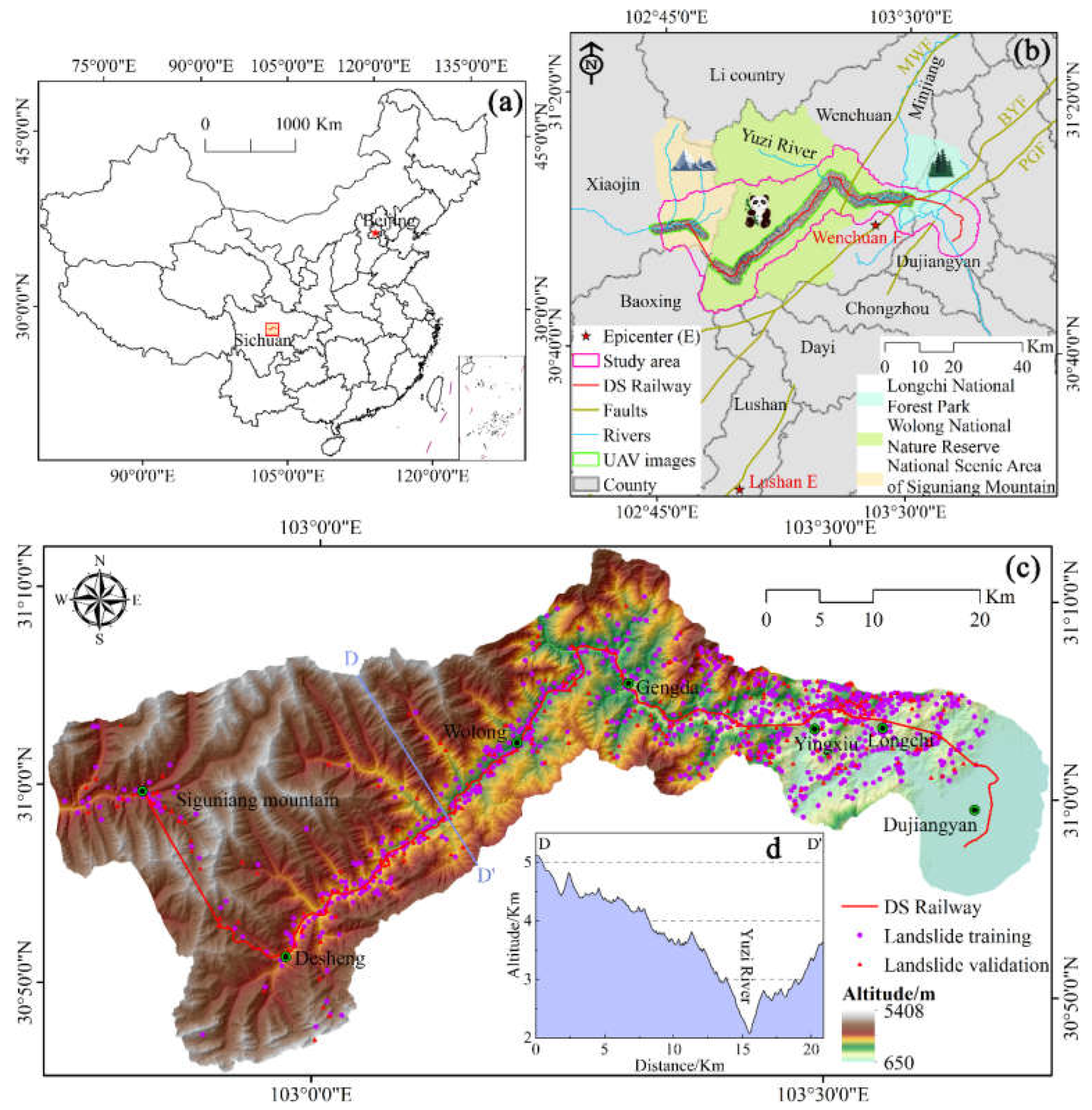
2.1. Study Area

The planned tourist DS railway is in western Sichuan Province, China (Figure 1a). The railway starts in Dujiangyan city, passes through the Longchi National Forest Park and the Wolong National Nature Reserve (a World Natural Heritage Giant Panda Habitat), and ends in the National Scenic Area of Siguniang Mountain, Xiaojin County (Figure 1b,c). The railway spans approximately 123 km, and the total study area is 1813.58 km². In terms of geomorphic units, the study area lies in the EMTP, which is the transition area from the Sichuan Basin with an altitude of 600~700 m to the Tibetan Plateau with an altitude of 3000~5600 m. The landform characteristics mainly consist of plains, hills, mountains, valleys, and ice margins. The tectonic position of the study area is the active suture zone of the Songpan-Ganze orogenic belt and Yangtze Plate [33]. The geological tectonic movement is active, and the overall structural trace is distributed in a northeast-southwest direction. The DS railway spans the Longmenshan fold-and-thrust belt, consisting of the Pengxian-Guanxian faults (PGF), Beichuan-Yingxiu faults (BYF), and Maoxian-Wenchuan faults (MWF), where the Ms 8.0 Wenchuan earthquake and Ms 7.0 Lushan earthquake occurred. Geologically, sedimentary rocks (e.g., sandstone and limestone) are exposed from Dujiangyan city to Yingxiu town. The volcanic rocks (e.g., diorite and granodiorite) crop out from Yingxiu to Gengda towns. The metamorphic rocks (phyllite, metamorphic sandstone, slate, altered basalt, and quartzite) are located from Gengda to Siguniang Mountain towns along the railway route. The rock strata mainly comprise Mesoproterozoic to Cenozoic strata, while Cambrian, Ordovician, Paleogene, and Neogene strata are absent in the study area [8]. Hydrologically, the main rivers in the area are the Minjiang River and its tributary Yuzi River, where the railway mainly runs along the Yuzi River. River incision into bedrock occurs at a rate of 1.81 mm/year [34]. From Dujiangyan to Yingxiu in the eastern part of the study area, the annual rainfall ranges from 920 mm to 1177 mm. From Gengda to Dengsheng, the average annual precipitation is 888 mm/year. At Siguniang Mountain, the annual rainfall ranges from 710 mm to 930 mm.

In total, under the influence of earthquakes, faults, differential weathering, and erosion, the rock mass is mostly fragmented and has poor integrity. These factors, combined with human activities and extreme rainfall, cause the widespread occurrence of landslides in this region.

2.2. Landslide Inventory

An accurate landslide inventory map is vital for predictions in landslide-prone areas and regional landslide prevention. In the present study, a landslide inventory map was prepared based on historical landslide records and manual visual interpretation of 0.15 m resolution unmanned aerial vehicle (UAV) aerial photographs (Figure 1b), ~0.5 m resolution World View-2 and Geoeye-1 satellite images, and 10 m resolution Sentinel-2A satellite images. Extensive field reconnaissance supported by the China Railway Eryuan Engineering Group Co., Ltd. was then conducted for verification (Figure 2). A total of 1104 landslide locations (Figure 1c), which consisted of slides and falls (Figure 2), were mapped and identified [35]. The smallest and largest area dimensions of the landslides identified are 2.28 × 10² and 3.11 × 10⁶ m², respectively. Approximately 1.00%, 19.75%, 55.62% and 23.64% of landslides are characterized as very large-sized (>1 km²), large-sized (0.1–1 km²), medium-sized (0.01–0.1 km²), and small-sized landslides (<0.01 km²), respectively. For landslide spatial analysis, all the landslide polygons were transformed into points and then randomly split into two subsets with 75% (828 landslides) and 25% (276 landslides) for training and validation purposes, respectively. In addition, an equal number of non-landslide points were randomly selected from the landslide-free areas and then divided into a training dataset and a validation dataset with the same proportions.

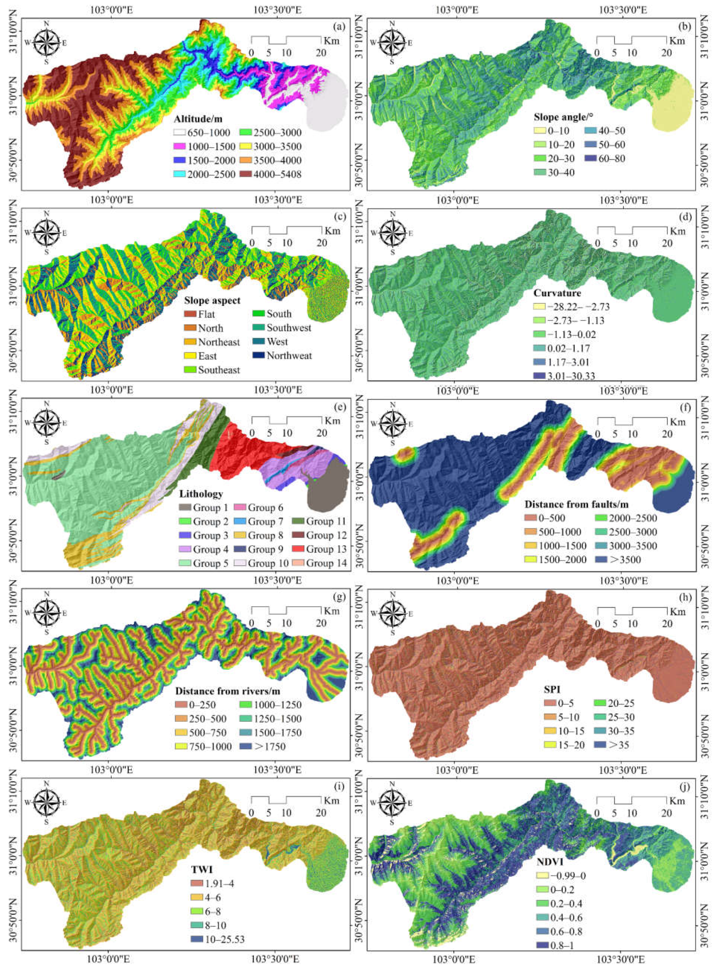
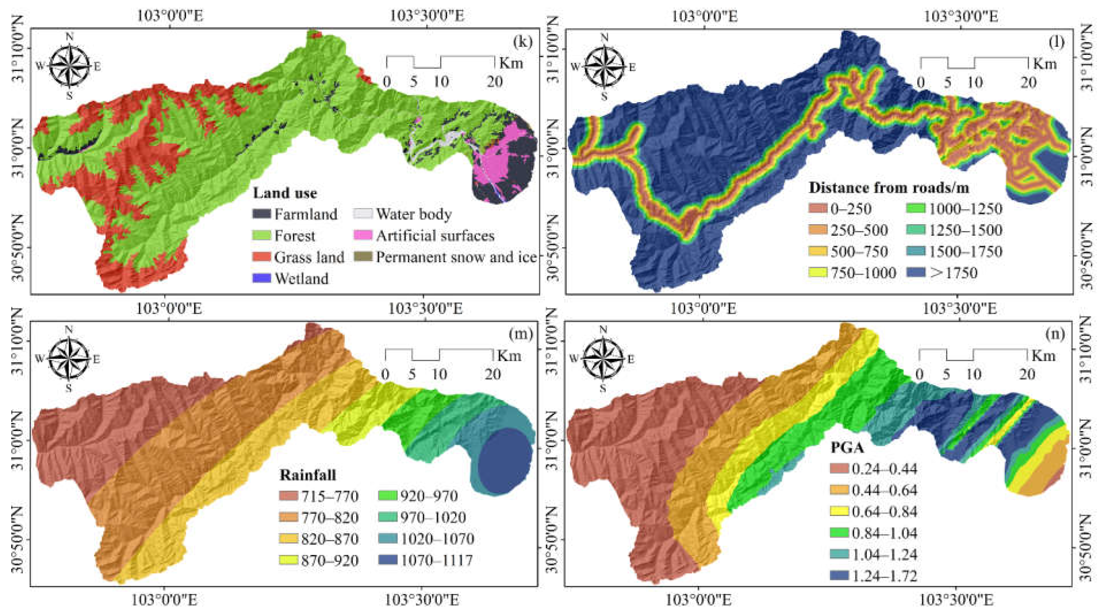
2.3. Landslide-Related Variables

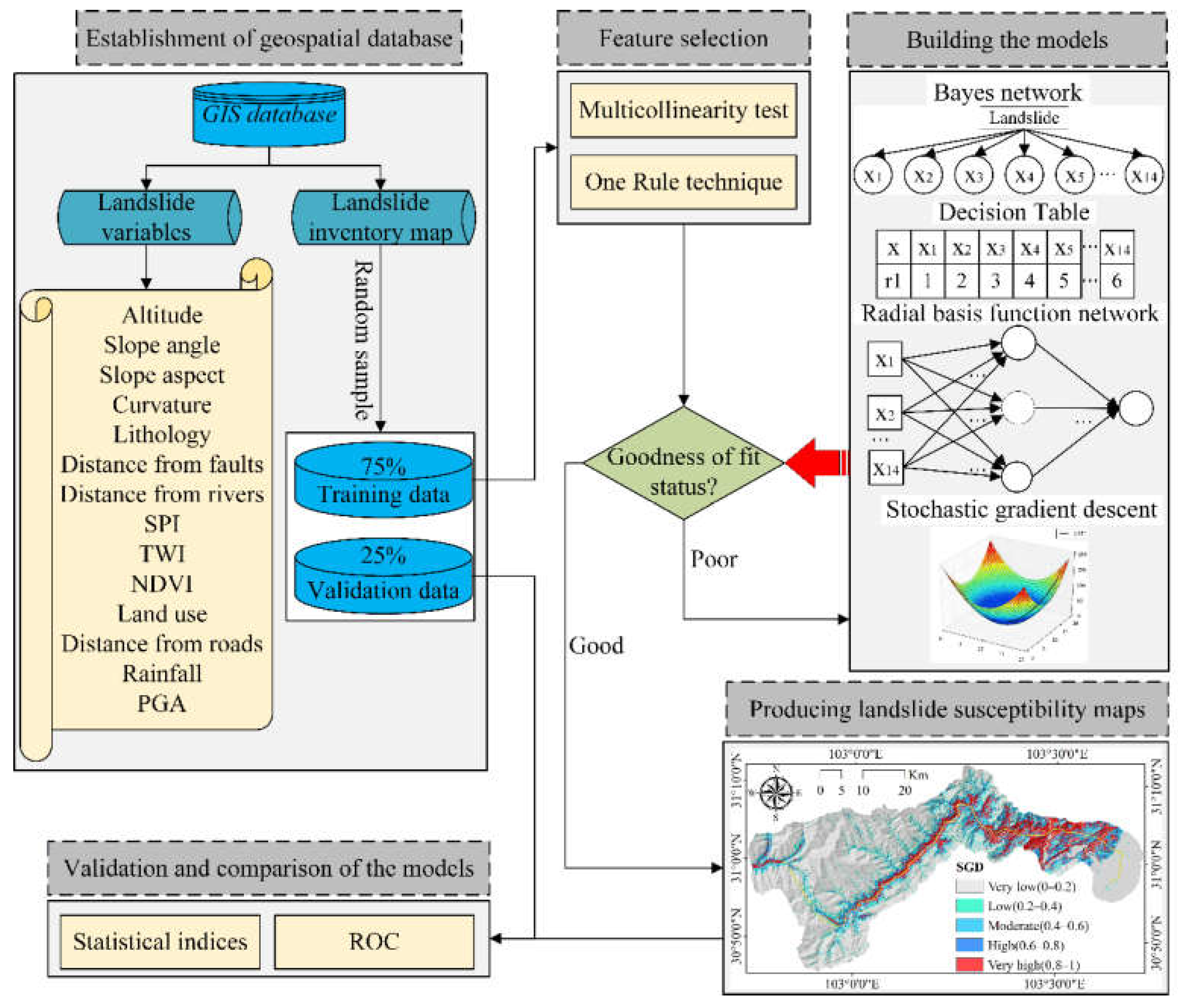
After compiling the landslide inventory map, it is necessary to select and create landslide-related variables in the process of landslide susceptibility modeling [36]. Based on some previous studies and the geological environment features of the study area, 14 variables related to geology, topography, hydrogeology, and the environment were adopted: altitude, slope angle, slope aspect, curvature, lithology, distance from faults, distance from rivers, stream power index (SPI), topographic wetness index (TWI), normalized difference vegetation index (NDVI), land use, distance from roads, rainfall, and peak ground acceleration (PGA). The details of the selected variables are presented in

Table 1. Landslide-related variables and their classes.

Variables	Classes (j)	Descriptions of Variables	Classified Method/Number of Classes (m)	Resolution (Scale)
Altitude/m	650–1000; 1000–1500; 1500–2000; 2000–2500; 2500–3000; 3000–3500; 3500–4000; 4000–5408	Potential energy, vegetation, temperature, rainfall, and human activities always change with altitude, resulting in the development of landslides within a certain range of altitudes.	Equal interval/8	30 × 30 m
Slope angle/°	0–10; 10–20; 20–30; 30–40; 40–50; 50–60; 60–80	Slope angle affects the stress distribution, thickness of loose solid matter, vegetation coverage, and surface water runoff.	Equal interval/7	30 × 30 m
Slope aspect	Flat; N; NE; E; SE; S; SW; W; NW	Slope aspect affects the vegetation cover, water evaporation, and weathering degree of the hillslope.	Equal interval/9	30 × 30 m
Curvature	[(−28.22)–(−2.73)]; [(−2.73)–(−1.13)]; [(−1.13)–0.02]; [0.02–1.17]; [1.17–3.01]; [3.01–30.33]	Curvature affects the internal stress of hillslope and the runoff of surface water.	Natural break/6	30 × 30 m
Lithology	Group 1; group 2; group 3; group 4; group 5; group 6; group 7; group 8; group 9; group 10; group 11; group 12; group 13; group 14	Lithology is the material basis of landslide disasters, which affects the difficulty of hillslope erosion. The group details are shown in Table 2.	Lithofacies/14	1:200,000
Distance from faults/m	0–500; 500–1000; 1000–1500; 1500–2000; 2000–2500; 2500–3000; 3000–3500; >3500	Faults destroy the integrity of rock masses and provide channels for groundwater flow.	Equal interval/8	1:200,000
Distance from rivers/m	0–250; 250–500; 500–750; 750–1000; 1000–1250; 1250–1500; 1500–1750; >1750	The river can erode and soften the hillslope toe, thus reducing the shear strength of the hillslope.	Equal interval/8	30 × 30 m
SPI	0–5; 5–10; 10–15; 15–20; 20–25; 25–30; 30–35; >35	$SPI=A_s\ast \tan \beta$ can describe the potential erosion capacity of water flow at a given location in a watershed, where As is the specific catchment area (m2/m) and β is the slope angle (°).	Equal interval/8	30 × 30 m
TWI	1.94–4; 4–6; 6–8; 8–10; >10	$TWI=Ln(A_s/\tan \beta )$ is an indicator of surface soil moisture, which can quantitatively evaluate the runoff trend and the location of runoff convergence.	Equal interval/5	30 × 30 m
NDVI	(−0.95)–0; 0–0.2; 0.2–0.4; 0.4–0.6; 0.6–0.8; 0.8–1	NDVI has been widely employed to measure the degree of vegetation development, which is related to hillslope runoff, infiltration, and weathering [36].	Equal interval/6	10 × 10 m
Land use	Farmland; forest; grass land; wetland; water bodies; artificial surfaces; permanent snow and ice	Different land-use types have different effects on landslides, and unreasonable land use can aggravate landslides.	Land use unit/7	30 × 30 m
Distance from roads/m	0–250; 250–500; 500–750; 750–1000; 1000–1250; 1250–1500; 1500–1750; >1750	Road construction always influences changing in hillslope geometry, stress and hydrology [37].	Equal interval/8	1:50,000
Rainfall/mm	717–770; 770–820; 820–870; 870–920; 920–970; 970–1020; 1020–1070; 1070–1117	Rainfall can erode the hillslope surface, destroy the surface integrity of rock and soil masses, and reduce the shear strength of rock and soil masses.	Equal interval/8	30 × 30 m
PGA/g	0.24–0.44; 0.44–0.64; 0.64–0.84; 0.84–1.04; 1.04–1.24; 1.24–1.72	One of the main indicators of an earthquake, as well as a direct trigger of seismic landslides [38].	Equal interval/6	30 × 30 m

and Figure 3.

An Advanced Land Observing Satellite (ALOS) digital elevation model (DEM) with a resolution of 30 m (https://www.eorc.jaxa.jp/ALOS, accessed on 4 November 2021) was adopted to derive the topographic and hydrological variables, such as altitude, slope angle, slope aspect, curvature, distance from rivers, SPI, and TWI. In addition, geological variables, such as lithology and fault information, were obtained from the geological map at the 1:200,000 scale provided by the China Geological Survey and rectified from the field survey. The lithology in the study area is grouped into 14 classes based on the geological age, rock type, and geotechnical criteria (Figure 3e and

Table 2. Classification and description of the geological units in the study area.

Classification	Code	Lithology	Geological Age	Area/km2
Group 1	Q2, Q4	Alluvium and colluvial sediments	Quaternary	133.57
Group 2	K2g, K1j	Quartz sandstone, siltstone, and sandy mudstone	Cretaceous	1.31
Group 3	J3l, J2sn, J2s	Sandstone, siltstone, sandy mudstone, and calcareous conglomerate	Jurassic	15.00
Group 4	T3	Conglomerate, feldspathic quartz sandstone, siltstone with shale and thin coal layer	Upper Triassic	120.23
Group 5	T1, T2, T3	Metasandstone, phyllite, crystalline limestone	Triassic	871.64
Group 6	P1	Dolomitic limestone, argillaceous limestone	Permian	14.38
Group 7	C	Limestone intercalated with calcareous shale, mudstone	Carboniferous	8.95
Group 8	C, T	Crystalline limestone, altered basalt, and phyllite	Carboniferous and Triassic	192.52
Group 9	D2, D3	Limestone, dolomite, sandstone, and shale	Devonian	5.07
Group 10	Dwg	Phyllite with quartzite and crystalline limestone	Devonian	149.28
Group 11	Smx	Phyllite, quartzite, crystalline limestone, metamorphic siltstone	Silurian	98.66
Group 12	Za	Andesite, rhyolite, tuff lava, breccia agglomerate	Sinian	11.68
Group 13	γο2(4), γδ2(3), γδ2(4), δο2(3)	Plagioclase granite, diorite, granodiorite, and diabase	Proterozoic	189.24
Group 14	Pthn	Gabbro, diorite and quartz diorite	Proterozoic	2.03

). A land-use map of 2020 with a 30-m spatial resolution was downloaded from the Global Geo-information Public Product website (http://www.globallandcover.com, accessed on 8 November 2021). Land-use types were partitioned to delineate seven types: farmland, forest, grass land, wetland, water bodies, artificial surfaces, and permanent snow and ice. In QGIS software, the NDVI was calculated using two Sentinel-2B images with a 10-m spatial resolution from 14 January 2021, and the orbit number of the images was 20150. Road information was provided by the National Platform for Common Geospatial Information Services (https://www.tianditu.gov.cn, accessed on 7 November 2021). In the Geographic Information System (GIS) environment, the distance from roads was prepared using the Euclidean distance function along the roads (Figure 3l). A mean annual rainfall contour map was generated using the kriging spatial interpolation method in the GIS environment based on annual rainfall data (1981–2010) provided by the China Meteorological Administration. The PGA for the 2008 Ms. 8.0 Wenchuan earthquake was employed in this work and extracted from the United States Geological Survey (USGS).

To avoid uncertainties associated with different spatial resolutions, all relevant variables were converted into raster format with a 30-m resolution using QGIS software, which is conducive to achieving better results [39]. Among these 14 variables, lithology and land use are categorical variables, whereas the other variables are continuous variables. Both categorical and continuous variables can be used for four models. Studies have shown that the use of all categorical variables can yield a more accurate predictive performance than the use of partially continuous variables [40]. In addition, obtaining a standardized variable map is a prerequisite for landslide analysis [41]. Therefore, in the present study, continuous variables were reclassified into categorical variables based on different methods. Based on many previous studies (e.g., [42]), curvature was classified using the natural breaks method, which can form several classes based on the intrinsic features of a dataset without any subjective thought [23]. The other continuous variables were classified using the equal interval method following certain guidelines and suggestions applied in landslide assessments and to determine the class intervals and best arrangement of variable values [31,43].

3. Methodology

The modeling methodology proposed in this study consisted of five main steps (Figure 4): (i) constructing the geospatial database using QGIS software, (ii) analyzing the multicollinearity problem and predictive ability of variables using MATLAB and Waikato Environment for Knowledge Analysis (WEKA) package (version 3.8.5) software, (iii) building landslide susceptibility models using BN, DTable, RBFN and SGD algorithms in WEKA software, (iv) validating and comparing the models using MATLAB software, and (v) performing sufficiency analysis and producing LSMs in a GIS system.

3.1. Frequency Ratio (FR)

The FR is widely and efficiently applied in the field of landslide susceptibility analysis. Here, we performed the FR method to calculate the weight of each class according to the probabilistic relationship between landslide-related variables and landslide occurrences [44]. If the FR value is greater than 1, the corresponding area has a higher probability of landslide occurrence. In contrast, if the FR value is less than 1, the probability of landslide occurrence is low. The FR value of each class of variables can be calculated using the following equation (e.g., Lee and Pradhan [45]):

$$FR=\frac{N_j/{\displaystyle {\sum }_{j=1}^m{N}_j}}{A_j/{\displaystyle {\sum }_{j=1}^m{A}_j}}$$

(1)

where N_j is the number of landslide points within class j of the variable, A_j is the number of grid cells for class j of the corresponding variable, and m is the total number of classes in the corresponding variable, which is presented in Table 1.

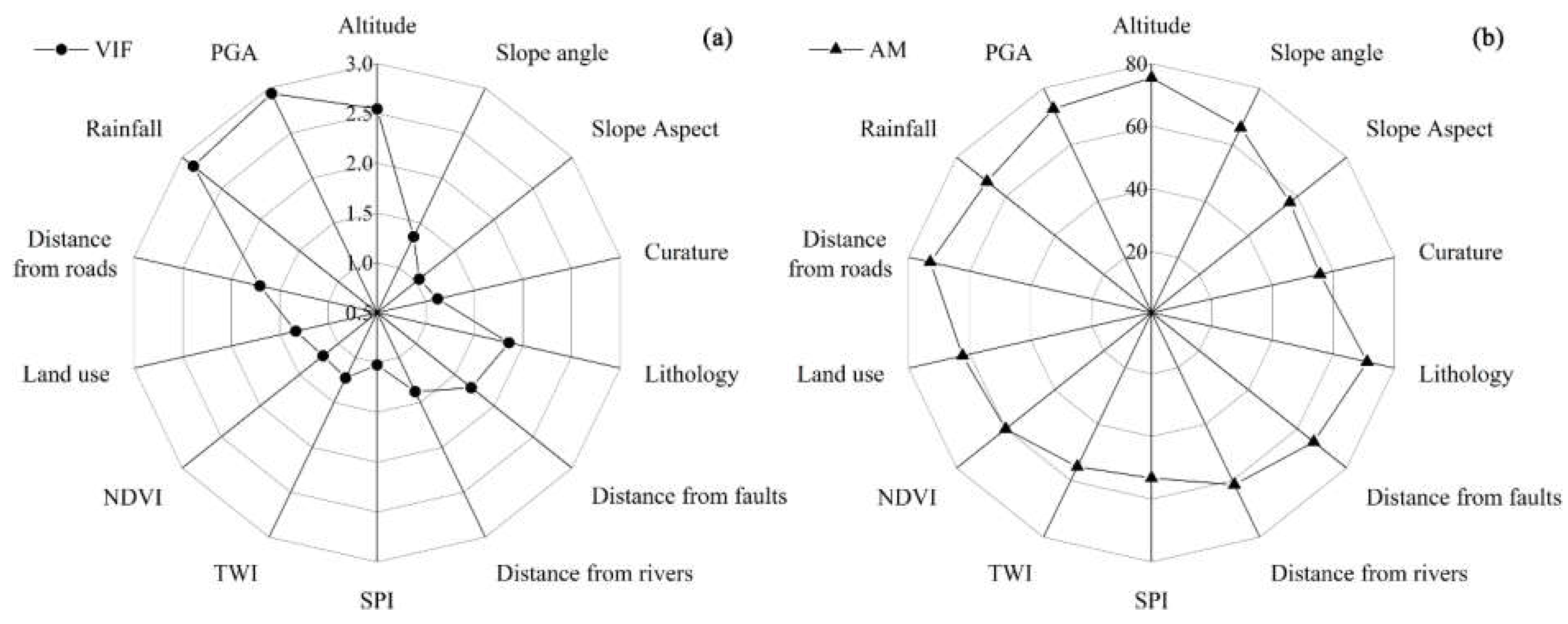
3.2. Feature Selection

The effectiveness of a landslide susceptibility assessment depends significantly on the quality and quantity of the utilized data, especially the variables that affect landslide occurrences in a given area [46]. In the present study, the variance inflation factor (VIF) and one rule (One-R) technique were employed to analyze the multicollinearity problem and predictive ability for the variables, respectively. Generally, a VIF of less than 5 indicates that the variables are independent [47]. The One-R technique can estimate and rank the importance of conditioning variables. For each variable, a rule is separately built in the training dataset, and the simple rule with the smallest error metric is selected for modeling [48]. Error metrics for each variable and each variable’s value are computed. The variables are then ranked based on the quality of the corresponding rules indicated by the average merit (AM) index [49]. Irrelevant or unimportant factors can be removed without much damage to information through feature selection [50].

3.3. Landslide Susceptibility Model

3.3.1. Bayesian Network (BN)

The BN algorithm provides a systematic method for describing uncertainty interdependencies among random variables based on graph theory and Bayes condition probability [20], which has great potential for natural hazard assessment. BN generally consists of a directed acyclic graph for the qualitative component and a set of Bayesian conditional probabilities for the quantitative dataset, which are described in [51,52]. Landslide susceptibility assessment can be regarded as a way to solve the multivariable joint probability distribution function. The BN can use the chain rule and the conditional independence relationship between landslide variables to decompose the joint distribution into the products of several less complex probability distributions [53], which can be expressed as follows:

$$P(X_1,\dots ,X_n)={\displaystyle \prod _{i=1}^{n}P(X_i|\pi (X_i))}$$

(2)

where P(X₁, …, X_n) represents the joint distribution of n variables; π(X_i) is the parent nodes of X_i; and P(X_i|π(X_i)) is the conditional probability distribution of X_i given π(X_i).

3.3.2. Decision Table (DTable)

A DTable is a scheme-specific learning algorithm that uses a table structure to refine the description of complex logic. The algorithm is usually performed using a default rule mapping to the majority class [32]. It has two parts: (i) a schema containing a set of features in the table and (ii) a body composed of labeled instances from the space defined by the features in the schema [54]. In this study, the best-first search was used to obtain good attribute combinations.

3.3.3. Radial Basis Function Network (RBFN)

An RBFN is a type of receptive-field neural network for function approximation [55]. The RBFN has a feedforward structure that comprises three layers (input layer, hidden layer, and output layer) (Figure 4). The input layer connects the inputs from the dataset, which includes 14 landslide-related variables. The output layer predicts a landslide or non-landslide. The hidden layer contains a specialized radial basis function that serves as an activation function, which is usually represented by the Gaussian function. More detailed introductions about the RBFN are provided in [31,56]. The RBFN is beneficial as it can easily solve the high-dimensional space nonlinearity problem through a set of linear combinations of radial basis functions and has the ability to be quickly trained [57]. Therefore, it has been successfully applied to solve many complex problems related to the environment, such as flood and landslide susceptibility modeling [55].

3.3.4. Stochastic Gradient Descent (SGD)

The SGD is one of the most popular ML algorithms for model optimization; it is generally applicable to support discriminative learning of linear classifiers under convex loss functions, such as neural networks, SVMs, and LR [58]. SGD is an improved algorithm that is based on gradient descent. This algorithm is regarded as a stochastic approximation of the gradient descent optimization as it uses an approximation gradient instead of an actual gradient by randomly subsampling the whole training dataset [59]. The algorithm is popular because of its high efficiency and easy implementation for datasets with redundant samples. However, SGD is rarely applied in landslide susceptibility analyses, which need to be widely explored. In this study, LR is used as a loss function in modeling.

3.4. Model Evaluation and Comparison

To evaluate the performance of the four models, a set of statistical indices, including the positive predictive rate (PPR), negative predictive rate (NPR), sensitivity, specificity, accuracy (ACC), F-measure (F₁), and Cohen’s kappa (k) coefficient, were utilized for the training and validation datasets. These methods are broadly adopted to define the performance of the spatial models and are explained in detail in [31]. The higher the statistical indices are, the better the model performance is, which is a perfect model with a value of 1 [19]. They can be calculated using the following formulas [18,25,50]:

$$\mathrm{PPR}=\frac{\mathrm{TP}}{\mathrm{TP}+\mathrm{FP}}$$

(3)

$$\mathrm{NPR}=\frac{\mathrm{TN}}{\mathrm{TN}+\mathrm{FN}}$$

(4)

$$\mathrm{Sensitivity}=\frac{\mathrm{TP}}{\mathrm{TP}+\mathrm{FN}}$$

(5)

$$\mathrm{Specificity}=\frac{\mathrm{TN}}{\mathrm{FP}+\mathrm{TN}}$$

(6)

$$\mathrm{ACC}=\frac{\mathrm{TP}+\mathrm{TN}}{\mathrm{TP}+\mathrm{FP}+\mathrm{TN}+\mathrm{PN}}$$

(7)

$${\mathrm{F}}_1=\frac{2\times \mathrm{Sensitivity}\times \mathrm{PPR}}{\mathrm{Sensitivity}+\mathrm{PPR}}$$

(8)

$$k=\frac{ACC-AC{C}_{\exp }}{1-AC{C}_{\exp }}$$

(9)

$$AC{C}_{\exp }=\frac{\left(\mathrm{TP}+\mathrm{FN}\right)\left(\mathrm{TP}+\mathrm{FP}\right)+\left(\mathrm{FP}+\mathrm{TN}\right)\left(\mathrm{TN}+\mathrm{FN}\right)}{{\left(\mathrm{TP}+\mathrm{TN}+\mathrm{FP}+\mathrm{FN}\right)}^2}$$

(10)

where TP (true positive) and TN (true negative) are the numbers of pixels that are correctly classified as landslides. FP (false positive) and FN (false negative) are the numbers of pixels that are incorrectly classified. ACC_exp is the expected accuracy.

Apart from the statistical indices, the ROC curve that plots “sensitivity” as the y-axis against “1-specificity” as the x-axis and the corresponding AUCs were employed for evaluation [25]. The AUC value ranges from 0.5 to 1.0, and a higher value indicates better model performance. The predictive capability given the AUC value could be quantified as follows: excellent (0.9–1), very good (0.8–0.9), good (0.7–0.8), average (0.6–0.7), and poor (0.5–0.6) [42].

4. Results and Analysis

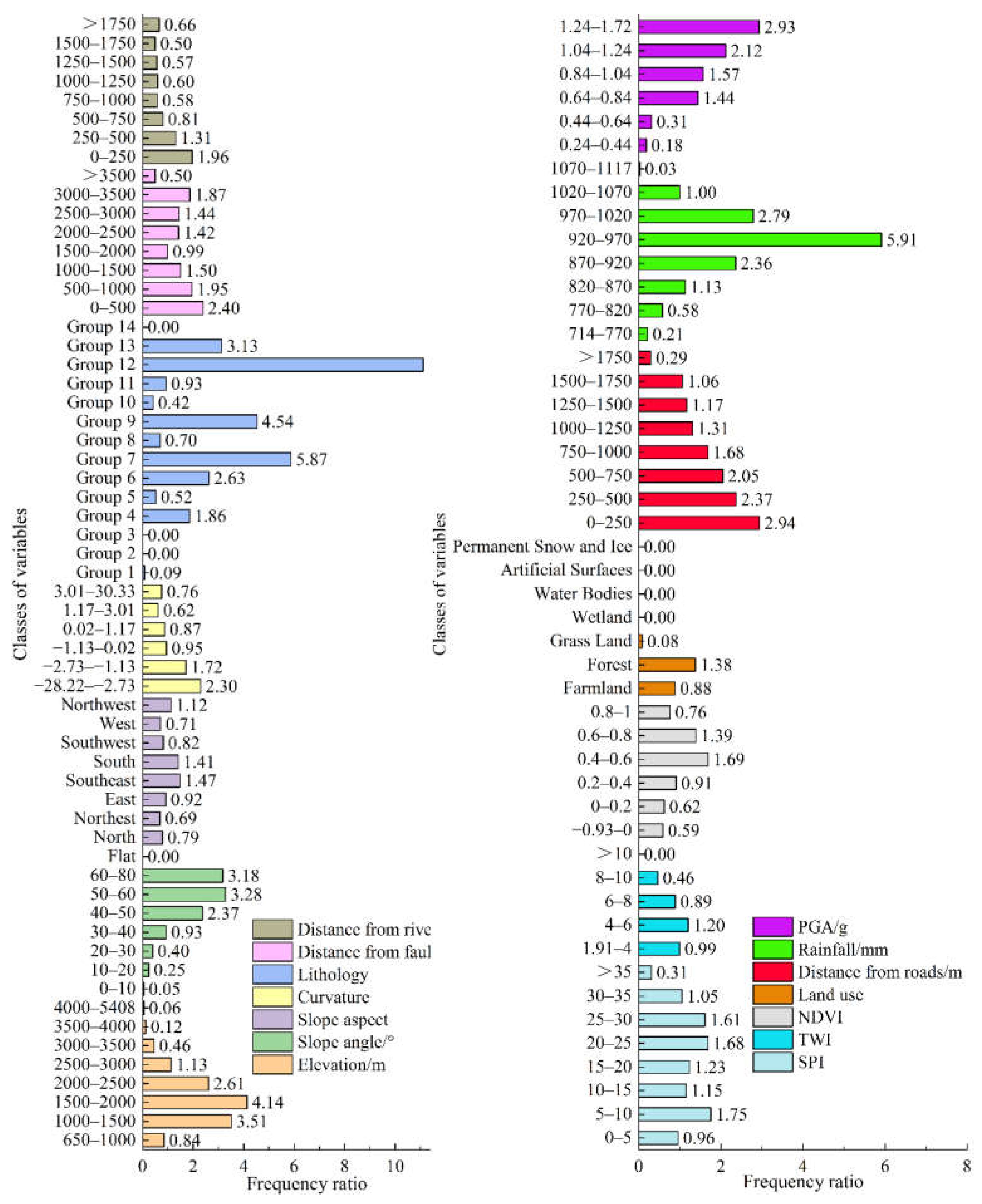
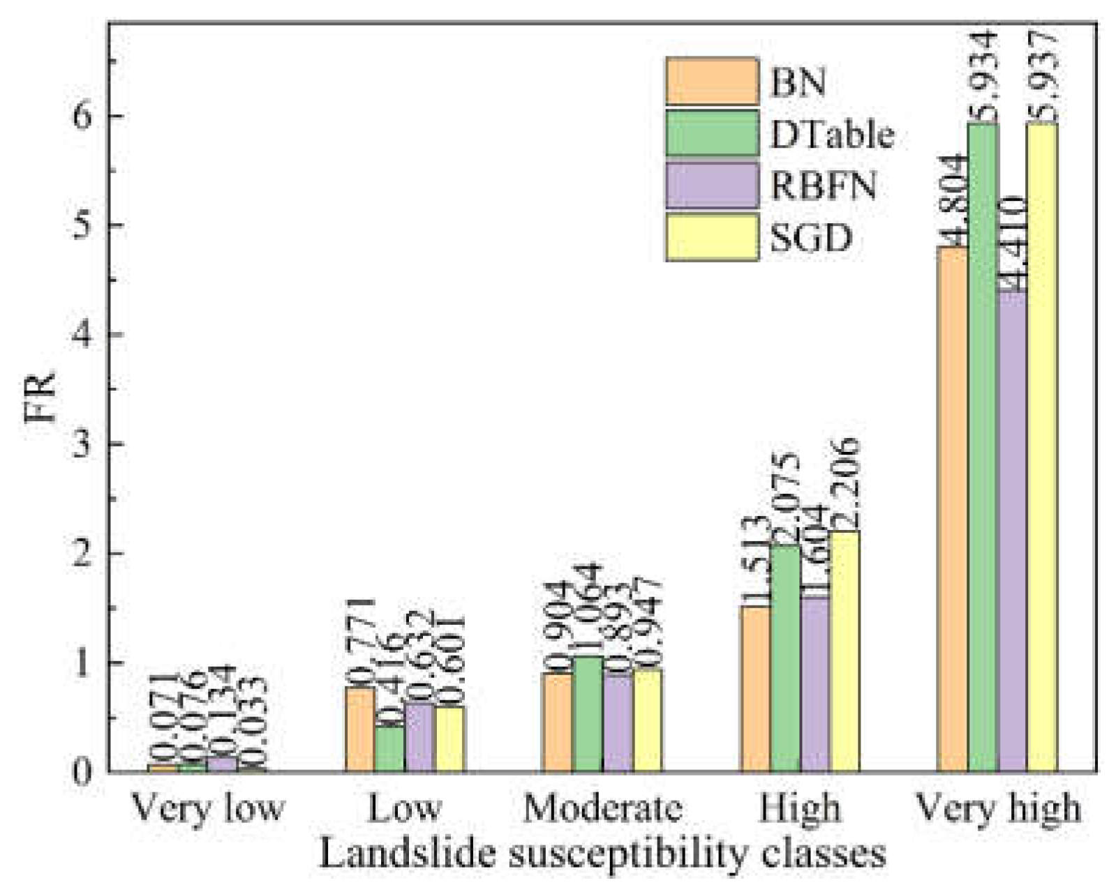
4.1. FR Analysis

4.1.1. Topographic Variables

The mathematical calculation of the FR value for all variables is presented in Figure 5. For the altitude, the subclasses of 1000–1500 m, 1500–2000 m, 2000–2500 m, and 2500–3000 have FR values > 1, meaning landslides are prone to occur in these zones. In this study, the areas with an altitude < 3000 m are mainly distributed in the piedmont basin and on both banks of the river. In these areas, most agricultural activities and engineering constructions may affect the stability of hillslopes. However, the FR value in the range of 650–1000 m is less than 1 as most of these areas are located around Dujiangyan city with a plain area of the Sichuan Basin where landslides do not occur. For the slope angle, the subclasses of 40–50°, 50–60°, and 60–80° possess FR values larger than 1, indicating that steep terrain is conducive to the occurrence of landslides. Generally, the FR value basically shows an increasing trend with an increase in the slope angle. In the field survey, we discovered that many rockfalls occurred in steep rock slopes on both sides of the river valley. For the slope aspect, hillslopes with dip directions of southeast (FR = 1.47), south (FR = 1.41), and northwest (FR = 1.12) exhibit a higher probability of causing landslides. In the case of curvature, the class (−28.22)–(−2.73) has the highest FR values (FR = 2.30), followed by the class (−2.73)–(−1.13) (FR = 1.72), indicating that hillslopes with concave shapes usually have a higher probability of landslide occurrence.

4.1.2. Geological Variables

For lithology, six classes with FR values > 1 can be observed, involving group 4 (FR = 1.86), group 6 (FR = 2.63), group 7 (FR = 5.87), group 9 (FR = 4.54), group 12 (FR = 11.11), and group 13 (FR = 3.13). All these lithological units are sedimentary and magmatic rocks, which are distributed from Dujiangyan city to Gengda town. For the distance from faults, intervals of 0–500 m have the highest FR value (FR = 2.40), indicating that landslides are prone to occur in these areas. Three main active faults, namely, PGF, BYF, and MWF, cross the study area, where the Wenchuan Ms 8.0 earthquake is related to BYF.

4.1.3. Hydrological Variables

Overall, FR values have a negative correlation with the distance from rivers. Concretely, classes of 0–250 m and 250–500 m have the highest FR values of 1.96 and 1.32, respectively. Regarding the SPI, except for the classes of 0–5 and >35, which have FR values < 1, the other classes display a positive influence on landslide occurrence. Classes 5–10 are the most prone to hillslope failure, with FR = 1.75. For the TWI, the relationship between the five classes and landslide occurrence shows a distinction among classes. Classes 4–6 are the most prone to sliding (FR = 1.20), whereas the other classes are relatively unlikely to slide.

4.1.4. Environmental Variables

With respect to the NDVI, the maximum FR value (FR = 1.69) belongs to the class of 0.4–0.6, followed by the class of 0.6–0.8 (FR = 1.39), suggesting susceptibility to landslides. Concerning land use, most landslides occurred in the forest area (FR = 1.38), followed by farmland (FR = 0.88) and grass land (FR = 0.08). For the distance from roads, the correlation with the occurrence of landslides decreases with an increase in distance from roads. FR values > 1 in the classes with distances in the ranges of 0−250 m, 250−500 m, 500−750 m, 750−1000 m, 1000−1250 m, 1250−1500 m, and 1500−1750 m indicate that within a certain range (<1750 m), road construction has a positive impact on the occurrence of landslides. In terms of rainfall, the probability of landslides increases with an increase in rainfall, reaching a maximum in the class of 920−970 mm (FR = 5.91) and then decreasing. This result is mainly because rainfall is concentrated in the piedmont basin, where landslides rarely occur. Judging from the PGA results, the FR values gradually increase as the PGA values rise. The PGA class of 1.24–1.72 g occupied the highest value for FR (2.93). Within a certain range, the positive effects of PGA on slope stabilities gradually increase with an increase in PGA.

4.2. Feature Selection Analysis

The VIF and AM index of 14 variables were calculated with the training dataset, and the results are shown in Figure 6. All VIF values are less than 5, which indicates that no variables have significant multicollinearity (Figure 6a). Moreover, altitude, distance from roads, and PGA, with AM values of 75.42, 72.89, and 72.71, respectively, are the most important variables and have the highest predictive capabilities for landslide modeling (Figure 6b). From the feature selection results, we determined that all fourteen variables had significance in landslide incidence (AM > 0); thus, all variables were utilized for landslide susceptibility modeling in this study.

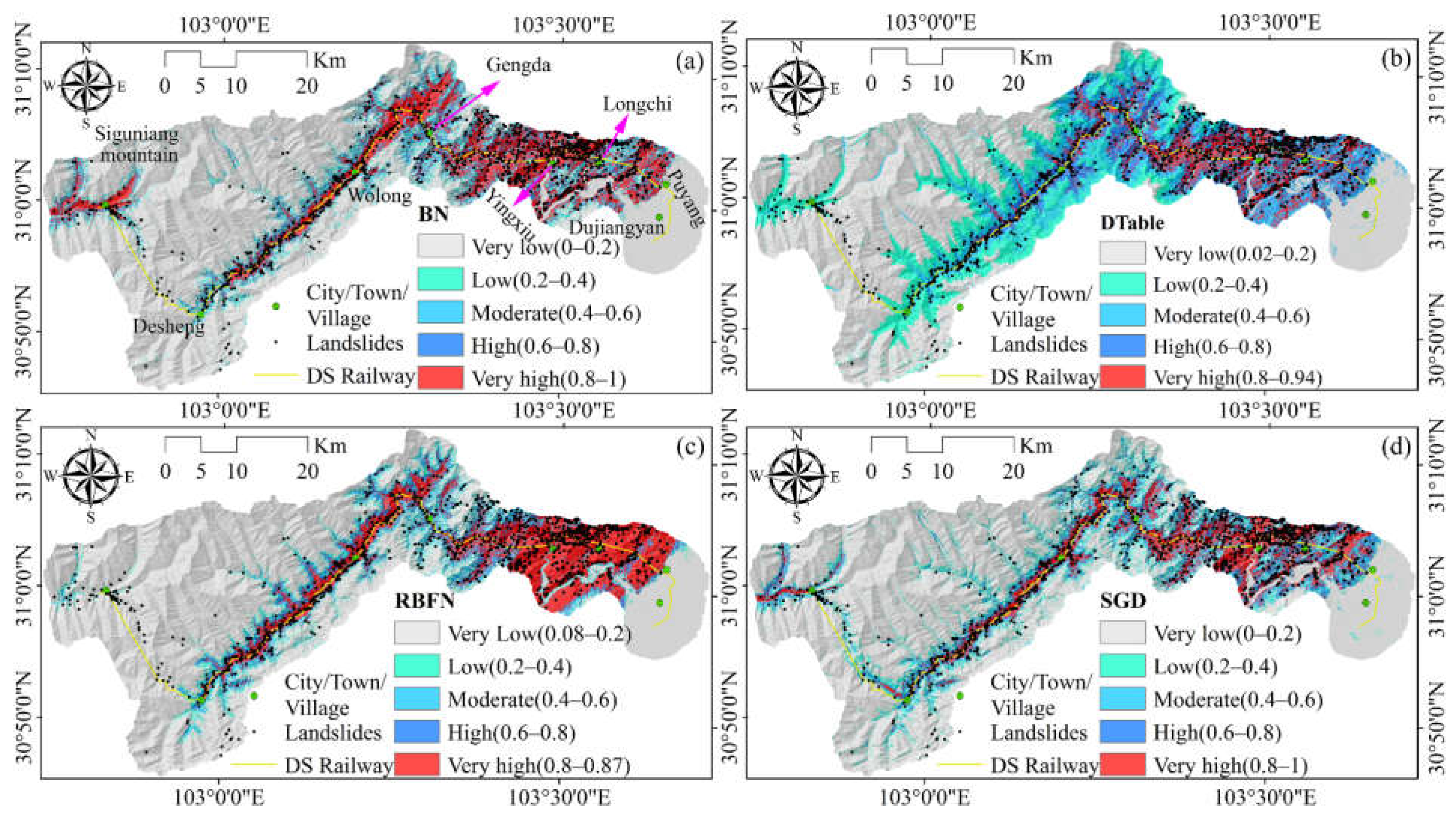
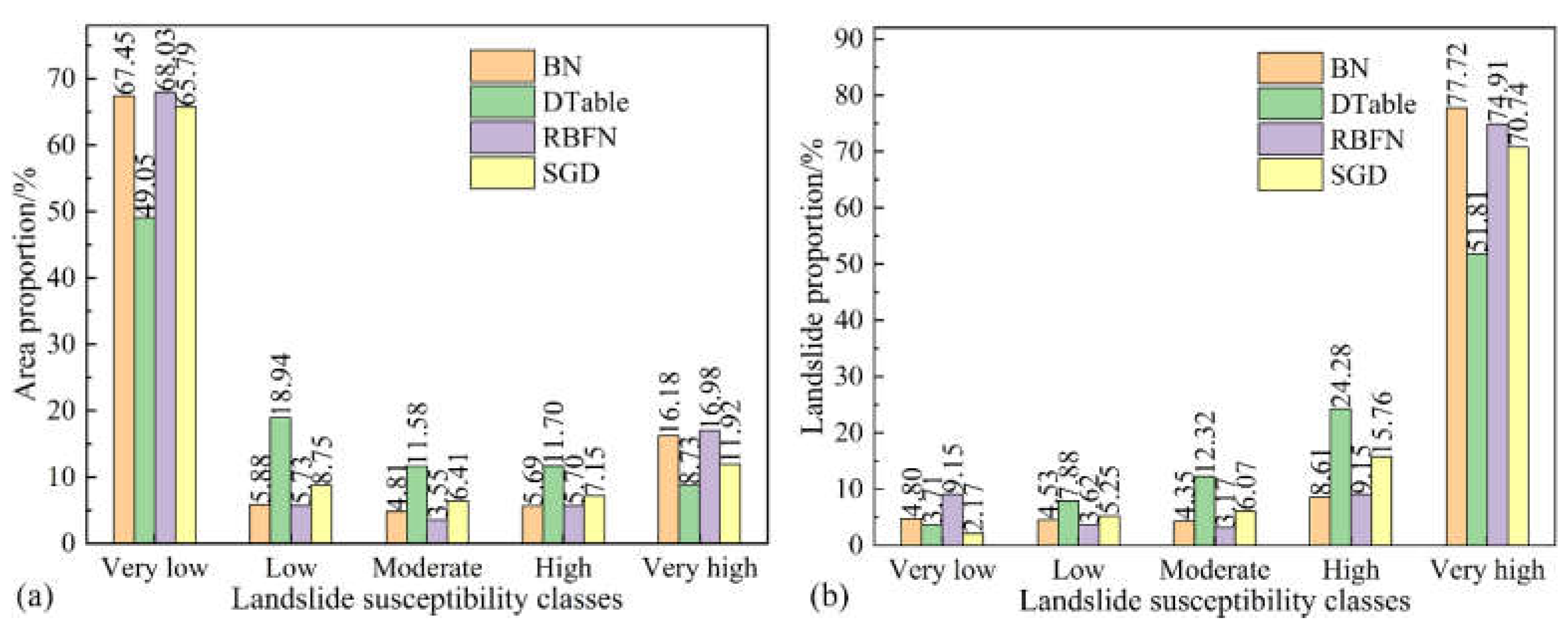
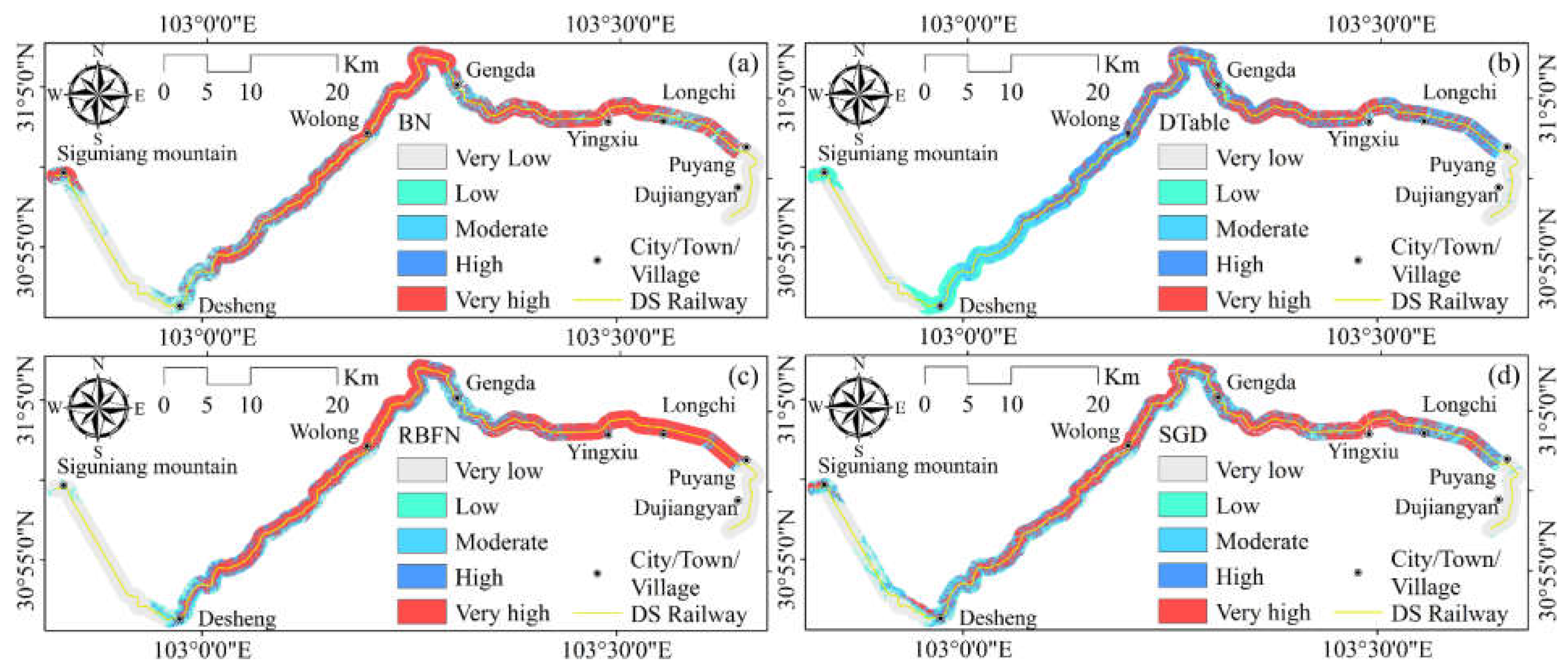
4.3. Application of the Models

LSMs were produced for the four models using the 14 variables, and the results are presented in Figure 7. More precisely, the landslide susceptibility index (LSI) for each pixel of the study area was calculated using the trained models in WEKA software. These LSI values were then demarcated into five classes by means of the equal interval classification method in the GIS environment, correspondingly, very low (0–0.2), low (0.2–0.4), moderate (0.4–0.6), high (0.6–0.8), and very high (0.8–1). Note that, the most prevailing natural breaks method was not selected to divide landslide susceptibility classes in this study, as the ranges and distributions of LSI values produced by various models usually vary. There is no comparability among the LSMs obtained by the natural breaks method, which is a defect that cannot be disregarded [23]. Therefore, for correct comparison of the LSMs generated by the BN, DTable, RBFN, and SGD models, an equal interval of 0.2 was used to identify landslide susceptibility levels. For more clarification, the area and landslide proportions in each landslide susceptibility class are shown in Figure 8.

In this case, the results show that the LSI values derived from the BN model range from 0 to 1 (Figure 7a). We found that the very low landslide susceptibility class covered the largest areas of the whole study area (67.45%), followed by the very high (16.18%), low (5.88%), high (5.69%), and moderate (4.81%) classes (Figure 8a). For the DTable model, the LSI values are between 0.02 and 0.94 (Figure 7b). The area classified as very low was the largest (49.05%), followed by low (18.94%), high (11.70%), moderate (11.58%), and very high (8.73%) (Figure 8a). Regarding the RBFN model, the LSI values range from 0.08 to 0.87 (Figure 7c). According to Figure 8a, the very low class has the largest coverage area (68.03%), followed by the very high (16.98%), low (5.73%), high (5.70%), and moderate (3.55%) classes. In the case of the SGD model, the LSI values range from 0 to 1 (Figure 7d). Here, 65.79% of the study area has very low landslide susceptibility, while the differences in area percentages among very high (11.92%), low (8.75%), high (7.15%), and moderate (6.41%) levels are relatively slight (Figure 8a). Notably, 49.05−68.03% of the whole domain belongs to very low susceptibility zones produced by the four models, which are mainly located in high mountains above 3500 m, the water bodies/reservoir, and the piedmont plain. However, the very high and high susceptibility zones are mainly distributed near rivers, roads, steep slopes, and magmatic rock-covered areas in the study area.

In Figure 8b, 86.32%, 76.09%, 84.06%, and 86.50% of all landslides fall in the high- and very high-susceptibility zones produced by the BN, DTable, RBFN, and GSD models, respectively. However, for the very low and low susceptibility classes, the BN, DTable, RBFN, and GSD models involve 9.33%, 11.59%, 12.77%, and 7.43% landslide points, respectively. As a result, compared with the BN, DTable, and RBFN models, the map obtained by SGD may show more precision.

In addition, the FR of landslide occurrence in different landslide susceptibility classes was calculated to evaluate the reliability of these maps (Figure 9). The results show that the greatest percentage of landslide occurrence belongs to the very high-susceptibility class, followed by the high, moderate, low, and very low classes. This finding demonstrates that the applied models can effectively determine different landslide susceptibility classes in the study area [60]. Based on the FR value in the very high-susceptibility level, the highest value of 5.937 is obtained for the SGD model, which indicates that the map generated by the SGD model is better than that of other models (BN, DTable, and RBFN).

LSMs of the 1 km buffer zone along the proposed DS railway were extracted to exhibit the possible impact of landslides within a specific range along the railway (Figure 10). The buffer zone with an area of 245.87 km² involved 468 landslides, accounting for 42.39% of all landslides. According to the area proportion of landslide susceptibility classes within the buffer zone (Figure 11a), we found that 47.11−58.32% of buffer zones are located in zones with high- and very high-susceptibility to landslides, while the very low zone only occupies 24.45−31.35% of the buffer zone. Obviously, the high- and very high-susceptibility zones mainly spread along the railway from Puyang town to Desheng village.

Based on the landslide inventory map in the buffer regions, the largest landslide points (92.52%) match the high and very high classes identified by the SGD model, followed by the RBFN, BN, and DTable models (Figure 11b). However, approximately 8.97% of landslides are distributed in low and very low landslide susceptibility zones calculated by the DTable model, which is larger than that of the RBFN (7.70%), BN (5.34%), and SGD models (3.42%). Therefore, the SGD model is more accurate than the BN, RBFN, and DTable models.

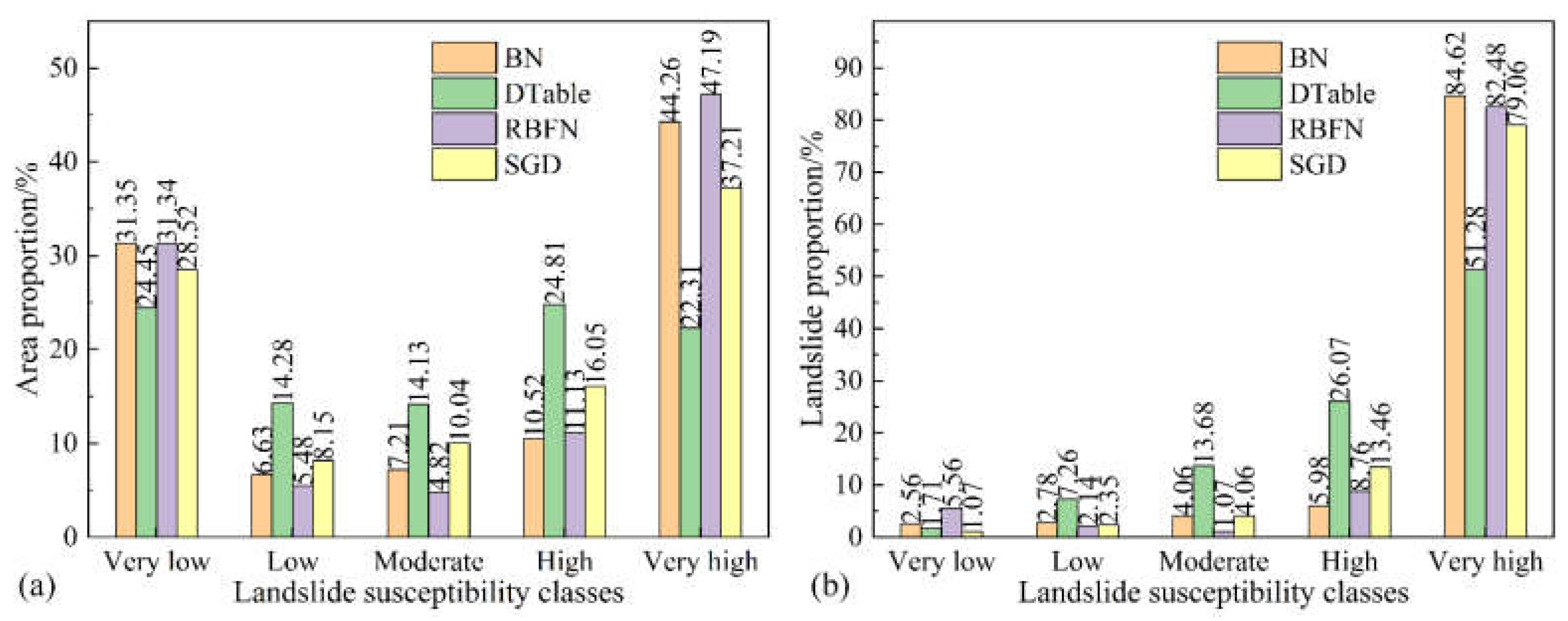
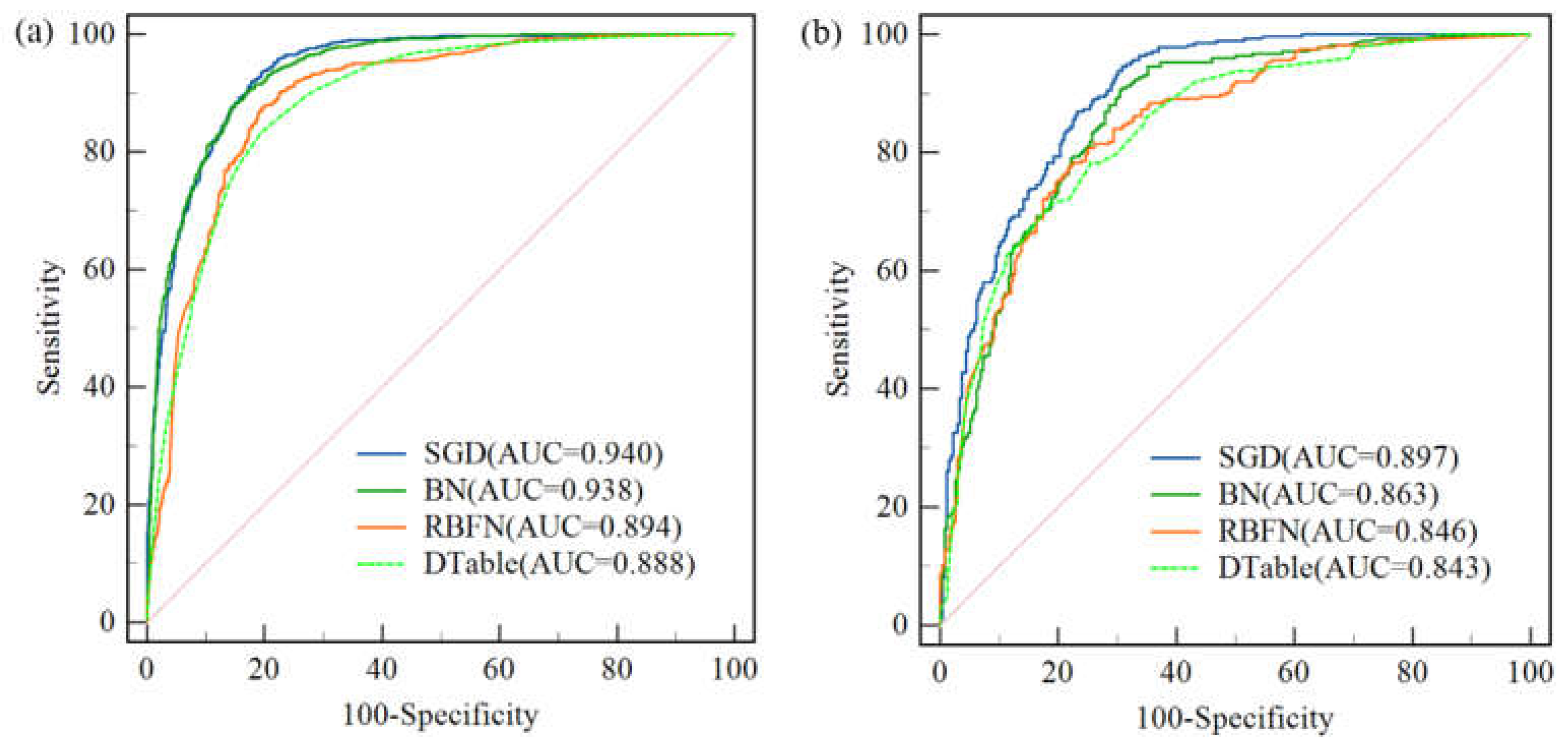
4.4. Performance and Comparison of Models

The performance of the applied models was assessed and compared using statistical indices (

Table 3. Statistical index results of different models.

Parameters	Training Dataset				Validation Dataset
	SGD	BN	RBFN	DTable	SGD	BN	RBFN	DTable
True positive	758	751	726	688	232	231	219	216
True negative	682	679	664	668	215	204	208	206
False positive	146	149	164	160	61	72	68	70
False negative	70	77	102	140	44	45	57	60
PPR/%	83.85	83.44	81.57	81.13	79.18	76.24	76.31	75.52
NPR/%	90.69	89.81	86.68	82.67	83.01	81.93	78.49	77.44
Sensitivity/%	91.55	90.70	87.68	83.09	84.06	83.70	79.35	78.26
Specificity/%	82.37	82.00	80.19	80.67	77.90	73.91	75.36	74.64
ACC/%	86.96	86.35	83.94	81.88	80.98	78.80	77.36	76.45
F1	0.88	0.87	0.85	0.82	0.82	0.80	0.78	0.77
k	0.74	0.73	0.68	0.64	0.62	0.58	0.55	0.53

). For the performance of the landslide training dataset, the SGD model had the highest performance accuracy compared to the BN, RBFN, and DTable models, with higher values of PPR (83.85%), NPR (90.69%), sensitivity (91.55%), specificity (82.37%), ACC (86.96%), F₁ (0.88) and k (0.74).

Very similar results can be obtained for the testing prediction accuracy using the landslide validation dataset. The statistical indices demonstrate that the SGD model (PPR = 79.18%, NPR = 83.01%, sensitivity = 84.06%, specificity = 77.90%, ACC = 80.98%, F₁ = 0.82, and k = 0.62) performed best, followed by BN (PPR = 76.24%, NPR = 81.93%, sensitivity = 83.70%, specificity = 73.91%, ACC = 78.80%, F₁ = 0.80, and k = 0.58), RBFN (PPR = 76.31%, NPR = 78.49%, sensitivity = 79.35%, specificity = 75.36%, ACC = 77.36%, F₁ = 0.78, and k = 0.55), and DTable (PPR = 75.52%, NPR = 77.44%, sensitivity = 78.26%, specificity = 74.64%, ACC = 76.45%, F₁ = 0.77, and k = 0.53).

The overall performance of the landslide models using the AUC of the ROC curve based on both the training and validation datasets is illustrated in Figure 12. For the training dataset, it can be observed that the SGD (AUC = 0.940) and BN (AUC = 0.938) models presented excellent performance (AUC > 0.9), while RBFN (AUC = 0.894) and DTable (AUC = 0.888) achieved very good performance (AUC = 0.8–0.9) in this study. As a result, the SGD model outperformed the BN, RBFN, and DTable models. With the validation dataset, the results confirmed that the four prediction models presented very good performances (AUC > 0.8). The SGD achieved the highest performance with an AUC value of 0.897, followed by the BN (AUC = 0.863), RBFN (AUC = 0.846), and DTable (AUC = 0.843) models.

5. Discussion

In mountain areas, climate change, land-use changes, and engineering construction increases may exacerbate the risk of landslides. However, the prediction and assessment of landslides are still lacking for specific linear engineering in the southwest mountainous areas of China. Therefore, in the present study, we implement a detailed comparison to evaluate the performances of four advanced ML models (BN, DTable, RBFN, and SGD) in identifying landslide-prone areas along the DS railway.

Before training these models, this study used multicollinearity analysis and the One-R technique to select reasonable variables. The results obtained by the multiple collinearity analysis indicated that the 14 variables were independent. Moreover, the AM values of all the variables are larger than 0, which can reveal the main geo-environmental features and landslide triggering mechanism in this region. Specifically, the impact of altitude on landslides is much higher than that of other variables in this region (AM = 75.42). This observation is consistent with several previous studies [42,61]. Human activities are intensive within a certain elevation range. More high-susceptibility areas are located in the range of 1000–3000 m, which is also consistent with our statistics on the actual altitude at which landslides are more prone to occur. In addition, distance from roads is an important variable affecting the probability of landslides (AM = 72.89). In mountainous areas, the road can destroy the original balance of the slope, resulting in slope instability (Figure 2b). Combined with the LSMs analysis, the high and very high landslide-prone areas are mainly clustered near the roads. Therefore, in the process of railway construction, we should avoid slope cutting and strengthen the support of existing slope cutting. PGA, another extrinsic variable, also has a significant effect on the occurrence of landslides (AM = 72.71). According to the FR analysis, the greater the PGA is, the greater the possibility of landslides in the study area. It was observed that most landslides occurred in Yingxiu and Longchi towns, with PGAs greater than 1.24 g. These analyses indicate that the occurrence of landslides is closely related to the surrounding geo-environmental conditions.

Based on the statistical indices and AUC, the SGD model performed best with corresponding assessment metrics of AUC = 0.940, ACC = 86.96%, F₁ = 0.88 and k = 0.74 for the training dataset and AUC = 0.897, ACC = 80.98%, F₁ = 0.82 and k = 0.62 for the validation dataset. The reason is related to the applicability and reliability of this algorithm in processing large-scale landslide data. This algorithm can recover good solutions to minimize training errors and generalize well in complex and nonconvex models [62]. This algorithm has the advantages of simplicity, low computational cost, fast convergence, and reliable effect [63,64]. Several scholars have already exploited the SGD model to address large-scale problems and obtain accurate findings [65,66]. However, the BN, DTable, and RBFN models also performed better, as the AUC value was greater than 0.8 on both the training and validation datasets. The advantage of the BN is that it can handle missing data even with small sample sizes [29]. The DTable is easy to understand and can accurately classify instances in discrete spaces [54]. The RBFN has the properties of unique global approximation, linear relationship of output weights in the network structure, good classification ability, and fast training speed [67]. Furthermore, there is minimal discrepancy between the prediction ability of the training dataset and that of the validation dataset, which demonstrates that the four algorithms do not have an overfitting problem [39]. Therefore, all four models can achieve good outcomes and can be used to obtain highly reliable and practical LSMs along the DS railway.

The choice of the study area boundary is very important for landslide susceptibility assessment, and multiple relevant boundaries such as administrative boundaries, line buffer zones, and watershed boundaries have been applied [43,61,68]. Among these boundaries, line buffer zones were widely utilized to divide the research area for linear engineering. However, there is no uniform standard for the boundary range of linear engineering. Few studies address the maximum limit range of disaster impact on both sides of line engineering [68]. This study’s object is the landslide susceptibility assessment along the DS railway. The landforms crossed by the DS railway, including the piedmont basin, mountains, and alpine-gorge, are quite complex. Therefore, we applied a combination of line buffer zones and watershed boundaries to determine the study area. In the piedmont basin, landslides rarely occurred, so we use a buffer zone of approximately 5 km as the research boundary. Many landslides occurred from Puyang to Yingxiu, and the research boundaries were divided according to the distribution of historical landslides and the possible influence range of landslides. In the alpine-gorge area from Yingxiu to Siguniang mountain towns, some high landslides have a large influence scope. Therefore, we delineated the study area boundary according to the watershed boundaries, which is a fairly stable method for railway construction. We also focused on the susceptibility of landslides in the 1 km buffer zone along the DS railway (Figure 10), as the landslide susceptibility near the railway is the most noteworthy area in engineering research, which can provide a basis for railway route selection, and necessary intervention measures can be taken in advance. In addition, a 1 km buffer zone is extracted for analysis to compare the performance of the four models at a specific scale. The results of the landslide proportion within a 1 km buffer zone along the DS railway also show that the SGD model is the most accurate, followed by the BN, RBFN, and DTable models (Figure 11).

From the LSMs produced by the four models, 8.73−16.98% of the whole domain is very prone to landslides, which are mainly distributed near rivers and roads. The areas with very low landslide susceptibility are mainly located in high mountains above 3500 m and piedmont plains. Overall, the DS railway from Puyang town to Dengsheng village traverses areas with high and very high susceptibility to landslides. Significantly, there are also some differences in the spatial distribution of each class for the four models. For instance, Siguniang Mountain town is in a very high-susceptibility area based on the LSMs obtained by the BN and SGD models, but the DTable and RBFN models reveal that the town is in a moderate or very low susceptibility area (Figure 7). According to the spatial location of landslides in Siguniang Mountain town (Figure 7), the BN and SGD models are more accurate. Based on the LSMs, railways will be threatened by landslides in the process of construction and operation. At present, the proposed railway from Puyang town to Dengsheng village is suggested to traverse mountain tunnels, and local sections outside the mountain can be connected by roads or bridges. For some tunnel entrances and exits located in high-risk areas, we suggest strengthening the detailed investigation on tunnel hillslopes. If necessary, the position of the tunnel entrance can be changed, or effective engineering support measures can be taken. For low susceptibility zones, potential geohazards still need to be investigated and monitored. In addition, the investigation of high-hidden landslide hazards and the stability analysis of high-steep slopes or cut slopes around the railway line are the focus of future research.

However, certain uncertainty and limitations should be noted. Landslide-related variables have diverse sources, and the spatial resolution of the variables (e.g., DEM, lithology, distance from faults, and NDVI) was not always consistent (Table 1), which is a major shortcoming of this study. Choosing a spatial resolution that is appropriate for all datasets is still a challenge. Among the 14 variables, both topographic and hydrological variables were extracted from a DEM with a spatial resolution of 30 m. Notably, lithology and faults were obtained by vectoring the 1:200,000 geological map, which has been applied in many studies of landslide susceptibility [23]. The position accuracy, attribute accuracy, and joint accuracy of these data meet the technical regulations and requirements and can provide enough spatial information. For the simplicity of data processing, we resampled all the thematic layers at a 30 m resolution. Due to the constraints of data, accurately defining the uncertainty induced by inconsistent spatial resolution is difficult [21]. However, we believe that our results are valuable for landslide susceptibility mapping. In addition, the obtained LSMs are not stationary and will change over time, as dynamic factors (such as rainfall, land use, distance from roads, and NDVI) will change the condition of landslide probability. Reichenbach, et al. [2] observed that landslide susceptibility changed in response to land-use changes from 1954 to 2009. Therefore, the validity period of susceptibility assessment is the direction of further research. Decision-makers should strengthen the monitoring of dynamic variables to reduce disasters.

6. Conclusions

Here, four advanced ML methods (BN, DTable, RBFN, and SGD) were selected to map landslide probabilities along the DS railway. The major findings of this study can be summarized as follows:

(1) Multicollinearity analysis was performed for 14 variables, and the One-R technique was used to estimate factor importance ranking. The 14 selected variables had no multicollinearity problems, and altitude, distance from roads, and PGA were more important to landslides in the study area.

(2) The precision of the models used in this research was validated using the AUC of ROC curves and statistical indices. The results show that all four ML models can reasonably and accurately predict landslide susceptibility. However, the SGD model achieved the highest prediction accuracy with the highest ACC value (80.98%), F₁ value (0.82), k (0.62), and AUC value (0.897), followed by the BN (ACC = 78.80%, F₁ = 0.80, k = 0.58, and AUC = 0.863), RBFN (ACC = 77.36%, F₁ = 0.78, k = 0.55, and AUC = 0.846), and DTable (ACC = 76.45%, F₁ = 0.77, k = 0.53, and AUC = 0.843) models.

(3) The produced susceptibility maps showed that more than one-fifth of the study area has high to very high susceptibility to landslides, which mainly spread along the railway from Puyang town to Desheng village. Therefore, in the project planning, construction, and operation stages, it is necessary to strengthen the investigation, monitoring, and prevention of landslide hazards in the above areas. The information obtained from LSMs could help planners develop warning systems and mitigation measures during the construction of the DS railway. Notably, the findings of the present study may also be beneficial to landslide risk mitigation and land-use planning of other line engineering construction projects in similar environmental settings.

References

1. Juliev, M.; Mergili, M.; Mondal, I.; Nurtaev, B.; Pulatov, A.; Hubl, J. Comparative analysis of statistical methods for landslide susceptibility mapping in the Bostanlik District, Uzbekistan. Sci. Total Environ. 2019, 653, 801–814. [Google Scholar] [CrossRef] [PubMed]
2. Reichenbach, P.; Busca, C.; Mondini, A.C.; Rossi, M. The Influence of Land Use Change on Landslide Susceptibility Zonation: The Briga Catchment Test Site (Messina, Italy). Environ. Manag. 2014, 54, 1372–1384. [Google Scholar] [CrossRef] [PubMed] [Green Version]
3. Guzzetti, F.; Peruccacci, S.; Rossi, M.; Stark, C.P. The rainfall intensity-duration control of shallow landslides and debris flows: An update. Landslides 2008, 5, 3–17. [Google Scholar] [CrossRef]
4. Zou, Q.; Jiang, H.; Cui, P.; Zhou, B.; Jiang, Y.; Qin, M.; Liu, Y.; Li, C. A new approach to assess landslide susceptibility based on slope failure mechanisms. Catena 2021, 204, 105388. [Google Scholar] [CrossRef]
5. Clark, M.K.; Schoenbohm, L.M.; Royden, L.H.; Whipple, K.X.; Burchfiel, B.C.; Zhang, X.; Tang, W.; Wang, E.; Chen, L. Surface uplift, tectonics, and erosion of eastern Tibet from large-scale drainage patterns. Tectonics 2004, 23, 1–20. [Google Scholar] [CrossRef] [Green Version]
6. Hetzel, R. Active faulting, mountain growth, and erosion at the margins of the Tibetan Plateau constrained by in situ-produced cosmogenic nuclides. Tectonophysics 2013, 582, 1–24. [Google Scholar] [CrossRef]
7. Wang, G.; Huang, R.; Lourenço, S.D.N.; Kamai, T. A large landslide triggered by the 2008 Wenchuan (M8.0) earthquake in Donghekou area: Phenomena and mechanisms. Eng. Geol. 2014, 182, 148–157. [Google Scholar] [CrossRef] [Green Version]
8. Huang, J.P.; Sun, C.W.; Wu, X.Y.; Ling, S.X.; Wang, S.; Deng, R. Stability assessment of tunnel slopes along the Dujiangyan City to Siguniang Mountain Railway, China. Bull. Eng. Geol. Environ. 2020, 79, 5309–5327. [Google Scholar] [CrossRef]
9. Wu, R.A.; Zhang, Y.S.; Guo, C.B.; Yang, Z.H.; Tang, J.; Su, F.R. Landslide susceptibility assessment in mountainous area: A case study of Sichuan-Tibet railway, China. Environ. Earth Sci. 2020, 79, 157. [Google Scholar] [CrossRef]
10. Quinn, P.E.; Hutchinson, D.J.; Diederichs, M.S.; Rowe, R.K. Regional-scale landslide susceptibility mapping using the weights of evidence method: An example applied to linear infrastructure. Can. Geotech. J. 2010, 47, 905–927. [Google Scholar] [CrossRef]
11. Ngo, P.T.T.; Panahi, M.; Khosravi, K.; Ghorbanzadeh, O.; Kariminejad, N.; Cerda, A.; Lee, S. Evaluation of deep learning algorithms for national scale landslide susceptibility mapping of Iran. Geosci. Front. 2021, 12, 505–519. [Google Scholar]
12. Brabb, E.E. Innovative approaches to landslide hazard mapping. In Proceedings of the Fourth International Symposium on Landslides, Canadian Geotechnical Society, Toronto, ON, Canada, 16–21 September 1984; pp. 307–324. [Google Scholar]
13. Reichenbach, P.; Rossi, M.; Malamud, B.D.; Mihir, M.; Guzzetti, F. A review of statistically-based landslide susceptibility models. Earth-Sci. Rev. 2018, 180, 60–91. [Google Scholar] [CrossRef]
14. Neuland, H. A prediction model of landslips. Catena 1976, 3, 215–230. [Google Scholar] [CrossRef]
15. Merghadi, A.; Yunus, A.P.; Dou, J.; Whiteley, J.; ThaiPham, B.; Bui, D.T.; Avtar, R.; Abderrahmane, B. Machine learning methods for landslide susceptibility studies: A comparative overview of algorithm performance. Earth-Sci. Rev. 2020, 207, 103225. [Google Scholar] [CrossRef]
16. Yilmaz, I. Landslide susceptibility mapping using frequency ratio, logistic regression, artificial neural networks and their comparison: A case study from Kat landslides (Tokat-Turkey). Comput. Geosci. 2009, 35, 1125–1138. [Google Scholar] [CrossRef]
17. Goetz, J.N.; Brenning, A.; Petschko, H.; Leopold, P. Evaluating machine learning and statistical prediction techniques for landslide susceptibility modeling. Comput. Geosci. 2015, 81, 1–11. [Google Scholar] [CrossRef]
18. Huang, F.M.; Cao, Z.S.; Guo, J.F.; Jiang, S.H.; Li, S.; Guo, Z.Z. Comparisons of heuristic, general statistical and machine learning models for landslide susceptibility prediction and mapping. Catena 2020, 191, 104580. [Google Scholar] [CrossRef]
19. Chen, W.; Zhang, S.; Li, R.W.; Shahabi, H. Performance evaluation of the GIS-based data mining techniques of best-first decision tree, random forest, and naive Bayes tree for landslide susceptibility modeling. Sci. Total Environ. 2018, 644, 1006–1018. [Google Scholar] [CrossRef] [PubMed]
20. Pham, B.T.; Pradhan, B.; Bui, D.T.; Prakash, I.; Dholakia, M.B. A comparative study of different machine learning methods for landslide susceptibility assessment: A case study of Uttarakhand area (India). Environ. Modell. Softw. 2016, 84, 240–250. [Google Scholar] [CrossRef]
21. Yi, Y.N.; Zhang, Z.J.; Zhang, W.C.; Jia, H.H.; Zhang, J.Q. Landslide susceptibility mapping using multiscale sampling strategy and convolutional neural network: A case study in Jiuzhaigou region. Catena 2020, 195, 104851. [Google Scholar] [CrossRef]
22. Youssef, A.M.; Pourghasemi, H.R.; Pourtaghi, Z.S.; Al-Katheeri, M.M. Landslide susceptibility mapping using random forest, boosted regression tree, classification and regression tree, and general linear models and comparison of their performance at Wadi Tayyah Basin, Asir Region, Saudi Arabia. Landslides 2016, 13, 839–856. [Google Scholar] [CrossRef]
23. Chen, W.W.; Zhang, S. GIS-based comparative study of Bayes network, Hoeffding tree and logistic model tree for landslide susceptibility modeling. Catena 2021, 203, 105344. [Google Scholar] [CrossRef]
24. Zhang, S.T.; Wang, F.F.; Duo, F.; Zhang, J.L. Research on the Majority Decision Algorithm based on WeChat sentiment classification. J. Intell. Fuzzy Syst. 2018, 35, 2975–2984. [Google Scholar] [CrossRef]
25. Bui, D.T.; Shahabi, H.; Omidvar, E.; Shirzadi, A.; Geertsema, M.; Clague, J.J.; Khosravi, K.; Pradhan, B.; Pham, B.T.; Chapi, K.; et al. Shallow Landslide Prediction Using a Novel Hybrid Functional Machine Learning Algorithm. Remote Sens. 2019, 11, 931. [Google Scholar]
26. Hong, H.Y.; Tsangaratos, P.; Ilia, I.; Loupasakis, C.; Wang, Y. Introducing a novel multi-layer perceptron network based on stochastic gradient descent optimized by a meta-heuristic algorithm for landslide susceptibility mapping. Sci. Total Environ. 2020, 742, 140549. [Google Scholar] [CrossRef] [PubMed]
27. Nhu, V.H.; Hoang, N.D.; Nguyen, H.; Ngo, P.T.T.; Bui, T.T.; Hoa, P.V.; Samui, P.; Bui, D.T. Effectiveness assessment of Keras based deep learning with different robust optimization algorithms for shallow landslide susceptibility mapping at tropical area. Catena 2020, 188, 104458. [Google Scholar] [CrossRef]
28. Wang, W.D.; He, Z.L.; Han, Z.; Li, Y.G.; Dou, J.; Huang, J.L. Mapping the susceptibility to landslides based on the deep belief network: A case study in Sichuan Province, China. Nat. Hazards 2020, 103, 3239–3261. [Google Scholar] [CrossRef]
29. Song, Y.Q.; Gong, J.H.; Gao, S.; Wang, D.C.; Cui, T.J.; Li, Y.; Wei, B.Q. Susceptibility assessment of earthquake-induced landslides using Bayesian network: A case study in Beichuan, China. Comput. Geosci. 2012, 42, 189–199. [Google Scholar] [CrossRef]
30. Lee, S.; Lee, M.J.; Jung, H.S.; Lee, S. Landslide susceptibility mapping using Naive Bayes and Bayesian network models in Umyeonsan, Korea. Geocarto Int. 2020, 35, 1665–1679. [Google Scholar] [CrossRef]
31. Pham, B.T.; Trung, N.T.; Qi, C.C.; Phong, T.V.; Dou, J.; Ho, L.S.; Le, H.V.; Prakash, I. Coupling RBF neural network with ensemble learning techniques for landslide susceptibility mapping. Catena 2020, 195, 104805. [Google Scholar] [CrossRef]
32. Pham, B.T.; Vu, V.D.; Costache, R.; Phong, T.V.; Ngo, T.Q.; Tran, T.H.; Nguyen, H.D.; Amiri, M.; Tan, M.T.; Trinh, P.T.; et al. Landslide susceptibility mapping using state-of-the-art machine learning ensembles. Geocarto Int. 2021, 36, 1–26. [Google Scholar] [CrossRef]
33. Deng, B.; Liu, S.G.; Jansa, L.; Cao, J.X.; Cheng, Y.; Li, Z.W.; Liu, S. Sedimentary record of Late Triassic transpressional tectonics of the Longmenshan thrust belt, SW China. J. Asian Earth Sci. 2012, 48, 43–55. [Google Scholar] [CrossRef]
34. Li, Y.; Cao, S.; Zhou, R.; Densmore, A.L.; Ellis, M.A. Late Cenozoic Minjiang Incision Rate and Its Constraint on the Uplift of the Eastern Margin of the Tibetan Plateau. Acta Geol. Sin. 2005, 79, 28–37. [Google Scholar]
35. Hungr, O.; Leroueil, S.; Picarelli, L. The Varnes classification of landslide types, an update. Landslides 2014, 11, 167–194. [Google Scholar] [CrossRef]
36. Chen, W.; Chen, X.; Peng, J.B.; Panahi, M.; Lee, S. Landslide susceptibility modeling based on ANFIS with teaching-learning-based optimization and Satin bowerbird optimizer. Geosci. Front. 2021, 12, 93–107. [Google Scholar] [CrossRef]
37. Youssef, A.M.; Pradhan, B.; Jebur, M.N.; El-Harbi, H.M. Landslide susceptibility mapping using ensemble bivariate and multivariate statistical models in Fayfa area, Saudi Arabia. Environ. Earth Sci. 2015, 73, 3745–3761. [Google Scholar] [CrossRef]
38. Shao, X.Y.; Ma, S.Y.; Xu, C.; Zhang, P.F.; Wen, B.Y.; Tian, Y.Y.; Zhou, Q.; Cui, Y.L. Planet Image-Based Inventorying and Machine Learning-Based Susceptibility Mapping for the Landslides Triggered by the 2018 Mw6.6 Tomakomai, Japan Earthquake. Remote Sens. 2019, 11, 978. [Google Scholar] [CrossRef] [Green Version]
39. Rahman, M.; Chen, N.S.; Elbeltagi, A.; Islam, M.M.; Alam, M.; Pourghasemi, H.R.; Tao, W.; Zhang, J.; Tian, S.F.; Faiz, H.; et al. Application of stacking hybrid machine learning algorithms in delineating multi-type flooding in Bangladesh. J. Environ. Manag. 2021, 295, 113086. [Google Scholar] [CrossRef]
40. Zhao, Y.; Wang, R.; Jiang, Y.J.; Liu, H.J.; Wei, Z.L. GIS-based logistic regression for rainfall-induced landslide susceptibility mapping under different grid sizes in Yueqing, Southeastern China. Eng. Geol. 2019, 259, 105147. [Google Scholar] [CrossRef]
41. Kavzoglu, T.; Sahin, E.K.; Colkesen, I. Selecting optimal conditioning factors in shallow translational landslide susceptibility mapping using genetic algorithm. Eng. Geol. 2015, 192, 101–112. [Google Scholar] [CrossRef]
42. Chen, W.; Xie, X.; Wang, J.; Pradhan, B.; Hong, H.; Bui, D.T.; Duan, Z.; Ma, J. A comparative study of logistic model tree, random forest, and classification and regression tree models for spatial prediction of landslide susceptibility. Catena 2017, 151, 147–160. [Google Scholar] [CrossRef] [Green Version]
43. Tsangaratos, P.; Ilia, I. Comparison of a logistic regression and Naive Bayes classifier in landslide susceptibility assessments: The influence of models complexity and training dataset size. Catena 2016, 145, 164–179. [Google Scholar] [CrossRef]
44. Wang, Y.; Fang, Z.C.; Hong, H.Y.; Costache, R.; Tang, X.Z. Flood susceptibility mapping by integrating frequency ratio and index of entropy with multilayer perceptron and classification and regression tree. J. Environ. Manag. 2021, 289, 112449. [Google Scholar] [CrossRef]
45. Lee, S.; Pradhan, B. Landslide hazard mapping at Selangor, Malaysia using frequency ratio and logistic regression models. Landslides 2007, 4, 33–41. [Google Scholar] [CrossRef]
46. Shahabi, H.; Shirzadi, A.; Ronoud, S.; Asadi, S.; Pham, B.T.; Mansouripour, F.; Geertsema, M.; Clague, J.J.; Bui, D.T. Flash flood susceptibility mapping using a novel deep learning model based on deep belief network, back propagation and genetic algorithm. Geosci. Front. 2021, 12, 101100. [Google Scholar] [CrossRef]
47. Chen, X.; Chen, W. GIS-based landslide susceptibility assessment using optimized hybrid machine learning methods. Catena 2021, 196, 104833. [Google Scholar] [CrossRef]
48. Holte, R.C. Very Simple Classification Rules Perform Well on Most Commonly Used Datasets. Mach. Learn. 1993, 11, 63–91. [Google Scholar] [CrossRef]
49. Pes, B. Ensemble feature selection for high-dimensional data: A stability analysis across multiple domains. Neural Comput. Appl. 2020, 32, 5951–5973. [Google Scholar] [CrossRef] [Green Version]
50. Luu, C.; Pham, B.T.; Phong, T.V.; Costache, R.; Nguyen, H.D.; Amiri, M.; Bui, Q.D.; Nguyen, L.T.; Le, H.V.; Prakash, I.; et al. GIS-based ensemble computational models for flood susceptibility prediction in the Quang Binh Province, Vietnam. J. Hydrol. 2021, 599, 126500. [Google Scholar] [CrossRef]
51. Pearl, J. Chapter 3—Markov and Bayesian Networks: Two Graphical Representations of Probabilistic Knowledge. In Probabilistic Reasoning in Intelligent Systems; Pearl, J., Ed.; Morgan Kaufmann: San Francisco, CA, USA, 1988; pp. 77–141. [Google Scholar]
52. Wu, Z.N.; Shen, Y.X.; Wang, H.L.; Wu, M.M. Assessing urban flood disaster risk using Bayesian network model and GIS applications. Geomat. Nat. Haz. Risk 2019, 10, 2163–2184. [Google Scholar] [CrossRef] [Green Version]
53. Lu, Q.W.; Zhong, P.A.; Xu, B.; Zhu, F.L.; Ma, Y.F.; Wang, H.; Xu, S.Y. Risk analysis for reservoir flood control operation considering two- dimensional uncertainties based on Bayesian network. J. Hydrol. 2020, 589, 125353. [Google Scholar] [CrossRef]
54. Kohavi, R. The power of decision tables. In Proceedings of the Machine Learning: ECML-95, Berlin/Heidelberg, Germany, 25–27 April 1995; pp. 174–189. [Google Scholar]
55. He, Q.F.; Shahabi, H.; Shirzadi, A.; Li, S.J.; Chen, W.; Wang, N.Q.; Chai, H.C.; Bian, H.Y.; Ma, J.Q.; Chen, Y.T.; et al. Landslide spatial modelling using novel bivariate statistical based Naive Bayes, RBF Classifier, and RBF Network machine learning algorithms. Sci. Total Environ. 2019, 663, 1–15. [Google Scholar] [CrossRef] [PubMed]
56. Moody, J.; Darken, C.J. Fast Learning in Networks of Locally-Tuned Processing Units. Neural Comput. 1989, 1, 281–294. [Google Scholar] [CrossRef]
57. Chang, F.J.; Chen, Y.C. Estuary water-stage forecasting by using radial basis function neural network. J. Hydrol. 2003, 270, 158–166. [Google Scholar] [CrossRef]
58. El Bilali, A.; Taleb, A.; Nafii, A.; Alabjah, B.; Mazigh, N. Prediction of sodium adsorption ratio and chloride concentration in a coastal aquifer under seawater intrusion using machine learning models. Environ. Technol. Inno. 2021, 23, 101641. [Google Scholar] [CrossRef]
59. Le, H.V.; Hoang, D.A.; Tran, C.T.; Nguyen, P.Q.; Tran, V.H.T.; Hoang, N.D.; Amiri, M.; Ngo, T.P.T.; Nhu, H.V.; Hoang, T.V.; et al. A new approach of deep neural computing for spatial prediction of wildfire danger at tropical climate areas. Ecol. Inform. 2021, 63, 101300. [Google Scholar] [CrossRef]
60. Pham, B.T.; Phong, T.V.; Trung, N.T.; Parial, K.; Singh, S.K.; Ly, H.B.; Nguyen, K.T.; Ho, L.S.; Le, H.V.; Prakash, I. Ensemble modeling of landslide susceptibility using random subspace learner and different decision tree classifiers. Geocarto Int. 2020, 36, 1–23. [Google Scholar] [CrossRef]
61. Xie, W.; Li, X.S.; Jian, W.B.; Yang, Y.; Liu, H.W.; Robledo, L.F.; Nie, W. A Novel Hybrid Method for Landslide Susceptibility Mapping-Based GeoDetector and Machine Learning Cluster: A Case of Xiaojin County, China. Isprs Int. J. Geo-Inf. 2021, 10, 93. [Google Scholar] [CrossRef]
62. Lei, Y.W.; Tang, K. Learning Rates for Stochastic Gradient Descent with Nonconvex Objectives. IEEE T. Pattern Anal. 2021, 43, 4505–4511. [Google Scholar] [CrossRef] [PubMed]
63. Tang, M.Q.; Ren, C.J.; Xin, Y.L. Efficient Resource Allocation Algorithm for Underwater Wireless Sensor Networks Based on Improved Stochastic Gradient Descent Method. Ad Hoc Sens. Wirel. Netw. 2021, 49, 207–222. [Google Scholar]
64. Lei, Y.W.; Hu, T.; Tang, K. Generalization Performance of Multi-pass Stochastic Gradient Descent with Convex Loss Functions. J. Mach. Learn. Res. 2021, 22, 25–41. [Google Scholar]
65. Barani, F.; Savadi, A.; Yazdi, H.S. Convergence behavior of diffusion stochastic gradient descent algorithm. Signal Process. 2021, 183, 108014. [Google Scholar] [CrossRef]
66. Lyu, X.C.; Ren, C.S.; Ni, W.; Tian, H.; Liu, R.P.; Tao, X.F. Distributed Online Learning of Cooperative Caching in Edge Cloud. IEEE T. Mobile Comput. 2021, 20, 2550–2562. [Google Scholar] [CrossRef]
67. Kim, E.H.; Ko, J.H.; Oh, S.K.; Seo, K. Design of meteorological pattern classification system based on FCM-based radial basis function neural networks using meteorological radar data. Soft Comput. 2019, 23, 1857–1872. [Google Scholar] [CrossRef]
68. Zhao, F.M.; Meng, X.M.; Zhang, Y.; Chen, G.; Su, X.J.; Yue, D.X. Landslide Susceptibility Mapping of Karakorum Highway Combined with the Application of SBAS-InSAR Technology. Sensors 2019, 19, 2685. [Google Scholar] [CrossRef] [PubMed] [Green Version]
Figure 1. Location of the study area. (a) General map of China; (b) Location of the study area; (c) Landslide inventory map; (d) Topographic cross-section of D–D′ with different reliefs of approximately 3040 m. PGF: Pengxian-Guanxian faults, BYF: Beichuan-Yingxiu faults, MWF: Maoxian-Wenchuan faults.
Land 11 00436 g001
Figure 2. Photos showing landslides in the study region: (a) deep-seated rockslide triggered by the Wenchuan earthquake; (b) shallow rockslide triggered by road construction; (c) rockfall induced by joint cutting; and (d) rockfall caused by the Wenchuan earthquake.
Land 11 00436 g002
Figure 3. Landslide-related variables. (a) altitude, (b) slope angle, (c) slope aspect, (d) curvature, (e) lithology, (f) distance from faults, (g) distance from rivers, (h) SPI, (i) TWI, (j) NDVI, (k) land use, (l) distance from roads, (m) rainfall, and (n) PGA.
Land 11 00436 g003aLand 11 00436 g003b
Figure 4. Flowchart of the proposed methodology.
Land 11 00436 g004
Figure 5. FR of the landslides occurring in each class of variables.
Land 11 00436 g005
Figure 6. The VIF (a) and AM index (b) of the conditioning variables in the study area.
Land 11 00436 g006
Figure 7. LSMs for the study area produced by the (a) BN model, (b) DTable model, (c) RBFN model, and (d) SGD model.
Land 11 00436 g007
Figure 8. Quantitative analysis of the LSMs. (a) Area proportion of susceptibility classes. (b) Landslide proportion in each susceptibility class.
Land 11 00436 g008
Figure 9. Frequency ratio of landslides within susceptibility classes.
Land 11 00436 g009
Figure 10. LSMs for the railway 1 km buffer zone produced by the (a) BN model, (b) DTable model, (c) RBFN model, and (d) SGD model.
Land 11 00436 g010
Figure 11. Quantitative analysis of the landslide susceptibility maps within a 1 km buffer zone along the DS railway. (a) Area proportion of susceptibility classes. (b) Landslide proportion in each susceptibility class.
Land 11 00436 g011
Figure 12. ROC curve and AUC for four models: (a) training dataset and (b) validation dataset.
Land 11 00436 g012