Article

Understanding the Intensity of Land-Use and Land-Cover Changes in the Context of Postcolonial and Socialist Transformation in Kaesong, North Korea

1
Department of Geography, Graduate School of Korea University, 145 Anam-ro, Seongbuk-gu, Seoul 02841, Republic of Korea
2
Department of Geography Education, College of Education, Korea University, 145 Anam-ro, Seongbuk-gu, Seoul 02841, Republic of Korea
3
Institute of Future Land, Korea University, 145 Anam-ro, Seongbuk-gu, Seoul 02841, Republic of Korea
4
Department of Ecology & Environmental Sciences, Faculty of Science, Palacký University Olomouc, Šlechtitelů 27, 78371 Olomouc, Czech Republic
5
Graduate School of International Agricultural Technology, Seoul National University, 1447 Pyeongchangdaero, Daehwa, Pyeongchang 25354, Gangwon, Republic of Korea
6
Center for International Agricultural Development, Institutes of Green Bio Science and Technology, Seoul National University, 1447 Pyeongchangdaero, Daehwa, Pyeongchang 25354, Gangwon, Republic of Korea
7
Leibniz Institute of Ecological Urban and Regional Development, Weberplatz 1, 01217 Dresden, Germany
*
Author to whom correspondence should be addressed.
Land 2022, 11(3), 357; https://doi.org/10.3390/land11030357
Submission received: 13 January 2022 / Revised: 8 February 2022 / Accepted: 18 February 2022 / Published: 28 February 2022
(This article belongs to the Section Landscape Archaeology)

Abstract

:
This study examines the land-use and land-cover changes (LUCCs) in Kaesong, a North Korean city, and the area adjacent to the Korean Demilitarized Zone (DMZ). An intensity analysis—a framework decomposing LUCCs into interval, category, and transition levels—is applied to the land-cover maps of 1916, 1951, and 2015 to understand the importance of the historical period and associated land regimes (imperialism and socialism) in shaping LUCCs. The five land-cover classes—Built, Agriculture, Forest, Water, and Others—were analyzed among the two historical periods from Imperial Japan’s colonization (1910–1945) and the South–North division since the Korean War (1953–present). The results show that, at the interval level, the colonial period LUCCs were more intensive than the division period. However, >50% of the study area underwent changes during each period. At the category level, river channel modifications were the most intensive, followed by deforestation. In terms of transition, consistent intensity trends from Others to Built and Agriculture were observed across both land regimes. In conclusion, the LUCCs were more intensive under Japanese imperialism than the North Korean socialist regime, but the economic and geographic factors were not substantially affected by such land regimes. These underlying forces may be more significant fundamental drivers of LUCCs than land regimes themselves.

1. Introduction

Unlike in Europe, centralized socialist regimes are almost uniquely present in East Asia, often shaping their urban landscapes as they can determine the underlying political and socioeconomic forces driving land-use and land-cover changes (LUCCs) [1,2,3]. Urban landscapes are important because not only do they host the majority of the global population, their transformations are fundamental to the sustainability and resilience of societies [4,5,6]. Among Asian urban areas under centralized socialist regimes, LUCCs in cities and border regions of mainland China and Vietnam have been studied extensively via remote sensing data [7,8,9,10,11,12,13,14,15]. However, much less is known about LUCCs in North Korea (i.e., Democratic People’s Republic of Korea) or in areas along the inner border of South and North Korea [16,17,18,19,20,21].
The war between South and North Korea is technically ongoing, with this tension exemplified across the Korean Demilitarized Zone (DMZ). The DMZ represents the buffer zone delineated along the inner border between South and North Korea (i.e., the military demarcation line (MDL)), and both sides must withdraw 2 km from the MDL. Although land change in the DMZ has been previously studied, few researchers have focused on the nearby metropolitan areas that are likely to substantially affect the DMZ’s landscape [18,19,20,21].
Studies analyzing LUCCs of the DMZ regions are limited for various reasons. Land change research based primarily on remote sensing data typically lacks a historical context, as the dependency on satellite imagery restricts analyses prior to the 1970s [18,22]. The Korean Peninsula has undergone dynamic historical events, including colonization by Imperial Japan (1910–1945), the Korean War (1950–1953), and the South–North division since the Armistice Agreement (1953–present), all of which notably predate remote sensing data. Historical geographers and historians working on the DMZ rarely provide maps of LUCCs, as they typically lack the methodological toolsets for quantitatively capturing these spatial processes [23,24]. Thus, few Korean case studies have applied geographic information systems (GIS) and remote sensing techniques to analyze how, and to what degree, historical events have affected regional LUCC and shaped the landscape.
Accordingly, this study contributes to the understanding of land changes across different historical periods in the Korean Peninsula by investigating: (1) Which period over the previous century saw the most dynamic LUCC (fast vs. slow)? (2) Which land category went through the most intensive change (active vs. dormant)? (3) Which land transition was the most dominant (targeted vs. avoided)? The merit of applying an intensity analysis framework [25] to this case study is such that the analysis provides objective criteria to define which land change is “fast”, “active”, and “targeted”, compared to “slow”, “dormant”, and “avoided”, respectively. As mentioned, performing an intensity analysis for Kaesong, an area with an active and vibrant history, enables the quantification of LUCCs associated with the three separate historical events, defining two distinct periods, in a systematic manner. Specifically, we investigated the following research questions:
  • Considering the colonization by Imperial Japan and the South–North division, which of the two historical periods underwent more dynamic LUCCs?
  • Which land category went through the most intensive changes in the study area?
  • Were there any land transitions that clearly showed patterns of targeting or avoidance, regardless of historical period?

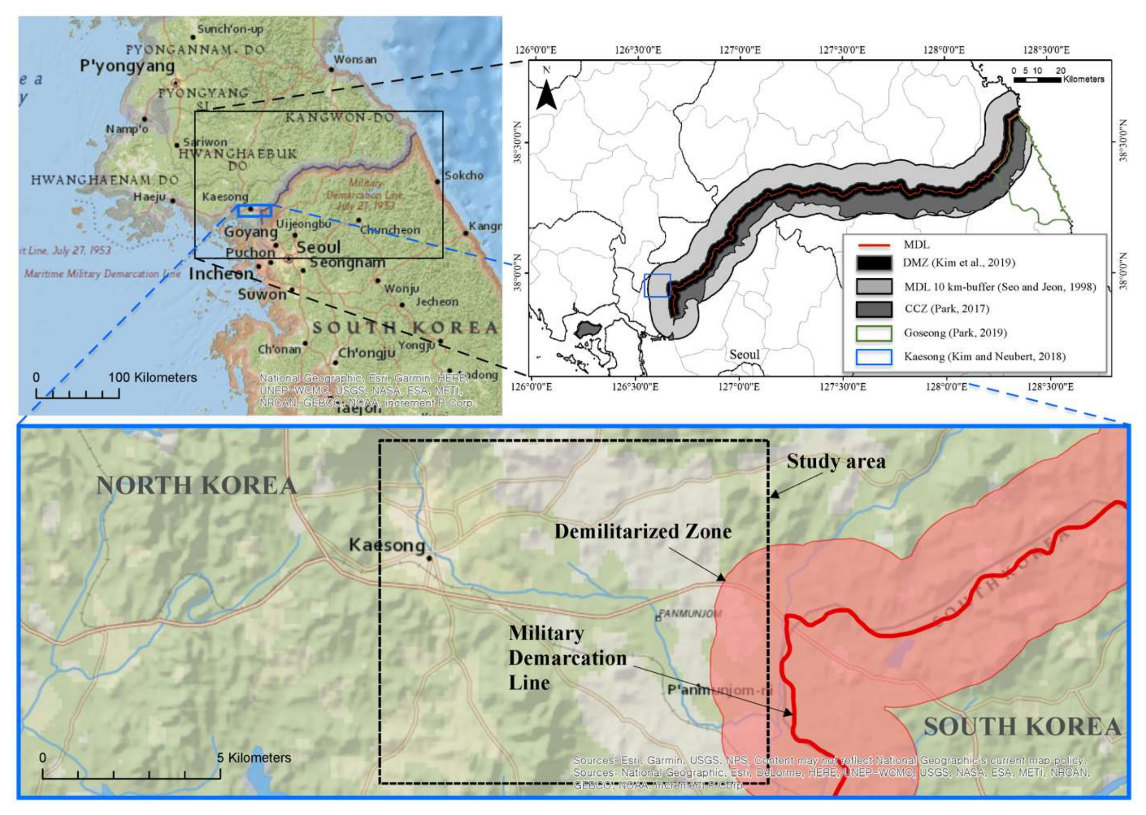
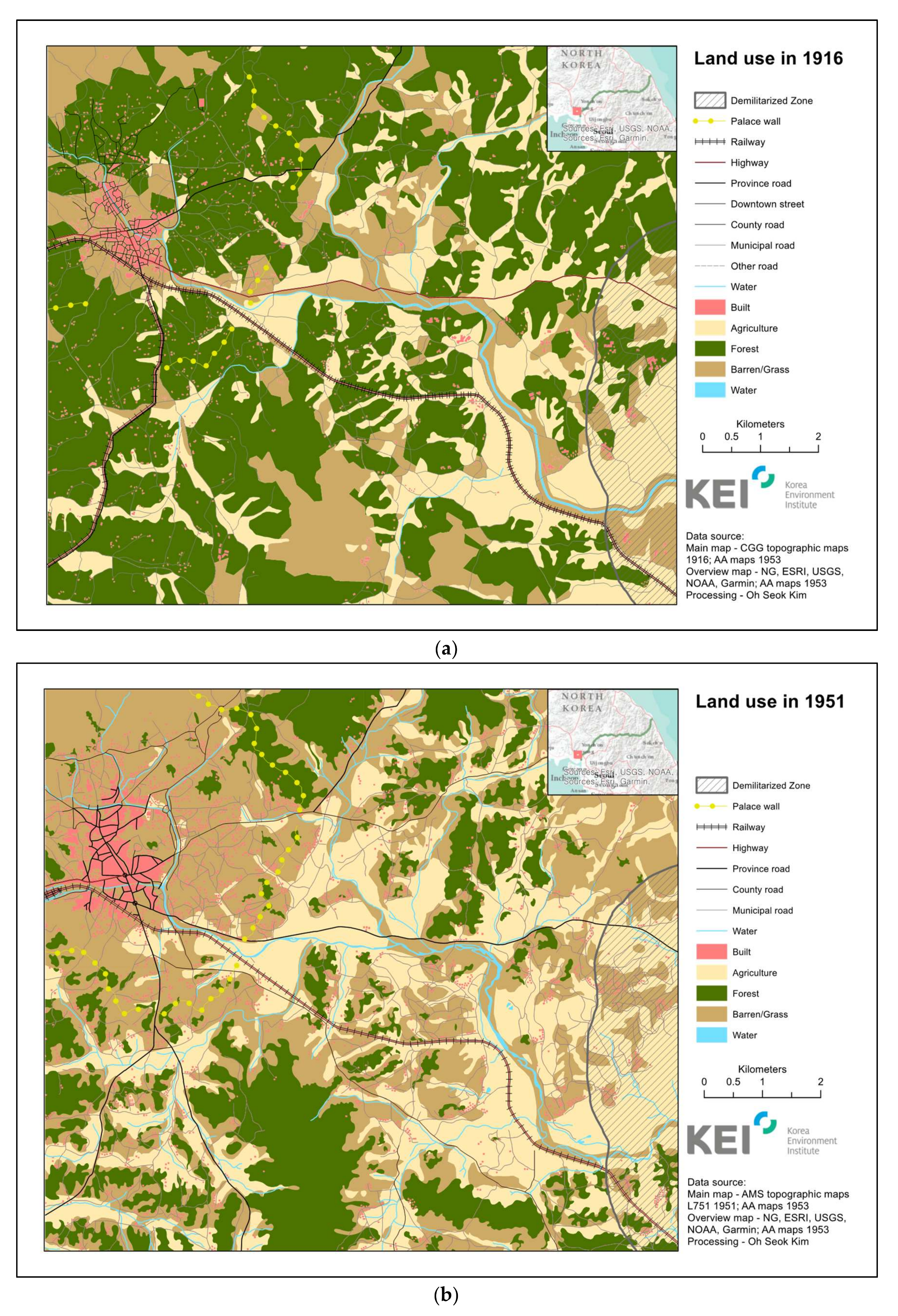
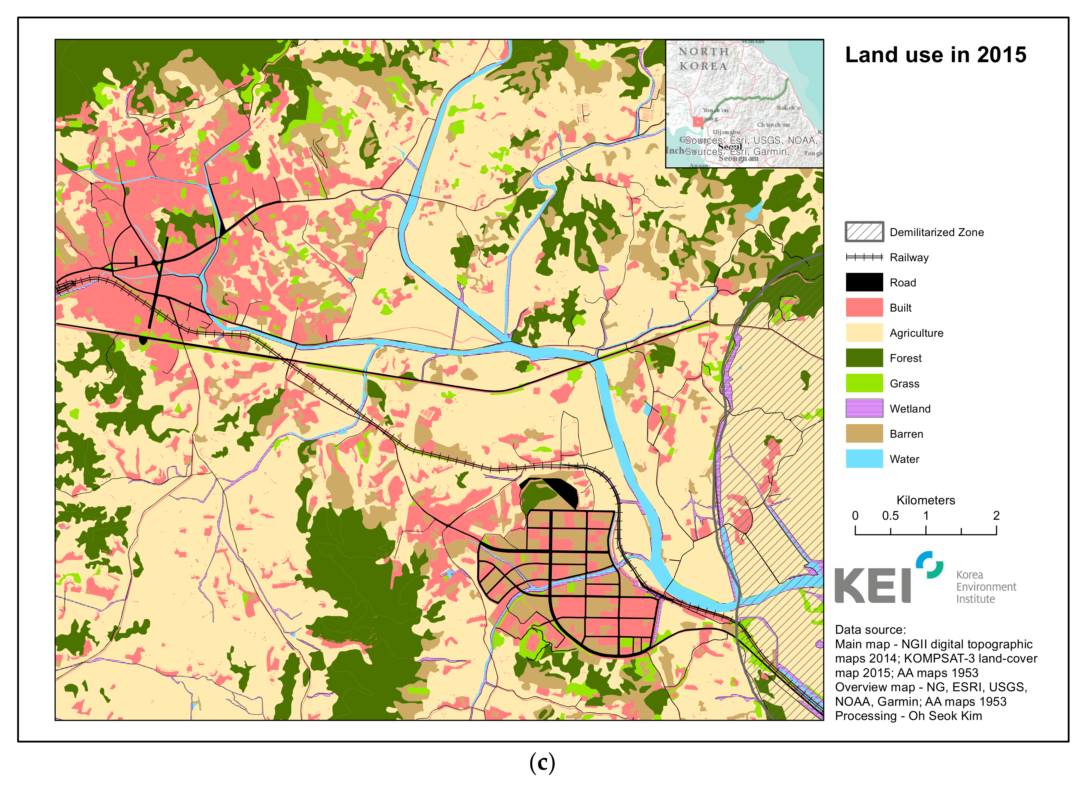
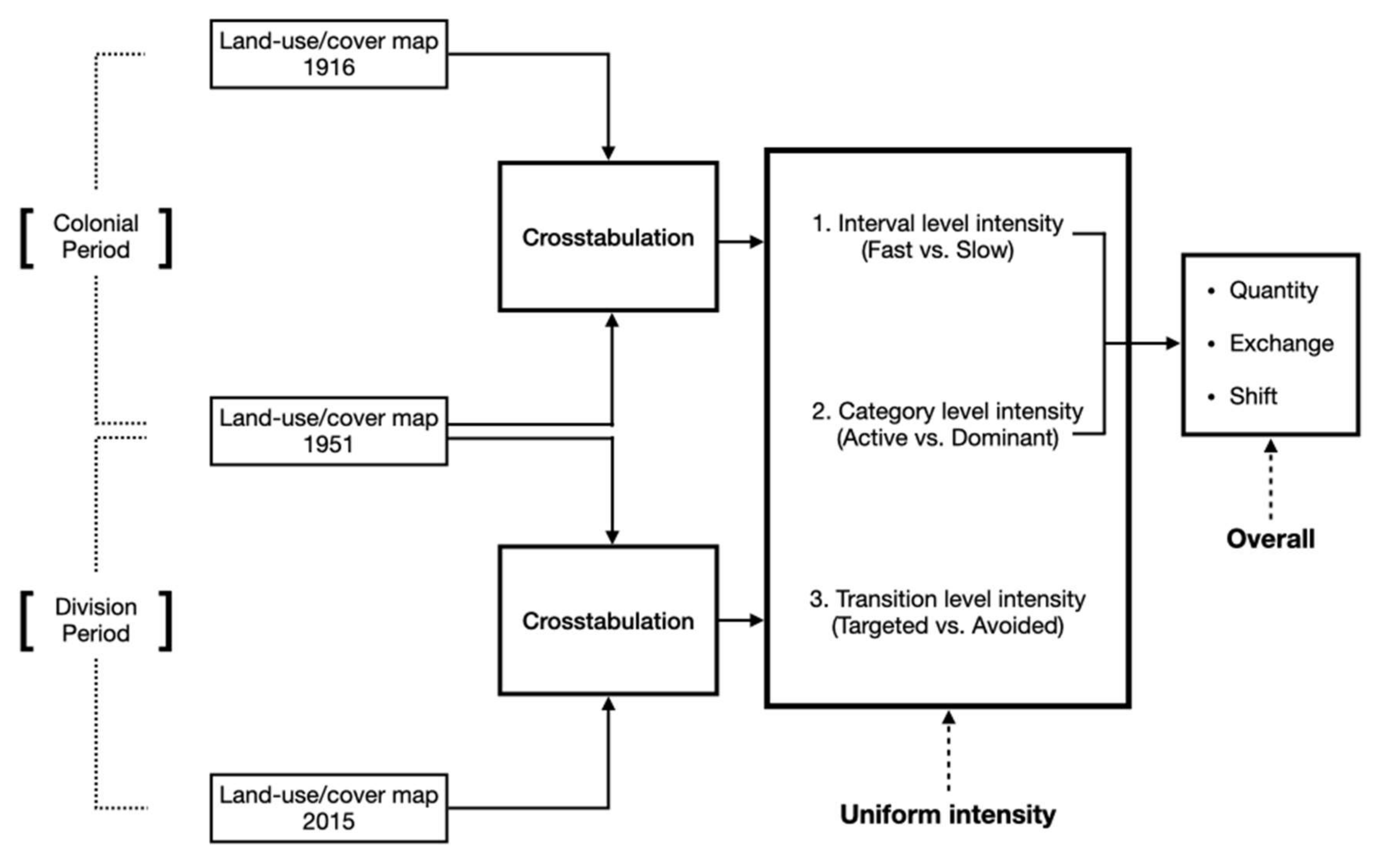
2. Geographical Scope and Land-Use Changes in Kaesong and the DMZ

To acquire insights from the existing literature regarding land cover and land use of Kaesong and the DMZ, it is crucial to understand how their geographical extent have been defined and labeled and whether previous studies examined changes in a spatially explicit manner. We have mapped all of the study areas of the existing literature on Kaesong and the DMZ (Figure 1). Technically distinct areas, Kaesong and the DMZ are adjacent [22]; however, some previous studies have included Kaesong as part of the greater DMZ region [21] (Figure 1). On the other hand, prior research geared towards mapping Kaesong’s land cover and land use based on remotely sensed data has not typically analyzed the entire administrative district of Kaesong in a strict sense but, instead, has focused on the most urbanized area of Kaesong by excluding the surrounding mountains and other non-urban land covers [19,20]. This is typical in the literature, as not all researchers have clearly defined the geographical extent of Kaesong, nor the DMZ, as has been pointed out by our previous research [18,22].
Often in the literature, the Civilian Control Zone (CCZ) is used interchangeably with the DMZ or the Border Region (as specified by South Korean law); however, these terms are not identical. The CCZ is an extra buffer zone of South Korea surrounding the southern boundary of the DMZ to further protect citizens from any potential warfare by restricting the land use, whereas the Border Region is introduced to promote the regional economy of municipalities that have been economically penalized by the CCZ’s restrictions. In terms of jurisdiction, both the CCZ and the Border Region were shaped by South Korea; however, the DMZ is under the command of the United Nations Command Military Armistice Commission [18]. Given these important distinctions, Kim et al. [22] conducted the only study exclusively analyzing the DMZ, although the scope was rather limited in that it only examined the land-cover information of 2013. Seo and Jeon [21] defined the DMZ in two ways: 4 km and 10 km buffer zones from the MDL towards the South and North. By producing the land-cover map for 1996, the authors found that the South Korean side had more built-up areas, whereas the North Korean side had more agricultural lands, revealing distinct land-use and land-cover patterning between the two Koreas.
Limited studies have conducted LUCC analysis along the inner-border region. Park [26] conducted a change detection analysis of the CCZ, generating land-cover maps for 2004, 2010, and 2016 using remote sensing to quantify the LUCCs. The author found that the areas of Built, Agriculture, and Grass had increased, while those of Forest diminished. Subsequently, Park et al. [27] generated and analyzed land-cover maps of 2000, 2009, and 2019, revealing that two wildfires (in 2000 and 2019) substantially contributed to this loss of forest cover. Importantly, none of the previous research relying upon remote sensing data can provide insight on LUCCs prior to the 1970s.

3. Materials and Methods

3.1. Study Area

The economic persistence of Kaesong makes it an ideal site for analyzing LUCCs under the postcolonial and socialist regimes. Kaesong not only is the closest large North Korean city to Seoul and the DMZ but was once the capital of the Goryeo Dynasty (919–1394), where the city functioned as an international and domestic hub for trading goods, particularly Korean ginseng (Panax ginseng). Thus, even during the colonial period, Kaesong was capable of maintaining its leading business and trading position [23,24]. The name “Korea” in fact originated from “Goryeo”, making the city and adjacent areas a World Heritage site certified by the United Nations Educational, Scientific and Cultural Organization (UNESCO) [28].
Following independence from Imperial Japan, Kaesong became part of South Korea, until after the Korean War in 1953 when the city joined North Korea. The South–North Joint Declaration of 15 June 2000 led to the development of the Kaesong Industrial Complex cooperation between the two Koreas; however, its functionality lasted only between 2003 and 2016 when it was abandoned [29].
The study area here includes downtown Kaesong, the first district of the Kaesong Industrial Complex, and the adjacent DMZ area under the North Korean jurisdiction (Figure 1). National security issues notably prevented the inclusion of more areas of the DMZ [18]. The 105.2 km2 study area is split into non-DMZ (96.5 km2) and DMZ (8.6 km2) sections. The study area altitude ranges from 10 to 430 masl, with Kaesong located at 126° 34′ east longitude and 37° 58′ north latitude with an annual mean temperature of 11 °C and precipitation of 1197.1 mm [30].

3.2. Land-Cover Maps

The three years selected for analysis—1916, 1951, and 2015—exemplify critical historical events in Kaesong (Figure 2a–c). The land-cover map of 1916 portrays the undisturbed landscape of Kaesong at the time of colonization by Imperial Japan in 1910, as the detailed land surveys, data processing, compilation, and finally publication (in 1916) all occurred several years before 1916. Similarly, the land-cover map of 1951 describes the region under which the two Koreas became independent, immediately prior to the Korean War-based damage to the landscape. Lastly, the land-cover map of 2015 represents the recent landscape during the South–North division. Accordingly, the study period has been divided into an earlier colonial period (1916–1951) and a latter division period (1951–2015) to be used as input for the intensity analysis. All land-cover maps for each of the three time-steps were previously published by the authors here [18].
As the three land-cover maps are based on separate mapping sources, they specify different land categories. The land-cover maps of 1916 and 1951 are based on old topographic maps (1:50,000) produced by Imperial Japan and the United States Army Map Services, respectively. These old maps were manually digitized using a backward-editing technique [31] based on vector data from 2015 and contain five land categories: Built, Agriculture, Forest, Water, and Others (Figure 2a,b). Built refers to impervious surfaces, namely buildings, transportation infrastructure, and urban settlements; Agriculture refers to primarily rice paddies; Forest is mainly coniferous, with some deciduous stands and orchards; Water includes rivers, lakes, and reservoirs; and Others includes the rest of the land categories such as grasses, barren, and wetlands.
Alternatively, the land-cover map from 2015 is based on remotely sensed data and recent digital topographic maps (1:50,000) provided by South Korean government agencies. The map was similarly manually digitized based on high spatial resolution (2.8 × 2.8 m) satellite imagery acquired from the Korea Multi-Purpose Satellite (KOMPSAT). As reference data, classification outcomes and the digital topographic maps supported the manual digitization to assure maximum accuracy. The land-cover map of 2015 consists of eight land categories: Built, Road, Agriculture, Forest, Grass, Wetland, Barren, and Water (Figure 2c). All three land-cover maps are provided by the Korea Environment Institute [18]. Prior to the intensity analysis, the eight land-cover categories of 2015 were reclassified into the five classes of the 1916 and 1951 maps. Following reclassification, all vector maps were rasterized (30 × 30 m spatial resolution, equivalent to 1:50,000 scale).

3.3. Intensity Analysis

Intensity analyses allow researchers to identify LUCC at three different levels: (1) interval, (2) category, and (3) transition [25]. This assessment improves upon the typical change detection analysis, which identifies areas of change and no-change by comparing at least two land-cover maps from different points in time (i.e., two-way crosstabulation). Intensity analysis methodology does not only consider absolute change (area) but relative change (intensity) as well. Thus, when the three levels are explained in terms of both area and intensity, this framework allows for the acquisition of additional information. Once a measure of intensity is calculated, it is compared to an objective reference (i.e., uniform intensity) to indicate whether the corresponding LUCC is intensive or not [32]. That is, each level has at least one uniform intensity to conclude whether a LUCC is fast or slow (interval level), active or dormant (category level), and targeted or avoided (transition level). Our methodological flow is illustrated in Figure 3.
As for the interval and category levels, areas and intensities are further divided into Quantity, Exchange, and Shift (Figure 3, Appendix A). First, two raster land-cover maps cannot be identical if the number of pixels in an individual land category differ (i.e., unless the quantities of each category are identical, the two maps differ); such a disagreement due to absolute quantity difference is referred to as a difference in “Quantity” [32,33]. Thus, the quantity component measures absolute net change in category area, with all changes pertaining to either gains or losses. Accordingly, the quantity component is less than total gross change when any category experiences simultaneous gain and loss during a time interval.
Second, “Exchange” denotes an allocation disagreement between any two categories [34]. Exchange only considers two categories and does not work for three or more categories. Exchange can be conceptualized as when land category A transitions to land category B in some locations, while B transitions to A in other locations during the same time interval. As the land-cover maps here consist of five classes, ten potential pairwise combinations exist.
Lastly, “Shift” indicates the remaining disagreements, including changes among three or more categories. Accordingly, the overall LUCC is equivalent to the summation of Quantity, Exchange, and Shift [32,33]. In the present research, Quantity, Exchange, and Shift represent “substantial”, “moderate”, and “complex” LUCCs, respectively.
As the transition level of the intensity analysis only considered LUCC gain (not LUCC loss), there were only five transitional outcomes, with each expressed in terms of area and intensity. For each period, the outcomes of change detection analysis are calculated using the Crosstabulation function of TerrSet 2020—a geospatial monitoring and modeling software developed by Clark Labs at Clark University, MA. Changes are computed in terms of area and intensity at the three levels (Figure 3), with further details on all three levels and the associated change components available in Appendix A.

4. Results

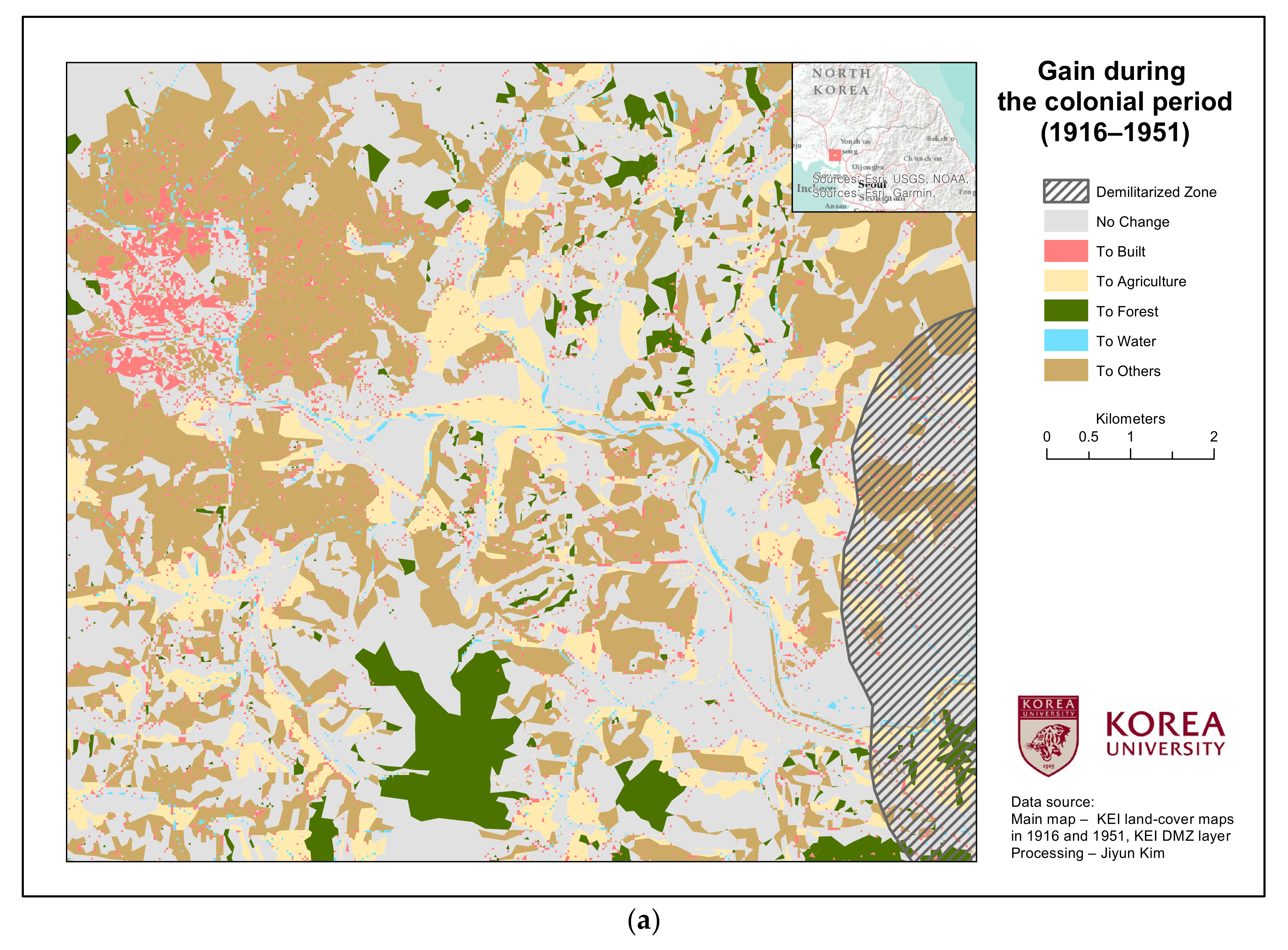
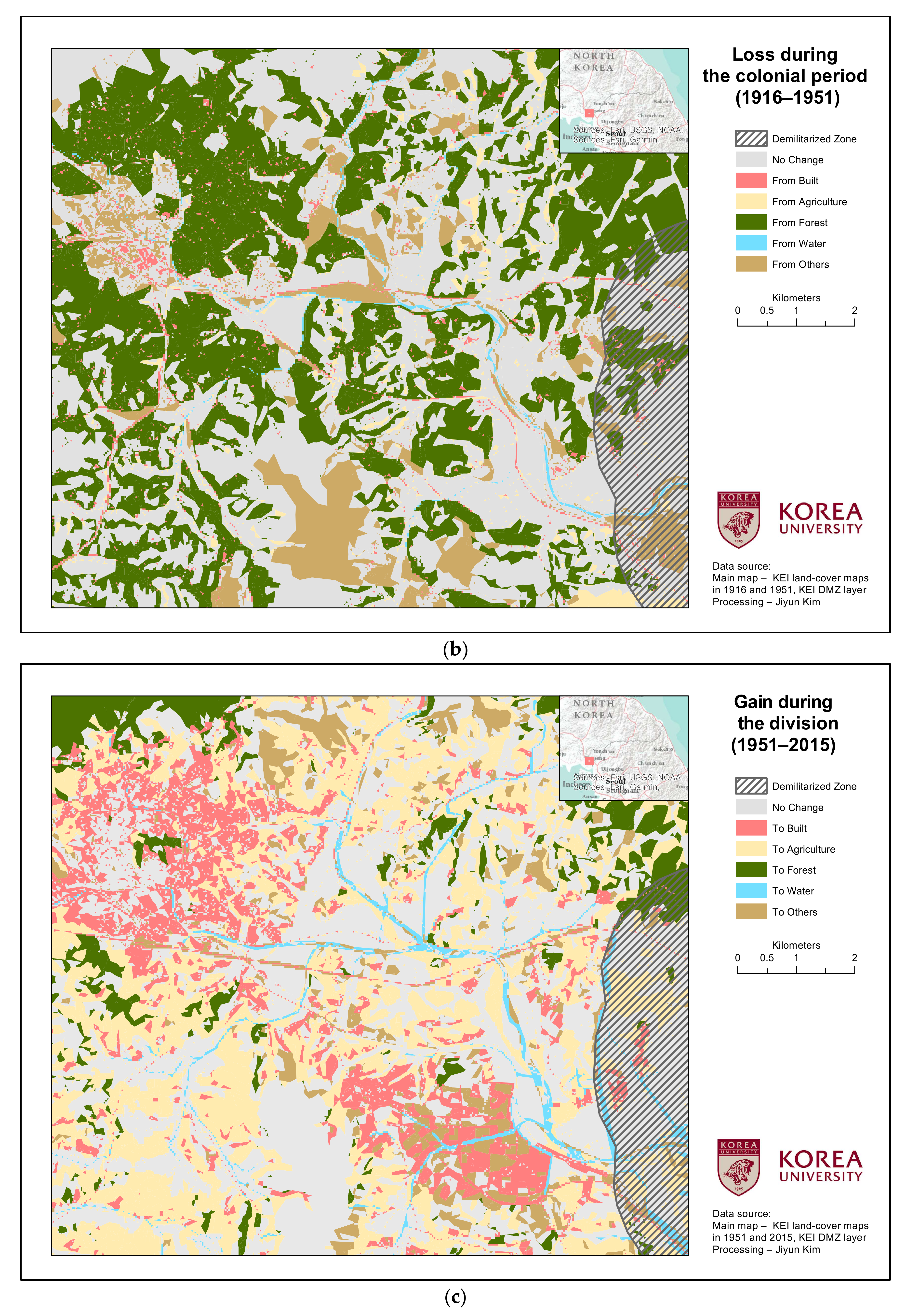
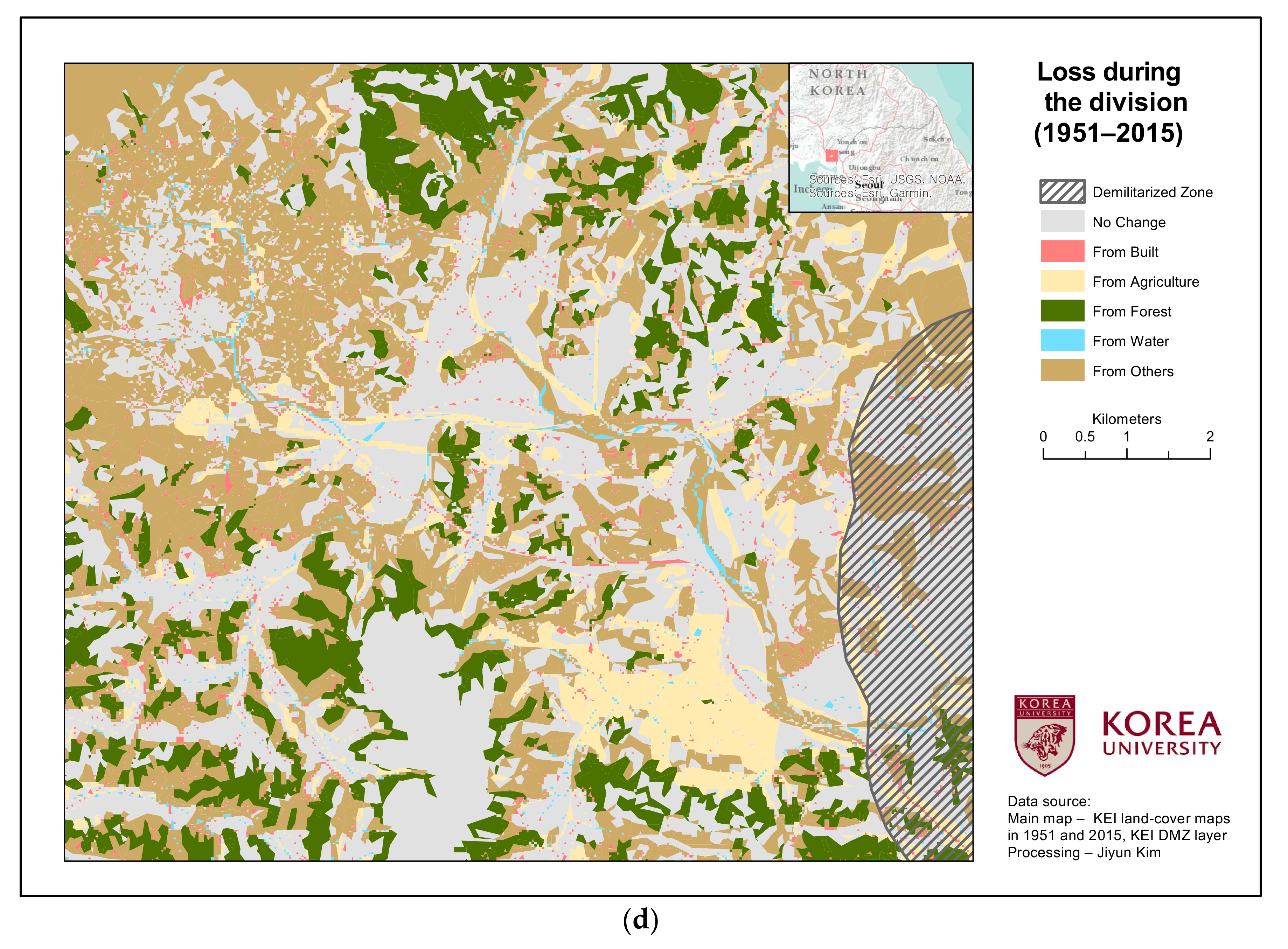
4.1. Change Detection Analysis

First, the areal changes of each category in 1916, 1951, and 2015 are explored. In the study area, Built, Agriculture, and Water continue to increase, whereas Forest continuously decreases from 1916 to 2015. Others shows a mixed pattern (Figure 4).
The transition matrices show LUCCs for each period (Table 1) and are used as inputs for the intensity analysis (spatial representations are shown in Figure 5a–d). Figure 5a,b demonstrate gain and loss, respectively, during the colonial period, (Table 1), thereby showing how the original landscape of Kaesong was altered under colonization. The most significant LUCC in terms of area was deforestation (gross Forest loss = 41.51 km2); however, minor afforestation activities were also observed across the same period (gross Forest gain = 5.60 km2; Table 1). The primary contribution to Others gain was deforestation (Figure 5a,b; Table 1). While the deforestation took place around flat and low urban areas, afforestation was observed in the hilly regions. As a result, the urbanized downtown of Kaesong became larger, with the study area also becoming more cultivated during this colonial period (Figure 5a).
Figure 5c,d similarly display gain and loss, respectively, during the division, with their accompanying LUCCs summarized in Table 1. Agriculture had the biggest LUCC gain (31.38 km2), followed by Built gain (13.42 km2; Table 1). Areas that had been deforested during the colonial period were mostly used for cultivation (rice paddies) during the division period (Figure 5a–d). Downtown Kaesong also grew larger, suggesting consistent urbanization. Further, hosting the Kaesong Industrial Complex in the region contributed to the addition of Built gain (Figure 5c). The other LUCCs also showed substantial gains; for example, Water increased by 2.60 km2, as the major river stream straightened and widened, highlighting the major construction and civil engineering activities in the area. Gains in Forest (9.08 km2) were observed in the hilly areas, with a small patch of Forest gain identified in the middle of downtown Kaesong (i.e., urban forest; Figure 5c). However, Forest loss in the flat areas was observed as well primarily due to agricultural cultivation (Figure 5d).
Within the DMZ, categories of Built, Agriculture, Forest, and Water increased in area (Figure 5c) by mostly converting from Forest and Others categories (Figure 5d). The LUCCs within the DMZ patch were relatively substantial, considering that human activities in the area are highly limited due to military tensions between South and North Korea (Figure 5c,d).

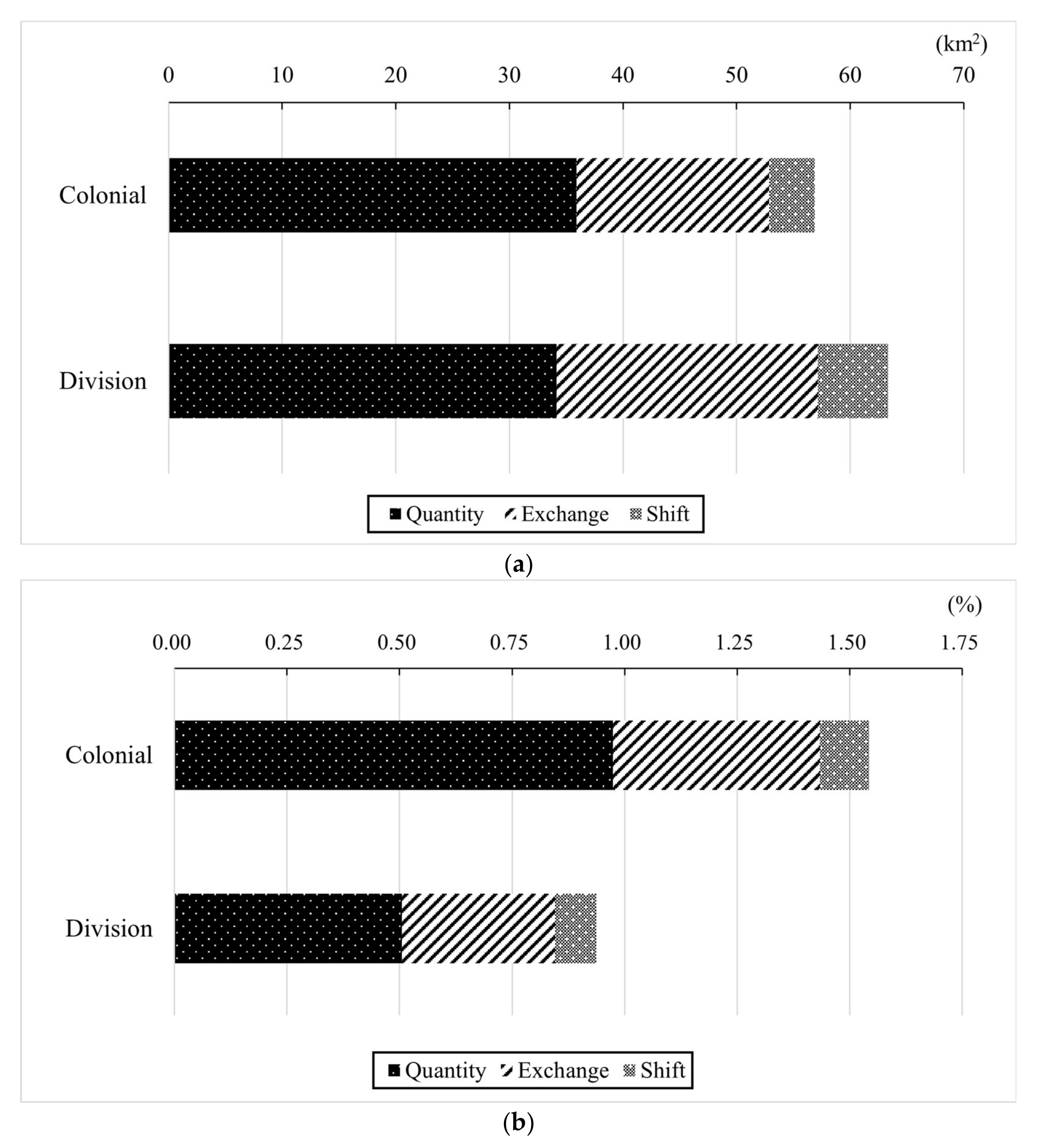
4.2. Interval Level Intensity

The outcome of the interval level is twofold: (1) the first measure quantifies the rate of LUCC over a given period, as determined by the two land-cover maps (where the length of the time window can be arbitrary); and (2) the second measure normalizes the former to yield an annual rate of LUCC (i.e., intensity), as the two time windows have different lengths (namely, 35 and 64 y). Both measures employ different time windows as the denominator for an individual LUCC (the numerator). Notably, the division period showed greater LUCCs than the colonial period; however, when normalized, the colonial period underwent more intense changes than the division period. In total, >50% of the study area experienced changes across the entire study period (Figure 6).
LUCCs in terms of area and intensity (Figure 6) are further decomposed into Quantity, Exchange, and Shift (Figure 7a–c). Quantity drives the majority of the LUCCs, followed by Exchange and Shift, regardless of the historical period being examined, thus indicating substantial LUCCs across both periods. As stated, the colonial period showed greater Quantity than the division period by total area (Figure 7a); however, when normalized to intensity, Quantity of the colonial period is two times larger (Figure 7b). Quantity Overall shows an identical pattern, where the landscape underwent more substantial changes during the colonial period (Figure 7c).

4.3. Category Level Intensity

Among all land categories, Forest was the only net loss during colonization (Figure 8a). Consequently, the other land categories revealed net gain (Figure 8b; Table 2). Forest showed the largest loss (41.51 km2), whereas Others maintained the largest gain (33.29 km2; Figure 8a). Comparatively, the LUCCs of other categories were relatively minor, although Built and Agriculture indicated some gains. During the division period, Agriculture showed the most substantial gain (31.38 km2), followed by Built (13.42 km2), representing increased gains of 20.17 km2 and 7.94 km2 over the previous period, respectively. The Others class lost considerable area and gained little. Further, Forest loss during the division was less than that in the colonial period (Figure 8a).
Forest loss during the colonial period was substantial and active in terms of intensity (Figure 8b); however, the loss of Forest (2.06%) was not more active than that of Water (2.29%). Further, Forest loss was no more intense than Built loss (2.05%) in terms of intensity. By linking such intensity outcomes to the data presented in Figure 8a, it is reasonable to conclude that Forest change was relatively less severe than other classes (i.e., its quantity loss was large due to its greater initial area). If the size of a land category is large, it is expected to show extensive changes even with moderate intensity. Thus, deforestation in the study area during the colonial period was less extreme compared to Water and Built (Figure 8b); when considering gains as well, the LUCCs of these two classes were more active than that of Forest (Figure 8b).
As mentioned, Forest loss during the division was smaller than that during the colonial period by area (Figure 8a). In terms of intensity, however, Forest loss during the division was not minor (i.e., the loss was active; Figure 8b). Agriculture gain shows the opposite pattern, where in terms of size, its gain was substantial (Figure 8a), but these changes were barely active in terms of intensity (Figure 8b). Water gain (1.41%) was still most active during the division, followed by Others loss (1.32%) and Built gain (1.28%). Water was the only category in which both gains and losses were active (Figure 8b).
Forest during the colonial period (Figure 9a) shows the largest LUCC by area (47.10 km2), largely a result of its Quantity (35.90 km2). This is followed by Others (42.65 km2), where Quantity (23.94 km2) is also the largest change component. Agriculture similarly shows more Quantity than the other two components, whereas Built and Water demonstrate more Exchange than Quantity (Figure 9a). During the division (Figure 10b), Others shows the largest LUCC (42.68 km2), followed by Agriculture (40.03 km2), for which Quantities contributed to the majority of both changes (28.98 km2 and 22.72 km2, respectively). In this latter period, Built also shows greater Quantity than the other two components, indicating more substantial one-way changes compared to the colonial period (Figure 9a,b). As for Forest and Water, Exchange is the major contributor to their LUCCs (Figure 9b). Further, while no Shift was observed for Forest during the colonial period (Figure 9a), more Shift than Quantity was seen during the division (Figure 9b).
In the colonial period, Quantities of Forest, Agriculture and Others were larger than Quantity Overall, implying that one-way change was substantial for these three land categories in terms of intensity. Exchanges of Built and Water were larger than Exchange Overall, suggesting more moderate LUCCs. Shifts of Others and Agriculture were found to be greater than Shift Overall, implying more complex LUCCs (Figure 10a; Table 3). During the division, Others, Built, and Agriculture showed larger Quantities than Quantity Overall (Figure 10b; Table 3), whereas Exchange of Water was larger than Exchange Overall, and Only Forest’s Shift was larger than Shift Overall.
In summary, Agriculture and Others showed substantial one-way LUCC across both periods. Notably, the direction of Others during the colonial (gain) and the division (loss) periods is reversed.

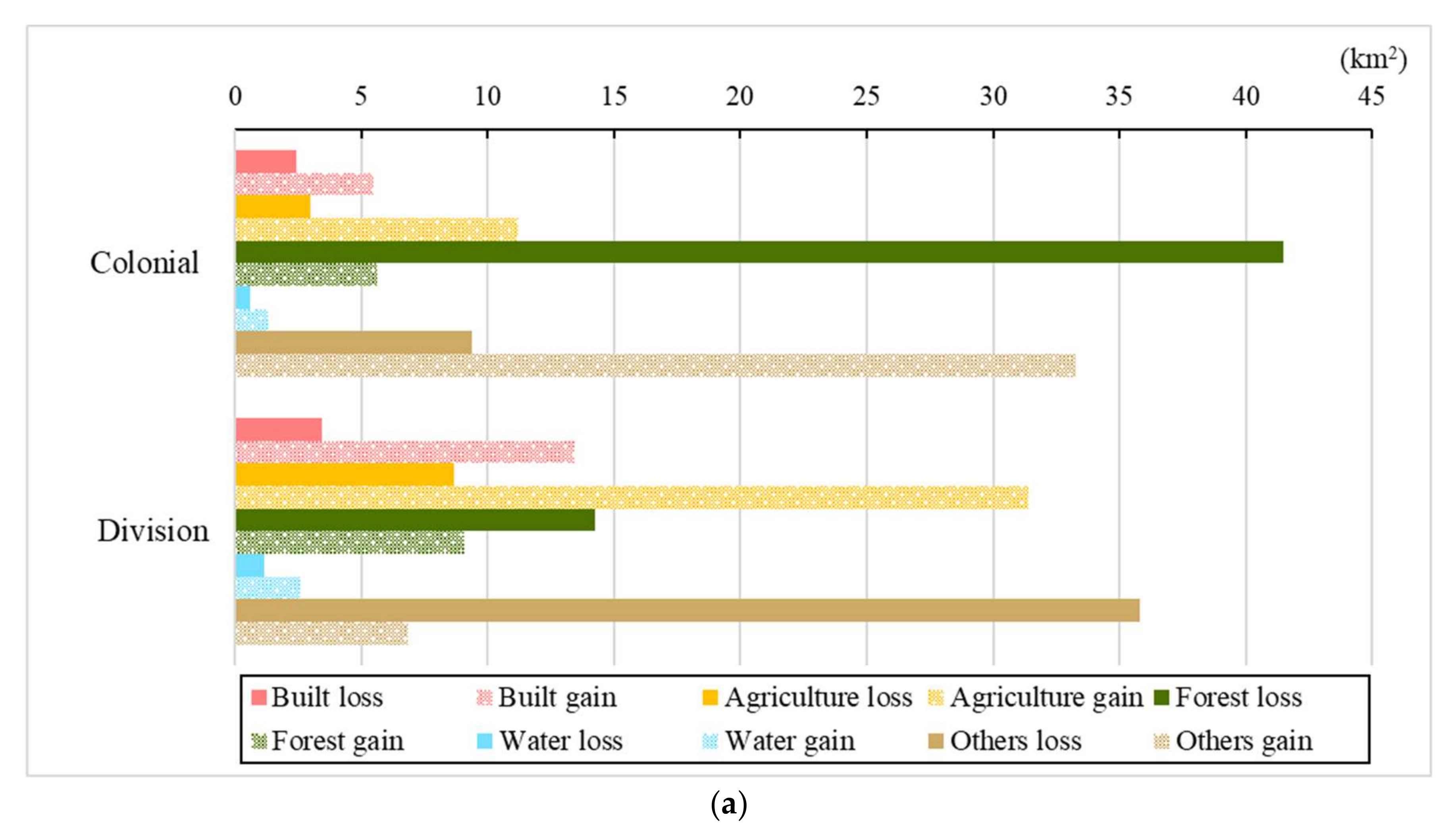
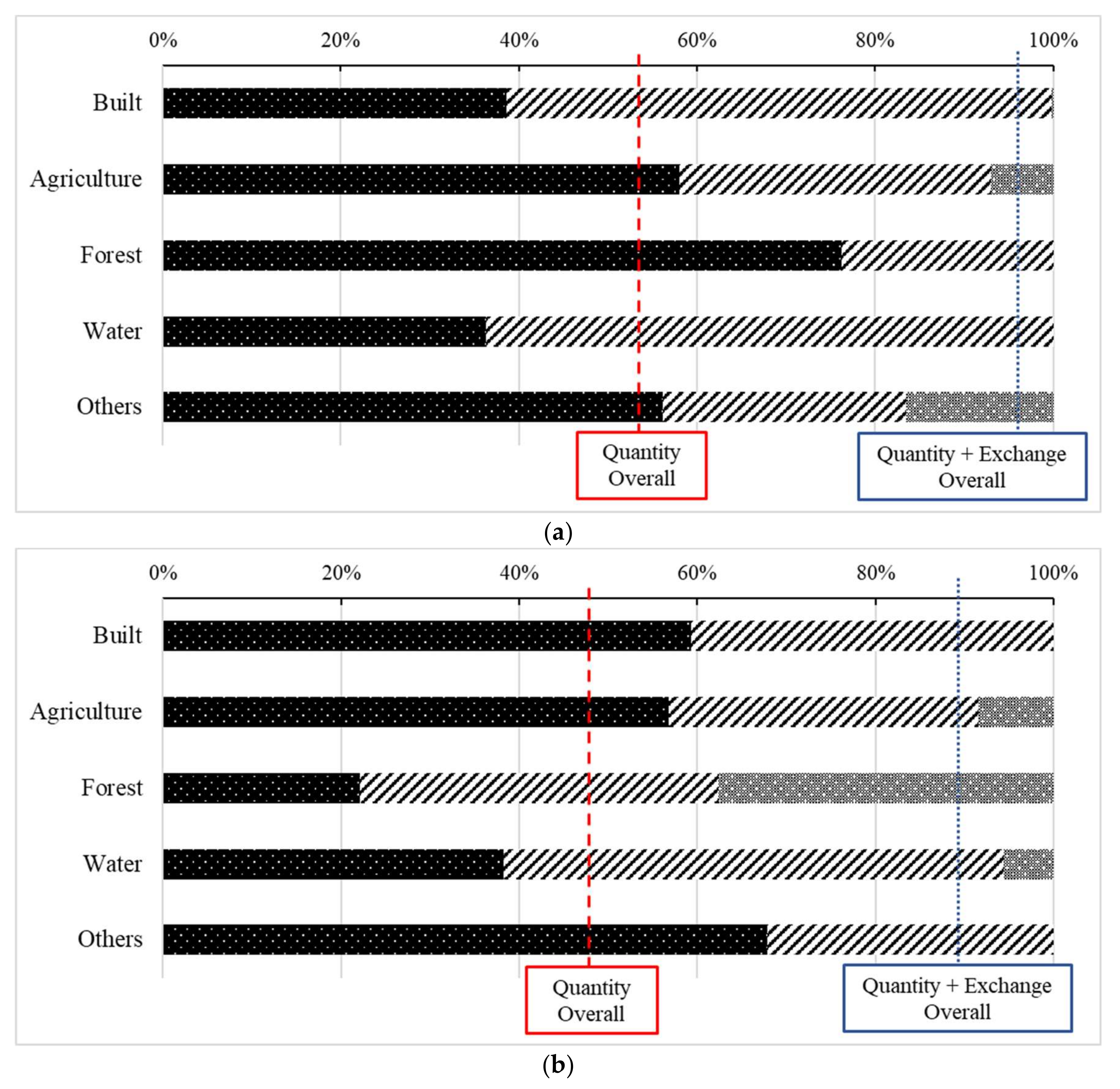
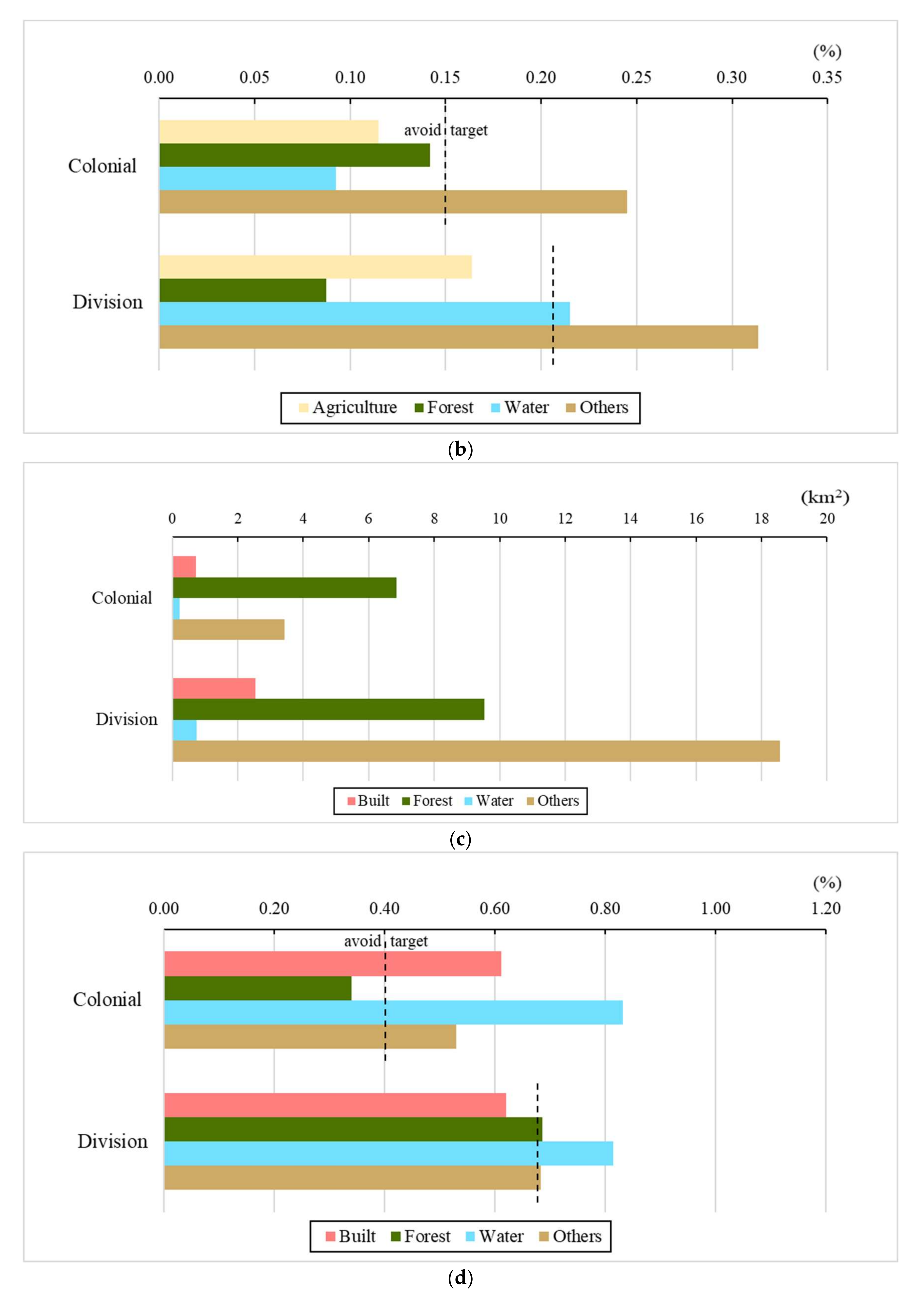
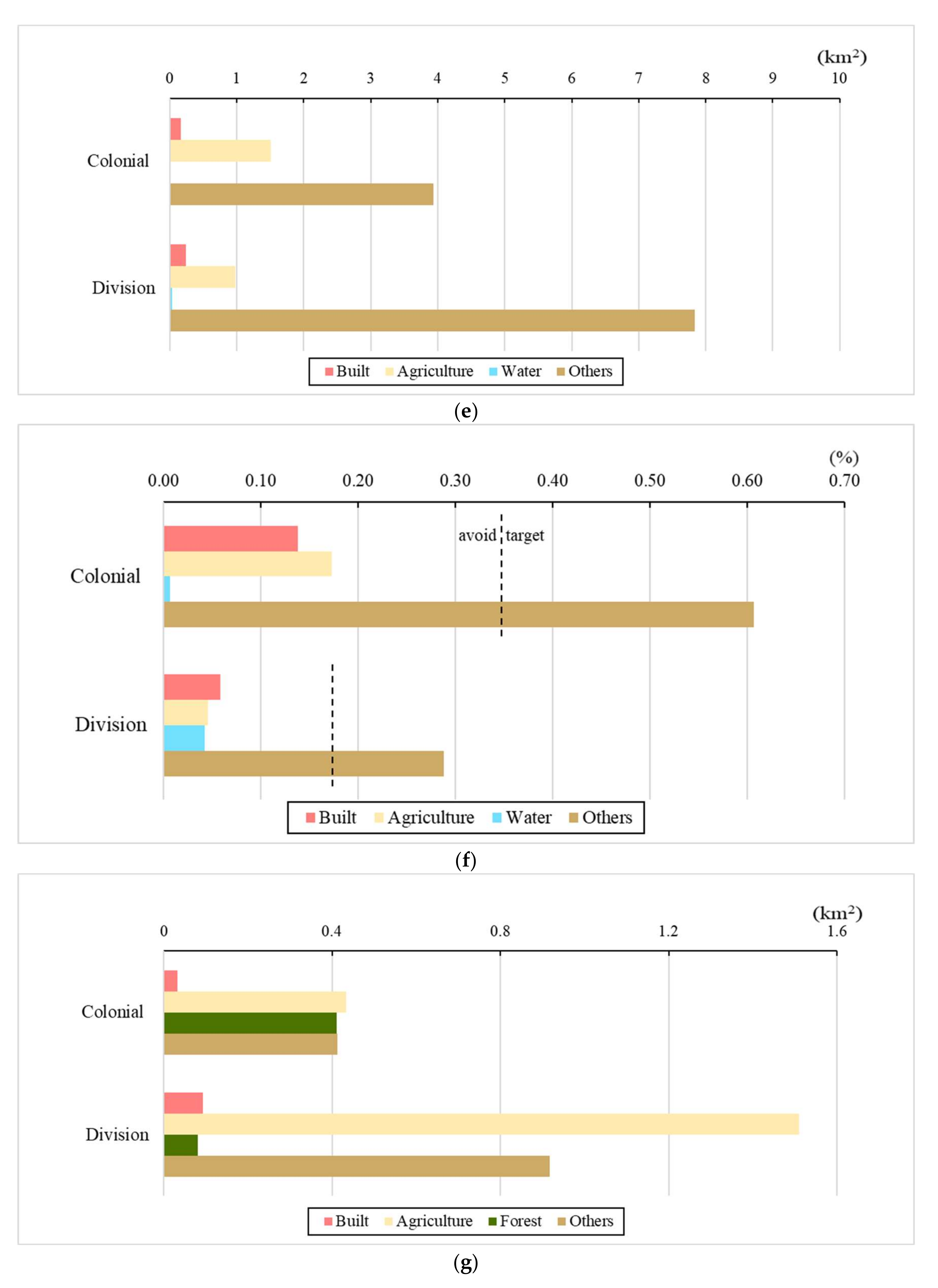
4.4. Transition Level Intensity

In the colonial period, Forest had the largest area converted to Built. However, in terms of intensity, only the Others category was targeted in the colonial period (Figure 11b), with Forest avoided. During the division, Others contributed the most to Built (Figure 11a), with a similar trend observed for intensity. Further, Water was also targeted by Built in terms of intensity (Figure 11b).
Agriculture targeted mostly Forest during the colonial period (Figure 11c), whereas, for intensity, Agriculture targeted all of the other land categories, except Forest (Figure 11d). During the division period, Agriculture targeted all but Built (Figure 11d), whereas the LUCC from the other categories to Agriculture is more notable among the transitions, being largely a result of greater area and intensity (Figure 11a–j).
The transition to Forest was the only case in which the outcomes in terms of area and intensity were aligned. Only Others was targeted for both periods (Figure 11e,f). In terms of the transition to Water, Agriculture was consistently targeted in both periods, while the outcomes in terms of area and intensity were aligned. Water consistently targeted Agriculture (Figure 11g,h), while Others was targeted more than Agriculture only during the colonial period (Figure 11h).
In the transition to Others, Forest and Water were consistently targeted across both periods, with comparable outcomes in terms of area and intensity. Conversely, Agriculture was always avoided (Figure 11i,j), while Built was only targeted during the colonial period (Figure 11j).

5. Discussion

A series of intensity analyses was conducted to understand how land uses and land covers were changed in Kaesong, North Korea, with respect to two important historical periods. It is evident that Kaesong’s LUCC was relatively faster and substantially more intensive during the colonization period by Imperial Japan compared to that when it fell under the jurisdiction of North Korea; however, the division period still showed a marked LUCC in an absolute sense. More than half of the study area experienced changes, regardless of the land regimes. Although deforestation may be responsible for the majority of LUCC in Kaesong, Water showed the most intensive changes of all categories. This outcome indicates that the river channel was consistently modified underneath Imperial Japan and North Korea. In terms of transition, there was always at least one land category that contributed the most to another. Such targeted patterns were observed regardless of the land regimes across the different periods, implying that there may be underlying forces driving LUCCs in Kaesong outside the influence of the land regime.
Kaesong is one of the wealthiest and most populated North Korean cities. This is in part because the city hosts the large-scale factory co-operated by the South and the North (i.e., Kaesong Industrial Complex, although the factory ceased operations in 2016), and partly because traditionally Kaesong has been an active business and trading center [23]. Given the context, the outcome of more active development of Kaesong during colonialism than under North Korean jurisdiction is unexpected. This result may also imply that the majority of North Korean cities, except the capital, Pyongyang, may be still largely underdeveloped as their urban growth since the Korean War has been more controlled and less intensive than during the colonial period. Although it is rather uncertain, Kaesong’s less active development during the division period may be in part due to decreasing urban population. According to Statistics Korea [35], the population of Kaesong decreased from 334,433 inhabitants in 1993 to 308,440 in 2008. However, large uncertainties are embedded in the census data, as military personnel are not accounted for in population statistics [36], and it is likely that a substantial number of North Korean soldiers live in Kaesong.
Both Imperial Japan and North Korea had/have centralized land-use policies, and the patterns of LUCC having much Quantity across both land regimes empirically showed LUCC in Kaesong occurred in line with national policies and strategies. In October 1976, the North Korean government officially announced a fundamental nature-reorganization policy for renewing and strengthening North Korea as a socialist country [37] (p111). The policy includes terraced upland cultivation, as well as land rearrangement and improvement for increasing agricultural production. The terraced upland cultivation policy had a target transition of 200,000 ha with >16° slope to upland fields on a national scale [20] (p57). Specifically, it was the Land Law of 1977 that encouraged the cultivation of terraced uplands [38] (p5170). Thus, the terraced upland cultivation policy supported the conversion of Forest to Agriculture in Kaesong, whereas the nature-reorganization policy similarly included land rearrangement projects containing intensive land transformation around the river for expanding agricultural lands [20] (p57). River projects were also conducted for straightening and widening river channels in North Korea, driven by river management policies that have controlled the transition of Water to Agriculture and Agriculture to Water in Kaesong.
North Korea is one of the most deforested nations [39]. Accordingly, it was found here that forest loss in Kaesong was active in both periods. Surprisingly, however, the findings showed that the river channel experienced more intensive change than deforestation. Furthermore, the analysis revealed that in terms of intensity, Kaesong and DMZ experienced considerable Water gain and loss, a finding typically omitted from previous studies. Some of Water’s gain during the colonial period can be explained by civil engineering projects in Kaesong. According to the Chosen Government General of Imperial Japan [40], major civil engineering constructions were conducted on two river streams (Yangseong-cheon and Jipari-cheon) to prevent damage to residential and agricultural areas, as well as transportation infrastructure due to frequent flooding during monsoon seasons. As a result, the LUCCs due to such major undertakings appear as gains in the Water category (Figure 6a). During the division period, the construction of Kaesong Industrial Complex resulted in modifying the river channel yet again to supply water to the city and factories (Jeong, S.K. Personal communication, 2019).
The consistent LUCC transitions trends of intensity, regardless of land regimes, are as follows: Others to Built, Water and Others to Agriculture, Others to Forest, Agriculture to Water, and Forest and Water to Others (Figure 11a–j). It is logical to infer that these transitions are driven by more fundamental underlying forces of LUCC than the land regimes (imperialism and socialism). Thus, we argue that such forces are economic and geographic factors. For example, the transition from Others to Built is likely driven by economic factors. Given that the Others category includes grass, barren, and wetlands, the category is prone to be used for building residential areas and installing transportation infrastructure. The transition from Forest to Others are likely driven by economic factors, with respect to energy and food. Deforestation and forest degradation typically occur when people collect biomass to use as fuel for cooking and heating, or when deforested lands are converted to agriculture [39,41]. Alternatively, the transitions of Water and Others to Agriculture, Agriculture to Water, and Water to Others are likely shaped by geography (Figure 6a–d). As the Others category includes wetlands along the river, the exchange between these categories is likely driven by civil engineering projects in both periods. Such exchanges occur primarily because Water, Others (wetlands), and Agriculture are adjacent to each other. Agriculture lands are typically located along rivers, as the geographical proximity allows for more efficient channeling of water to rice paddy fields.
The transition from Others to Forest in Kaesong indicates planned reforestation activities rather than land abandonment, which were commonly observed in Europe after the collapse of the Eastern Bloc [42,43,44,45,46,47,48]. In Kaesong, reforestation activities for both periods are often identified in the hilly regions of the study area (Figure 5a–d). Thus, it is unlikely that this transition would be driven by land abandonment, as one of the general LUCC trends in Kaesong was that much of the hilly land, even on less productive soils, was converted to agriculture (Figure 8a). Similar trends of increasing farmland extent have been observed in the Czech Republic [46], Slovakia [44], and Ukraine [45] while they were under a socialist political system. However, following the introduction of modern democratic and capitalist systems to Eastern Europe, land abandonment became more common as agricultural practices on less productive lands were no longer economically viable, in addition to substantial emigration from rural areas [43,44,45]. The sociopolitical transformation and new socioeconomic conditions in Hungary and Poland after 1989 have contributed significantly to the decrease of agricultural land and the increase of forest and uncultivated land coverage [48]. Given the findings here, and the persistent system of centralized planning, it is inferred that land abandonment in Kaesong has been rather limited. After the Korean war, Kaesong was intensively developed by the governmental design and control in restoring historical and cultural places and arranging public facilities [24].
Several researchers have studied Kaesong’s land cover, but no research presented findings similar to our present work. The first case study on Kaesong’s land cover mapped numerous types of land covers in 2000 based on an IKONOS image [20]. The research was considered relatively novel then, at least from a non-military perspective. Similar research was conducted more than a decade later [19]. It spatially visualized multiple types of land covers of Kaesong based on the Korean Multi-Purpose Satellite but with a broader geographical scope, compared to Kim et al. [20]. While these two studies demonstrated only the land categories of Kaesong for each year, Kang et al. [16] analyzed the change of Built areas in Kaesong, along with the other nine large cities in North Korea. According to the authors, Kaesong’s urbanization was more intensive in the 1980s–1990s than the 1990s–2000s, only analyzing LUCCs during the South–North division. Our previous work also studied LUCCs in Kaesong using identical data to our present work, but the quantification of LUCC was limited, so it was difficult to argue which historical period impacted the landscape more intensively than the other [18].

6. Conclusions

In this study, we found that multiple aspects of Kaesong’s LUCCs during the colonial period were more intensive than those during the South–North division period, implying that LUCC under the socialist regime has been less dynamic than under Japanese colonization in this region of the Korean Peninsula. However, >50% of the study area underwent changes in both periods, with the river channel modification and deforestation being the most substantial. Our results also indicate that Kaesong has been developed and urbanized under controlled land-use planning which recognized the historical values of the city. In addition, the applied intensity analysis allowed us to examine specific LUCC patterns in Kaesong and interpret them in the context of national policies focusing on underlying drivers of land use. It was thus concluded that LUCC was more intensive under colonialism than socialism; however, the examined land regimes did not substantially affect the underlying economic and geographic driving forces of change.
The present research contributes to extending our collective understanding of LUCCs in the context of different conditions and political regimes in North Korea through time. To better enhance this knowledge, more case studies are required, combining land change intensity with detailed policy analyses. Ideally, future research should target multiple case studies that would provide a more representative sample of LUCC at the national level. Simultaneously, future studies should use data of a temporal scale closely reflecting the implementation of the various influential national policies controlling land-use dynamics in North Korea, such as the Sloping Land Management Program or the National Agroforestry Policy and Strategy.

Author Contributions

Conceptualization, O.S.K. and M.N.; methodology, O.S.K., T.V. and M.N.; formal analysis, O.S.K.; data curation, O.S.K. and M.N.; writing—original draft preparation, O.S.K., T.V. and M.S.P.; writing—review and editing, O.S.K., T.V., M.S.P. and M.N.; visualization, O.S.K.; supervision, O.S.K., T.V., M.S.P. and M.N.; funding acquisition, O.S.K. All authors have read and agreed to the published version of the manuscript.

Funding

O.S.K. was supported by the Korea University Grant (College of Education 2022). T.V. was supported by grant IGA_PrF_2021_014 (Palacký University Olomouc). The APC was funded by T.V.

Acknowledgments

We are very grateful to Safaa Aldwaik and Gil Pontius, Jr. for sharing their code via http://www.clarku.edu/~rpontius/ (accessed on 8 February 2021). Clark Labs supported our work by developing TerrSet 2020. We also thank Keumsoo Hong at Korea University for his generous support in searching historical documents. We acknowledge J Kim’s assistance with producing figures and tables.

Conflicts of Interest

The authors declare no conflict of interest.

Appendix A

Appendix A.1. Interval Level Intensity

Intensity at the interval level and its uniform intensity are defined according to the following:
I f , l = s i z e   o f   C h a n g e   d u r i n g   y e a r f , y e a r l × 100 s i z e   o f   s t u d y   a r e a   d u r a t i o n   o f   y e a r f , y e a r l
U I = s i z e   o f   C h a n g e   d u r i n g   a l l   i n t e r v a l s × 100 s i z e   o f   s t u d y   a r e a   d u r a t i o n   o f   a l l   i n t e r v a l s
where I f , l denotes the intensity between the former year ( y e a r f ) and the latter year ( y e a r l ), and U I refers to the interval level uniform intensity (a notably hypothetical change, and not necessarily observed). If I f , l < U I , it means that LUCC at the given time interval (between the former year and the latter year) is “slow” compared to the average annual LUCC in the study area when all changes across the entire time period are distributed equally annually. Conversely, if I f , l > U I , this means that LUCC at the given time interval is “fast”. LUCCs at the interval level are further specified into Quantity, Exchange, and Shift in terms of area and intensity.

Appendix A.2. Category Level Intensity

At the category level, the number of gains and losses are quantified for each land category and for each time interval as follows:
L f , l , i = s i z e   o f   l o s s   o f   i   d u r i n g   y e a r f , y e a r l × 100   s i z e   o f   i   i n   y e a r f   d u r a t i o n   o f   y e a r f , y e a r l
G f , l , j = s i z e   o f   g a i n   o f   j   d u r i n g   y e a r f , y e a r l × 100 s i z e   o f   j   i n   y e a r l   d u r a t i o n   o f   y e a r f , y e a r l
where L f , l , i indicates the intensity of category i’s loss between the former year and the latter year, and G f , l , j refers to the intensity of category j’s gain for the same period. Specifically, category i points to the category in the former year that experienced loss in the latter year. That is, over time, category i is converted into another category. Similarly, category j indicates the category in the latter year that experienced gain from non-j categories in the former year.
Here, it is important to note that I f , l functions as the uniform intensity for each time interval at the category level. Therefore, L f , l , i and G f , l , j are compared with the uniform intensity, I f , l . If L f , l , i < I f , l , LUCC is considered “dormant”, meaning that category i changed less intensively than the uniform intensity for the given time period. Alternatively, if L f , l , i > I f , l , LUCC is “active”, meaning that category j changed more intensively than the uniform intensity for the same period. Similarly, if G f , l , j < I f , l or G f , l , j > I f , l , this means LUCC gain has been dormant and active, respectively.
LUCCs at the category level are further divided into Quantity, Exchange, and Shift in terms of area and intensity. These change components do not distinguish between gains and losses; therefore, this approach is geared towards dictating how intensive each LUCC had been in either direction. At the category level, Quantity dictates the relatively substantial one-way LUCCs, because if the magnitude of LUCC does not exceed any two categories’ trade, there cannot be any substantial Quantity. Exchange, by definition, occurs when two land categories swapped the exact number of pixels (equal areas); thus, it depicts a moderate LUCC dynamic. Such dynamics are relatively simple compared to Shift, which illustrates a complex LUCC, including but not limited to changes between more than two land categories.
As LUCC in terms of area is further specified into Quantity, Exchange, and Shift, LUCC in terms of intensity can be further divided into the three change components as well. Accordingly, a type of uniform intensity for each component is required and is represented here by Quantity Overall, Exchange Overall, and Shift Overall, which collectively sum up to 100%. Quantity Overall denotes the ratio of overall Quantity across all LUCCs, with Exchange Overall and Shift Overall defined similarly. In brief, if Quantity of Built is more than Quantity Overall, it means that Built’s LUCC is “substantially one-way”. If not, the change is viewed as insubstantial. Similarly, if Exchange of Built is more than Exchange Overall, it means that Built’s LUCC is “moderate”. Lastly, if Shift of Built is larger than Shift Overall, it means that Built’s LUCC is “complex”. Because the order of proportion of Quantity, Exchange, and Shift in terms of intensity is identical to the order in terms of area, it is not necessary to compare the change components’ area to intensity but rather to compare the intensities of the three change components to their Overall values.

Appendix A.3. Transition Level Intensity

While a category level intensity does not provide information regarding which category has changed into another, a transition level intensity demonstrates this additional information regarding the direction of LUCC. At the transition level, it only considers the gain in the latter year because all possible transitions inherently take into account the former year’s losses. Both the transition level intensity and its uniform intensity are derived according to the following:
T f , l , i , n = s i z e   o f   t r a n s i t i o n   f r o m   i   t o   n   d u r i n g   y e a r f , y e a r l × 100 s i z e   o f   i   i n   y e a r f   d u r a t i o n   o f   y e a r f , y e a r l  
U T f , l , n = s i z e   o f   g a i n   o f   n   d u r i n g   y e a r f , y e a r l × 100 s i z e   o f   n o t   n   i n   y e a r f   d u r a t i o n   o f   y e a r f , y e a r l  
where T f , l , i , n is the intensity of transition from categories i to n and, compared to U T f , l , n , the uniform intensity at the transition level given the gain of category n. This comparison makes it possible to evaluate whether or not a conversion from one category into another is intensive (i.e., if the observed intensity of each transition is targeted or avoided).
If T f , l , i , n < U T f , l , n , the transition is “avoided”, meaning that category i targets category n less intensively, when compared to the area that category n gained uniformly from the area of non-n category throughout the former year (i.e., the uniform intensity). Thus, category i in the former year does not contribute disproportionately to the gain of category n in the latter year when compared to the other non-n categories. If T f , l , i , n > U T f , l , n , the transition is “targeted”, meaning that the change from categories i to n is more intensive than the uniform intensity. For example, the uniform intensity of “To Built” between 1916 and 1951 is identical to the ratio of “non-Built” in 1916.

References

  1. Meyfroidt, P.; Chowdhury, R.R.; de Bremond, A.; Ellis, E.; Erb, K.-H.; Filatova, T.; Garrett, R.; Grove, J.; Heinimann, A.; Kuemmerle, T.; et al. Middle-range theories of land system change. Glob. Environ. Chang. 2018, 53, 52–67. [Google Scholar] [CrossRef]
  2. Veldkamp, A.; Verburg, P. Modelling land use change and environmental impact. J. Environ. Manag. 2004, 72, 1–3. [Google Scholar] [CrossRef]
  3. Lambin, E.F.; Turner, B.L.; Geist, H.J.; Agbola, S.B.; Angelsen, A.; Bruce, J.W.; Coomes, O.T.; Dirzo, R.; Fischer, G.; Folke, C.; et al. The causes of land-use and land-cover change: Moving beyond the myths. Glob. Environ. Chang. 2001, 11, 261–269. [Google Scholar] [CrossRef]
  4. Meerow, S.; Newell, J.P.; Stults, M. Defining urban resilience: A review. Landsc. Urban Plan. 2016, 147, 38–49. [Google Scholar] [CrossRef]
  5. Seto, K.C.; Güneralp, B.; Hutyra, L.R. Global forecasts of urban expansion to 2030 and direct impacts on biodiversity and carbon pools. Proc. Natl. Acad. Sci. USA 2012, 109, 16083–16088. [Google Scholar] [CrossRef] [Green Version]
  6. Montgomery, M.R. The urban transformation of the developing world. Science 2008, 319, 761–764. [Google Scholar] [CrossRef] [Green Version]
  7. Quan, B.; Pontius, R.G., Jr.; Song, H. Intensity Analysis to communicate land change during three time intervals in two regions of Quanzhou city, China. GIScience Remote Sens. 2020, 57, 21–36. [Google Scholar] [CrossRef]
  8. He, J.; Xu, J. Is there decentralization in North Korea? Evidence and lessons from the sloping land management program 2004–2014. Land Use Policy 2017, 61, 113–125. [Google Scholar] [CrossRef]
  9. Huang, X.; Schneider, A.; Friedl, M.A. Mapping sub-pixel urban expansion in China using MODIS and DMSP/OLS nighttime lights. Remote Sens. Environ. 2016, 175, 92–108. [Google Scholar] [CrossRef]
  10. Schneider, A.; Mertes, C.M.; Tatem, A.J.; Tan, B.; Sullamenashe, D.; Graves, S.J.; Patel, N.N.; Horton, J.A.; Gaughan, A.E.; Rollo, J.T.; et al. A new urban landscape in East–Southeast Asia, 2000–2010. Environ. Res. Lett. 2015, 10, 034002. [Google Scholar] [CrossRef]
  11. Schneider, A.; Mertes, C.M. Expansion and growth in Chinese cities, 1978–2010. Environ. Res. Lett. 2014, 9, 024008. [Google Scholar] [CrossRef]
  12. Kontgis, C.; Schneider, A.; Fox, J.; Saksena, S.; Spencer, J.H.; Castrence, M. Monitoring peri-urbanization in the greater Ho Chi Minh city metropolitan area. Appl. Geogr. 2015, 53, 377–388. [Google Scholar] [CrossRef]
  13. Schneider, A.; Seto, K.C.; Webster, D.R. Urban growth in Chengdu, Western China: Application of remote sensing to assess planning and policy outcomes. Environ. Plan. B Plan. Des. 2005, 32, 323–345. [Google Scholar] [CrossRef]
  14. Kim, O.S.; Newell, J. The ‘Geographic Emission Benchmark’ model: A baseline approach to measuring emissions associated with deforestation and degradation. J. Land Use Sci. 2014, 10, 466–489. [Google Scholar] [CrossRef] [Green Version]
  15. Kim, O.S.; Nugent, J.B.; Yi, Z.-F.; Newell, J.P.; Curtis, A.J. A mixed application of geographically weighted regression and unsupervised classification for analyzing latex yield variability in Yunnan, China. Forests 2017, 8, 162. [Google Scholar] [CrossRef] [Green Version]
  16. Kang, S.; Choi, J.; Yoon, H.; Choi, W. Changes in the extent and distribution of urban land cover in the Democratic People’s Republic of Korea (North Korea) between 1987 and 2010. Land Degrad. Dev. 2019, 30, 2009–2017. [Google Scholar] [CrossRef]
  17. Jeong, S.K.; Lee, T.H.; Ban, Y.U. Characteristics of spatial configurations in Pyongyang, North Korea. Habitat Int. 2015, 47, 148–157. [Google Scholar] [CrossRef]
  18. Kim, O.S.; Neubert, M. Construction of a Historical Map Database as a Basis for Analyzing Land-Use and Land-Cover Changes, Exemplified by the Korean Demilitarized Zone and Inner-German Green Belt (Part 1); Korea Environment Institute: Sejong, Korea, 2018. [Google Scholar]
  19. Jung, H.C.; Yoon, J.H.; Lee, M.J.; Kim, G.H.; Jang, R.I.; Kang, B.J.; Kim, N.K.; Byun, H.K.; Na, S.J. Construction and Utilization of Environmental Information in Inaccessible Terrain: Focused on Construction of Land Cover Map; Korea Environment Institute: Sejong, Korea, 2015. (In Korean) [Google Scholar]
  20. Kim, Y.P.; Park, S.M.; Han, S.H. Land Use Interpretation using High Resolution Satellite Imagery of Kaeseong, North Korea; Korea Research Institute for Human Settlements: Sejong, Korea, 2001. (In Korean) [Google Scholar]
  21. Seo, C.W.; Jeon, S.W. Landcover analysis of DMZ and the vicinity using remote sensing and GIS techniques. Environ. Impact Assess. 1998, 7, 11–22. (In Korean) [Google Scholar]
  22. Kim, O.S.; Chun, D.J.; Kim, G.H.; Song, S.K.; Kim, C.M.; Kim, J.H.; Jung, C.Y.; Jang, K.H. Setting Research Directions to Pursue Sustainable Land-Use of Korean Demilitarized Zone; Korea Environment Institute: Sejong, Korea, 2019. (In Korean) [Google Scholar]
  23. Yang, J.P. Korean commercial dominance and its features in colonial Gaesung. Crit. Stud. Mod. Korean Hist. 2012, 27, 141–174. (In Korean) [Google Scholar]
  24. Park, S.Y. Gaeseong as a socialist city: What was changed, and what was not. Q. Rev. Korean Hist. 2015, 98, 341–379. (In Korean) [Google Scholar]
  25. Aldwaik, S.Z.; Pontius, R.G., Jr. Intensity analysis to unify measurements of size and stationarity of land changes by interval, category, and transition. Landsc. Urban Plan. 2012, 106, 103–114. [Google Scholar] [CrossRef]
  26. Park, J.W. A Study on the Prediction of Land Use and Land Cover Change in the Northern Area of the Civilian Control Line of DMZ Using GIS and RS; Kangwon National University: Gangwon, Korea, 2017. (In Korean) [Google Scholar]
  27. Park, J.; Sim, W.; Park, J.; Lee, J. Object-based land cover change detection and landscape structure analysis of Demilitarized Zone in Korea. Sensors Mater. 2019, 31, 3733. [Google Scholar] [CrossRef]
  28. Democratic People’s Republic of Korea. Nomination of the Historic Monuments and Sites in Kaesong for Inscription on the World Heritage List; National Bureau for Cultural Property Conservation: Pyongyang, North Korea, 2013.
  29. Ministry of Unification. Master Plan of the Kaesong Industrial Complex (in Korean). 2016. Available online: https://www.unikorea.go.kr/unikorea/business/kaesongIndustrialComplex/status/promotion/ (accessed on 8 October 2021).
  30. Korea Meteorological Administration. Korean Climate Data. 2022. Available online: https://www.weather.go.kr/weather/climate/average_north.jsp?pg=24&do=07&si=2 (accessed on 10 January 2022).
  31. Kienast, F.; Frank, C.; Leu, R. Analyse raum-zeitlicher Daten mit einem Geographischen Informationssystem, Berichte der Eidgenössischen Forschungsanstalt für Wald. Schnee Landsch. 1991, 328, 36. [Google Scholar]
  32. Aldwaik, S.Z.; Pontius, R.G., Jr. Map errors that could account for deviations from a uniform intensity of land change. Int. J. Geogr. Inf. Sci. 2013, 27, 1717–1739. [Google Scholar] [CrossRef]
  33. Pontius, R.G., Jr.; Santacruz, A. Quantity, exchange, and shift components of difference in a square contingency table. Int. J. Remote Sens. 2014, 35, 7543–7554. [Google Scholar] [CrossRef]
  34. Pontius, R.G., Jr.; Millones, M. Death to Kappa: Birth of quantity disagreement and allocation disagreement for accuracy assessment. Int. J. Remote Sens. 2011, 32, 4407–4429. [Google Scholar] [CrossRef]
  35. Statistics Korea. Democratic People’s Republic of Korea Statistics Portal. 2021. Available online: https://kosis.kr/bukhan/index/index.do (accessed on 8 October 2021).
  36. Spoorenberg, T.; Schwekendiek, D. Demographic changes in North Korea: 1993–2008. Popul. Dev. Rev. 2012, 38, 133–158. [Google Scholar] [CrossRef]
  37. Seo, Y.S. An outcome of nature-reorganization policy in North Korea. N. Korean Stud. 2008, 4, 103–128. (In Korean) [Google Scholar]
  38. Park, M.S.; Lee, H. Forest policy and law for sustainability within the Korean Peninsula. Sustainability 2014, 6, 5162–5186. [Google Scholar] [CrossRef] [Green Version]
  39. Engler, R.; Teplyakov, V.; Adams, J.M. An assessment of forest cover trends in South and North Korea, from 1980 to 2010. Environ. Manag. 2014, 53, 194–201. [Google Scholar] [CrossRef]
  40. Chosen Government General of Imperial Japan. Joseon Civil Engineering Records. 1937. Available online: https://www.nl.go.kr/EN/main/index.do (accessed on 8 November 2021). (In Chinese)
  41. Choi, W.; Kang, S.; Choi, J.; Larsen, J.J.; Oh, C.; Na, Y.-G. Characteristics of deforestation in the Democratic People’s Republic of Korea (North Korea) between the 1980s and 2000s. Reg. Environ. Chang. 2017, 17, 379–388. [Google Scholar] [CrossRef]
  42. Cvitanović, M.; Lučev, I.; Fürst-Bjeliš, B.; Borčić, L.S.; Horvat, S.; Valožić, L. Analyzing post-socialist grassland conversion in a traditional agricultural landscape–Case study Croatia. J. Rural Stud. 2017, 51, 53–63. [Google Scholar] [CrossRef] [Green Version]
  43. Gutman, G.; Radeloff, V. Land-cover and land-use changes in Eastern Europe after the collapse of the Soviet Union in 1991. In Land-Cover and Land-Use Changes in Eastern Europe after the Collapse of the Soviet Union in 1991; Springer: Berlin/Heidelberg, Germany, 2016; pp. 1–247. [Google Scholar]
  44. Kanianska, R.; Kizeková, M.; Nováček, J.; Zeman, M. Land-use and land-cover changes in rural areas during different political systems: A case study of Slovakia from 1782 to 2006. Land Use Policy 2014, 36, 554–566. [Google Scholar] [CrossRef]
  45. Baumann, M.; Kuemmerle, T.; Elbakidze, M.; Ozdogan, M.; Radeloff, V.C.; Keuler, N.S.; Prishchepov, A.; Kruhlov, I.; Hostert, P. Patterns and drivers of post-socialist farmland abandonment in Western Ukraine. Land Use Policy 2011, 28, 552–562. [Google Scholar] [CrossRef]
  46. Václavík, T.; Rogan, J. Identifying trends in land use/land cover changes in the context of post-socialist transformation in central Europe: A case study of the greater Olomouc region, Czech Republic. GIScience Remote Sens. 2009, 46, 54–76. [Google Scholar] [CrossRef] [Green Version]
  47. Václavík, T. Mapping land-use/land-cover change in the Olomouc region, Czech Republic. J. Urban Reg. Inf. Syst. Assoc. 2008, 20, 45–51. [Google Scholar]
  48. Cegielska, K.; Noszczyk, T.; Kukulska, A.; Szylar, M.; Hernik, J.; Dixon-Gough, R.; Jombach, S.; Valánszki, I.; Kovács, K.F. Land use and land cover changes in post-socialist countries: Some observations from Hungary and Poland. Land Use Policy 2018, 78, 1–18. [Google Scholar] [CrossRef]
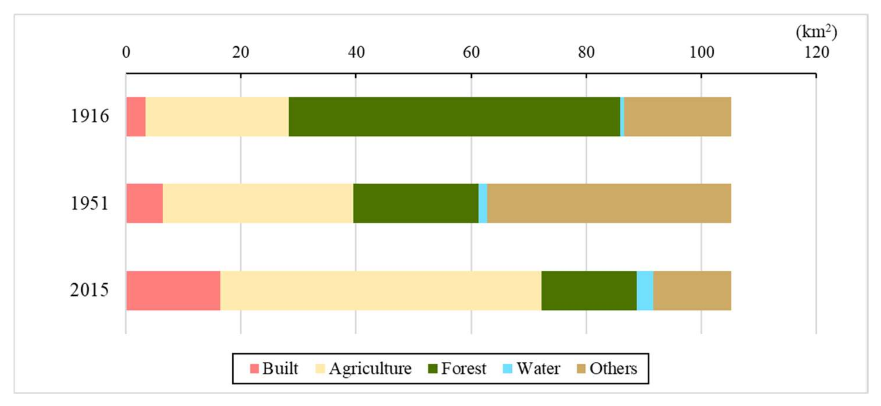
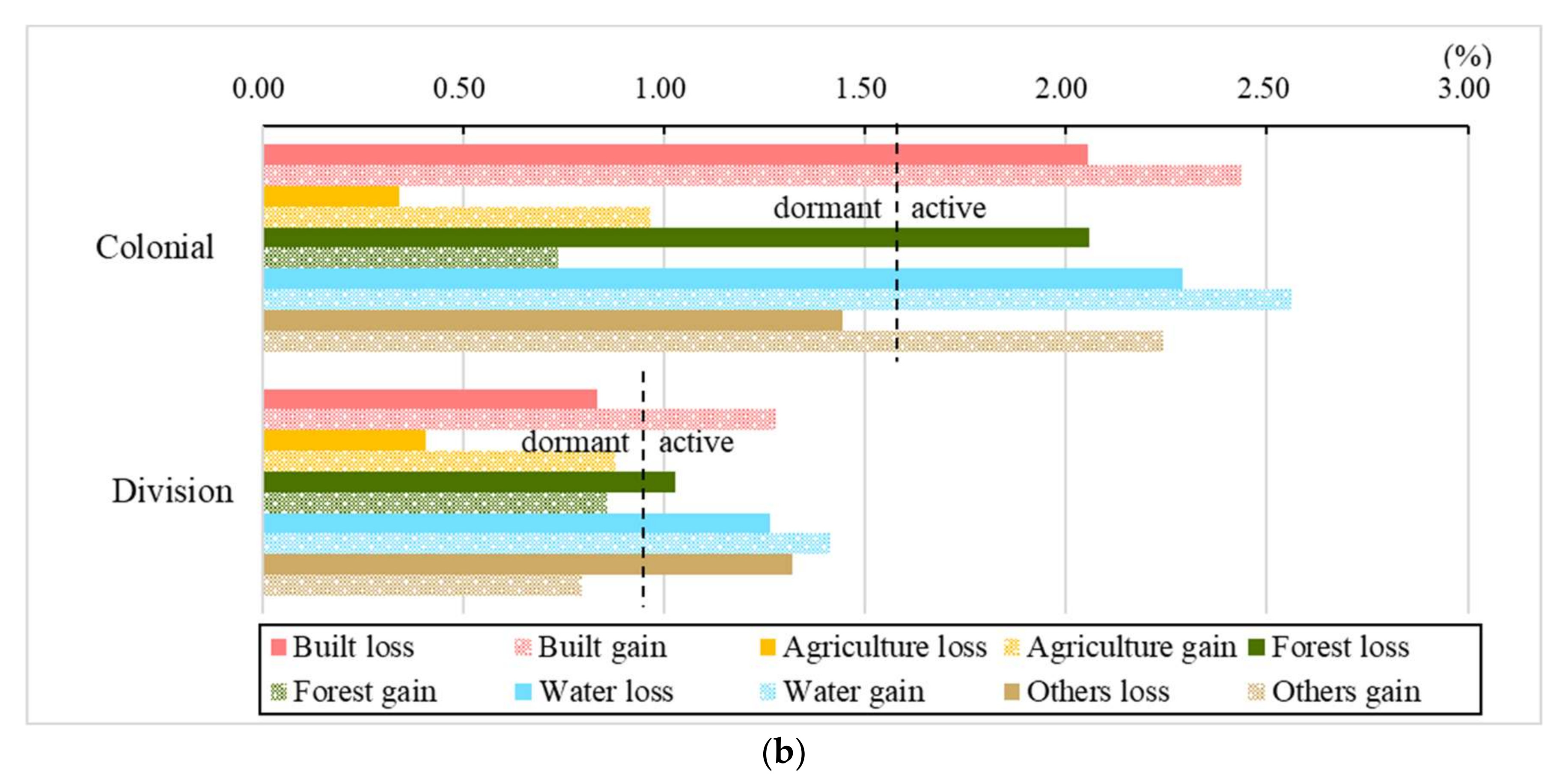
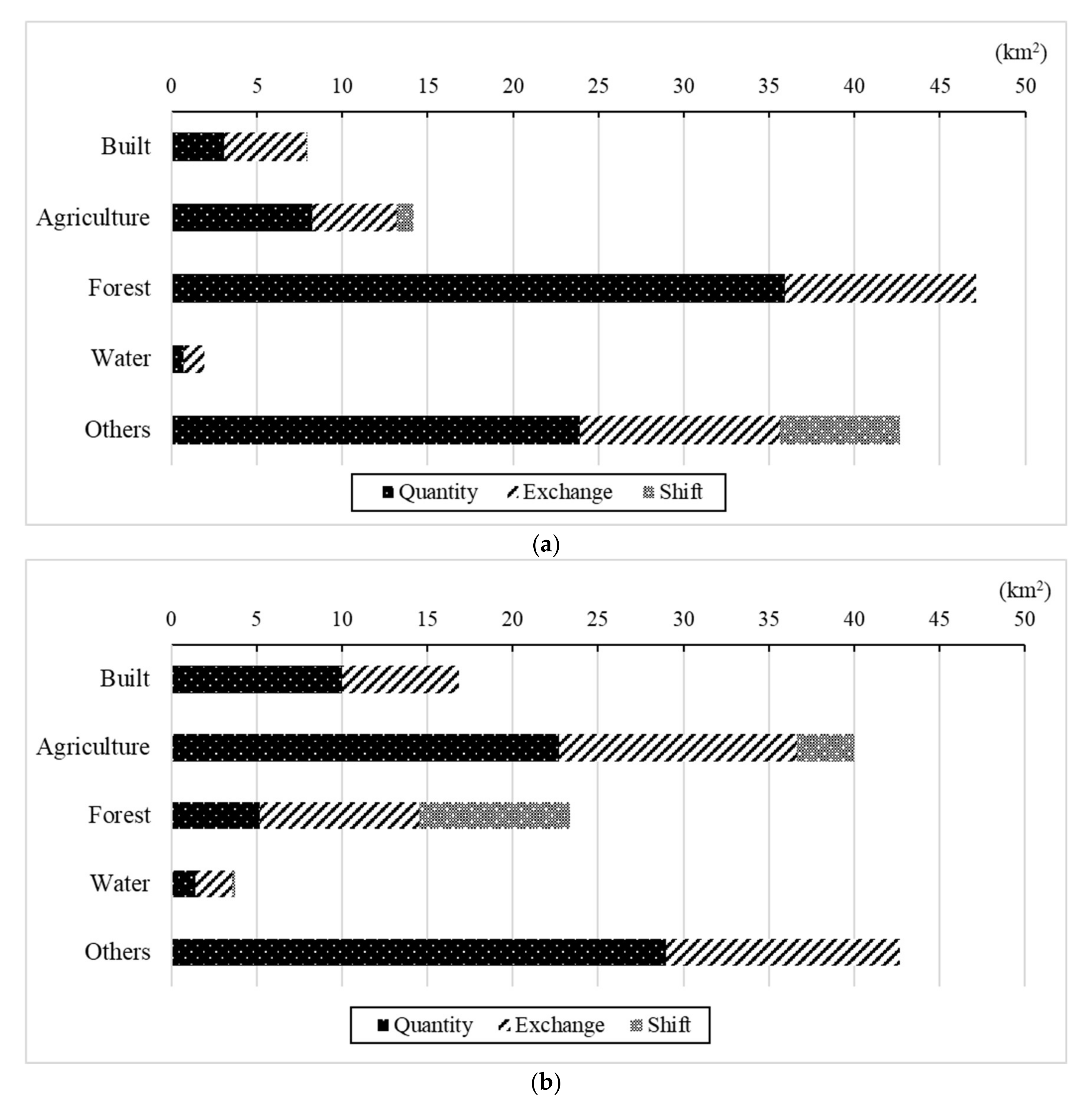
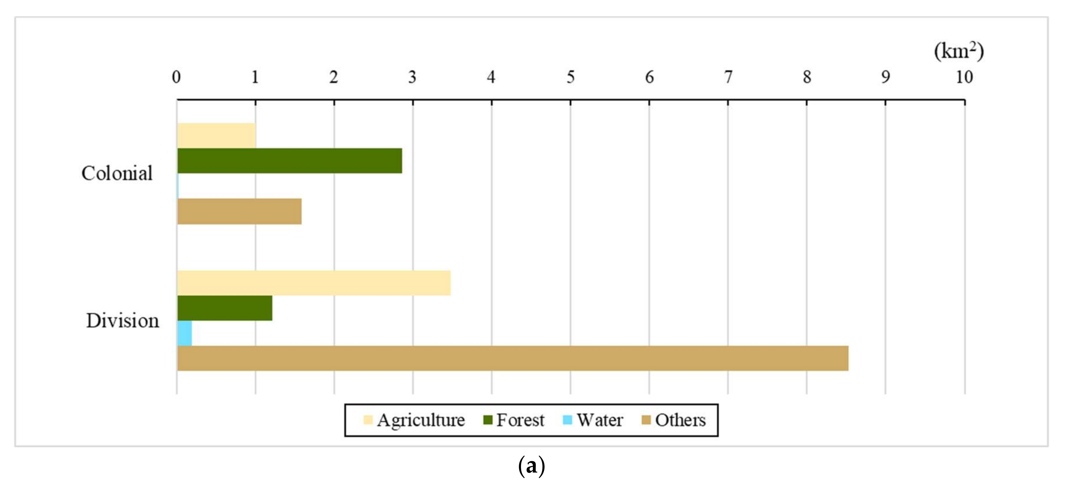
Figure 1. Geographical location of multiple study areas from the existing literature regarding the DMZ (upper-right) and our study area: the location of Kaesong and the adjacent DMZ area (bottom). The study area (black-dashed rectangle) is situated on the western side of the peninsula. Both the MDL and DMZ were determined by the Armistice Agreement in 1953 and digitized here based on this pact [22]. Notably, locational error exists in the background map provided by ArcGIS, as Panmunjom is incorrectly mapped in the middle of the river stream within the Kaesong region. In reality, Panmunjom is situated to the east, outside the present study area, in the middle of the MDL along a road connecting South and North Korea.
Land 11 00357 g001
Figure 2. Land-cover maps in: (a) 1916 (p57), (b) 1951 (p59), and (c) 2015 (p61) [18].
Land 11 00357 g002aLand 11 00357 g002b
Figure 3. Conceptual diagram of methodology for the analysis of three intensity levels and change components.
Land 11 00357 g003
Figure 4. Land area by category in 1916, 1951, and 2015.
Land 11 00357 g004
Figure 5. Change detection analyses: land-use and land-cover (a,c) gains and (b,d) losses under the colonial and division periods, respectively.
Land 11 00357 g005aLand 11 00357 g005bLand 11 00357 g005c
Figure 6. Interval level rates of change: (a) rate of change in each period and (b) annual rate of change (i.e., intensity).
Land 11 00357 g006
Figure 7. Interval level change (divided into Quantity, Exchange, and Shift) with respect to: (a) area, (b) intensity, and (c) Overall.
Land 11 00357 g007aLand 11 00357 g007b
Figure 8. Category level losses and gains by: (a) area and (b) intensity.
Land 11 00357 g008aLand 11 00357 g008b
Figure 9. Category level change components in area during: (a) the colonial and (b) the division periods.
Land 11 00357 g009
Figure 10. Category level change components in intensity during: (a) the colonial and (b) the division periods.
Land 11 00357 g010
Figure 11. Transition level changes: (a) To Built (area), (b) To Built (intensity), (c) To Agriculture (area), (d) To Agriculture (intensity), (e) To Forest (area). (f) To Forest (intensity), (g) To Water (area), (h) To Water (intensity), (i) To Others (area), and (j) To Others (intensity).
Land 11 00357 g011aLand 11 00357 g011bLand 11 00357 g011cLand 11 00357 g011d
Table 1. Crosstabulation of land-use and land-cover changes (LUCCs) in square kilometers during: (a) the colonial period (1916–1951) and (b) the division (1951–2015).
Category at Beginning of PeriodCategory at End of PeriodInitial
Total
Gross
Loss
BuiltAgricultureForestWaterOthers
(a)
Colonial period
(1916–1951)
Built0.950.720.160.031.513.372.42
Agriculture1.0021.931.510.430.0424.912.98
Forest2.866.8416.110.4131.3957.6141.51
Water0.020.220.000.150.360.750.60
Others1.593.433.930.419.1518.519.36
Final total6.4233.1421.711.4442.45105.1656.87
Gross gain5.4811.215.601.2933.2956.870.00
(b)
Division
(1951–2015)
Built3.002.550.240.090.556.423.43
Agriculture3.4824.490.981.512.6933.148.65
Forest1.219.537.450.083.4421.7114.26
Water0.200.750.040.270.181.441.16
Others8.5318.557.830.926.6242.4535.83
Final total16.4155.8716.532.8813.47105.1663.33
Gross gain13.4231.389.082.606.8563.330.00
Table 2. Uniform intensities at the interval, category, and transition levels.
LevelPeriodUniform Intensity (%)
Interval level-1.25
Category levelColonial1.55
Division0.94
Transition levelTo BuiltColonial0.15
Division0.21
To AgricultureColonial0.4
Division0.68
To ForestColonial0.34
Division0.17
To WaterColonial0.04
Division0.04
To OthersColonial1.1
Division0.17
Table 3. Change component intensities and their Overall values.
Land CategoryQuantityExchangeShift
Colonial
(1916–1951)
Built0.390.610.00
Agriculture0.580.350.07
Forest0.760.240.00
Water0.360.640.00
Others0.560.270.17
Overall0.530.420.05
Division
(1951–2015)
Built0.590.410.00
Agriculture0.570.350.08
Forest0.220.400.38
Water0.380.560.06
Others0.680.320.00
Overall0.490.410.10
Publisher’s Note: MDPI stays neutral with regard to jurisdictional claims in published maps and institutional affiliations.

