Spatial and Temporal Dynamics of Wetlands in Guangdong-Hong Kong-Macao Greater Bay Area from 1976 to 2019

Abstract

Wetland ecosystems contain rich natural resources and vital ecological functions, and the investigation of spatial and temporal evolution characteristics of wetlands and their driving factors is critical for the management and conservation of wetlands. This study aimed to explore the spatial and temporal dynamics of wetlands in the Guangdong–Hong Kong–Macao Greater Bay Area (GBA) from 1976 to 2019 using multi-source remote sensing data (DISP KH-9, Landsat, and GaoFen-1), combing with the object-based classification method and landscape invasion index, and further analyze the driving forces affecting the spatial and temporal evolution of wetlands. The results showed that: (1) The total area of wetlands in the GBA showed a trend to first increase and then stabilize from 1976 to 2019. (2) The rapid development of aquaculture led to a continuous increase in aquaculture ponds and offshore aquaculture and a flat change in the middle and late stages, the area of mangroves declined substantially before 2000 and has gradually recovered since then, the invasion of various types of wetlands by built-up land is increasing, and wetlands are becoming increasingly fragmented. (3) The wetland changes in the GBA are the result of a combination of natural factors and human activities. Environmental conditions represent the basis for wetland dynamics, while the population, socio-economics, and policies are important drivers of wetland evolution. The findings will be beneficial to the understanding of wetland dynamic changes in the GBA over the past 40 years, and helpful to the scientific management and sustainable development of wetlands.

1. Introduction

Wetland ecosystems are rich in natural resources and have great ecological service values. The international definition of wetlands is not yet unified, but the concept mentioned in the Convention on Wetlands is more commonly used, specifically natural or artificial, permanent or temporary, stagnant or flowing water, fresh, brackish, or salt-water marsh, peatland, or water, including areas of sea water not exceeding 6m in depth at low tide [1]. Wetlands have the reputation of being the kidneys of the earth and play an important role in providing marine resources, purifying water and gas, controlling pollution, sequestering carbon and releasing oxygen, and regulating global climate [2], and they also have high economic, scientific, and educational values. However, as the negative impacts of global environmental change and human activities intensify, wetland ecosystems are suffering serious impacts [3]. The degradation of wetlands is mainly manifested by the rapid reduction of wetland areas, changes in landscape patterns, species extinction, and reduction of ecological service functions, which are increasingly serious [4]. The monitoring of spatial and temporal dynamics of wetlands and the analysis of driving mechanisms of wetland changes, including natural factors and anthropogenic disturbances, can help to provide decision support for the protection and management of wetlands.

Remote sensing technology has the advantages of wide observation range and strong temporal periodicity, which has been widely used in land use/land cover change (LUCC) studies [5,6,7]. It has an important position and efficient advantage in dynamically monitoring the spatial and temporal evolution of wetlands on a large scale and over a long period of time [8,9,10]. Geographic information system (GIS) technology has the function of spatial data management and spatial analysis, which can accurately and efficiently manage, count, evaluate and analyze the changes of wetland resources. The combination of remote sensing and GIS has become an effective method for studying the dynamic evolution of landscape patterns, revealing spatial and temporal patterns of change, and exploring the drivers of evolution [11]. The use of remote sensing and GIS to investigate wetland ecosystems has been used for a long time [12]. In the 1980s, color infrared images were applied to monitor coastal wetlands in Delaware to illustrate the negative effects of human activities on wetlands [13]. The relationships between spectra and biomass of coastal wetland vegetation were explored with the Landsat-MSS images [14]. Subsequently, the high spatial resolution images [15] and radar images [16] are used for the analysis of dynamic changes in wetland landscapes and wetland classification. To date, with the development of remote sensing technology, there are abundant and diverse data sources have been used to explore various aspects of wetland ecosystems [17,18,19,20], including the changes of wetland landscapes [21,22], the drivers of wetland spatiotemporal evolution [23,24], functions and responses of wetland ecosystem services [25,26], wetland types classification [27,28], functions and environmental benefits of wetland ecosystems [29,30,31,32], impacts of wetland landscapes on biodiversity [33,34], and climate changes [35] etc. In terms of data sources, time-series wetlands were generally extracted based on 3–5 phase remote sensing images [36]. Among them, the medium resolution Landsat images are widely used in wetland studies at global and regional scales [37], while the high spatial resolution images, such as SPOT, ALOS, IKONOS, WorldView, and Quickbird, were used for local-scale wetland studies [38,39,40]. In addition, the extraction of wetland spatial distribution was obtained using auxiliary information, such as topography and statistical data.

The Guangdong–Hong Kong–Macao Greater Bay Area (GBA) is one of the most economically developed, open, and densely populated city clusters in China [41,42]. Wetlands are one of the most important ecological resources of the GBA, while the rapid development of the GBA has made regional ecological safety a great challenge. Existing studies mostly focused on natural wetlands, such as mangrove forests, while the knowledge of spatial and temporal changes of wetlands in the GBA is still insufficient. Therefore, it is necessary to monitor the wetlands in the GBA over a long time series and explore their change patterns and driving forces.

This study explored the temporal and spatial evolution characteristics of wetlands in the GBA based on the KH, Landsat, and GaoFen-1 images from 1976 to 2019, using the object-based classification and visual interpretation, and discussed the impact of including natural environment, population and economy, and government policy in GBA on wetland changes. The objective of this research is to (1) analyze the spatial and temporal change patterns of wetlands using land use dynamic degree, land use transfer matrix, and landscape invasion index; (2) investigate the transformation relationship between various types of wetlands, especially wetlands invaded by built-up land; (3) reveal the driving forces affecting wetland dynamics in the GBA.

2. Materials and Methods

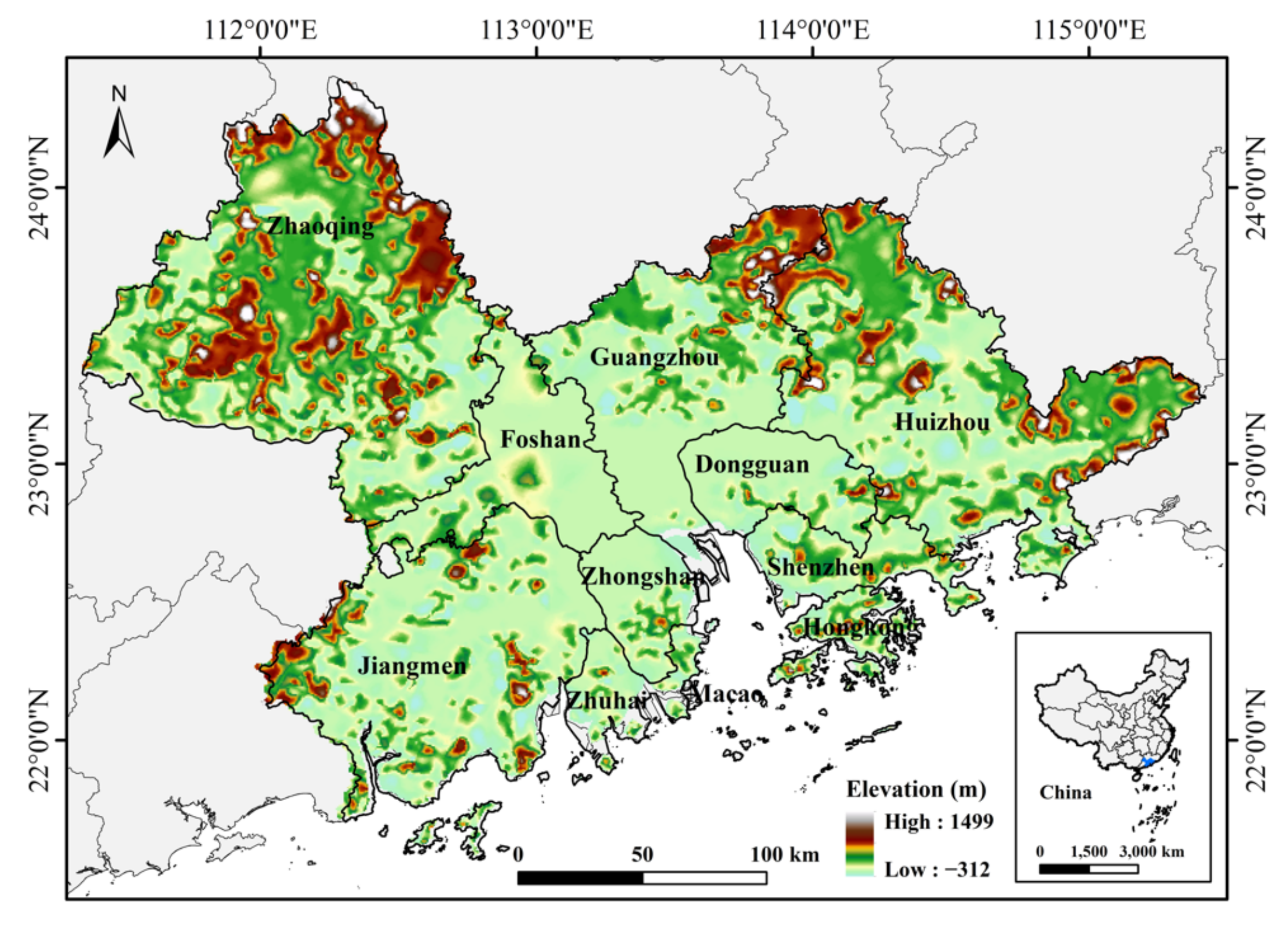
2.1. Study Area

The Guangdong–Hong Kong–Macao Greater Bay Area (GBA) of China (21°34′2″ N–24°23′30″ N, 111°21′24″ E–115°25′18″ E) was selected as the study area (Figure 1). The GBA includes the cities of Guangzhou, Shenzhen, Zhuhai, Foshan, Huizhou, Dongguan, Zhongshan, Jiangmen, and Zhaoqing in Guangdong Province, plus Hong Kong and Macau. With an area of 56,000 km² and a total population of about 70 million by the end of 2017, the GBA is one of the most open and economically dynamic regions in Chin, and has an important strategic position in the overall development of China [8,43,44]. The climate is a subtropical monsoon climate, warm and humid all year round, with precipitation mainly concentrated in April–September. The topography is mainly hilly plains, with low and gentle undulations. The east, north, and west are surrounded by mountains, hills, and terraces, and the central part of the country has an overall distribution of plains, interspersed with low and medium mountains, hills, and terraces. The GBA has a high density of river networks, with the Pearl River forming the main river delta, and a wide range of wetland types and distribution [42,43,45].

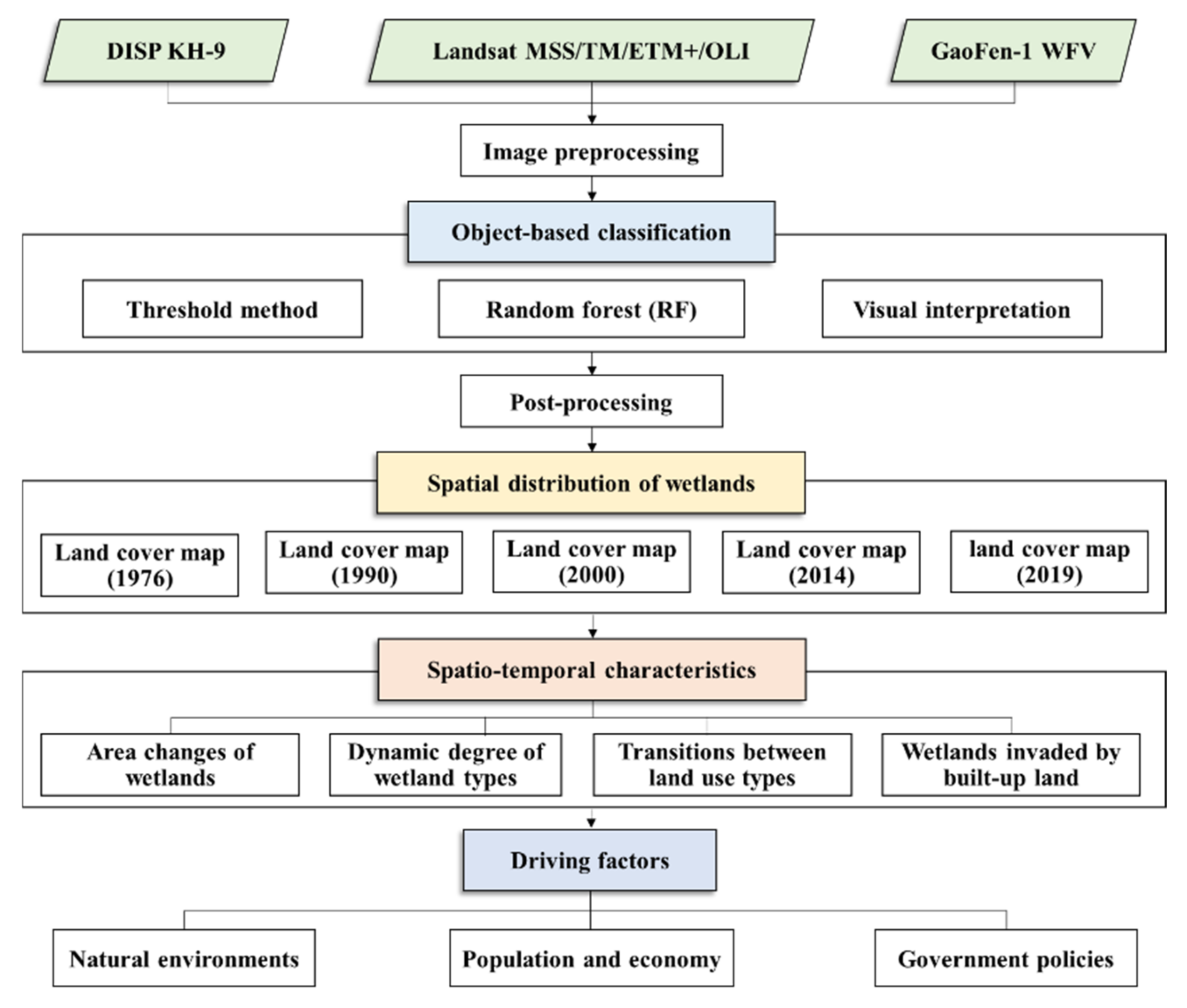
2.2. Data and Preprocessing

As show in

Table 1. Summary of remote sensing data used and pre-processing steps taken in this study.

Satellite	Sensor	Acquisition Date	Spatial Resolution	Geometric Correction	Image Mosaic	Image Clipping	Image Fusion
DISP	KH-9	20-12-1973, 17-12-1975 11-01-1976, 18-01-1976	5 m after resampling	√ *	√	√	√
Landsat	MSS	24-01-1977, 12-01-1977 02-11-1978, 03-11-1978 30-09-1979, 18-10-1979 19-10-1979, 20-10-1979	78.5 m	√	√	√	√
Landsat	TM	06-07-1989, 19-10-1989 20-11-1989, 24-11-1988 10-12-1988, 06-05-1990 21-09-1990, 13-10-1990 22-10-1990, 23-12-1990 02-09-1991, 21-09-1991 09-10-1991	30 m	√	√	√	×
Landsat	ETM+	20-08-1999, 26-12-1999 15-11-1999, 24-12-1999 01-11-2000, 10-11-2000 22-12-2001, 29-12-2001 31-12-2001	30 m	√	√	√	×
Landsat	OLI	05-10-2013, 29-11-2013 31-12-2013, 16-01-2014 23-01-2014, 08-10-2014 15-10-2014, 16-11-2014 25-11-2014, 16-04-2015	30 m	√	√	√	×
GaoFen-1	WFV	25-01-2019, 02-12-2019 07-12-2019, 11-12-2019	16 m	√	√	√	×

Note: √ denotes the pre-processing was performed; × denotes the pre-processing was not performed; * denotes image rotation was performed before geometric correction.

, the remote sensing images employed in this study mainly include the US spy satellite KH-9 images (5 m after resampling), Landsat MSS images (78.5 m), Landsat TM/ETM+/OLI images (30 m), and GaoFen-1 images (16 m) with the time points of 1976, 1990, 2000, 2014, and 2019. The 1976 study image was obtained by fusing the 1976 KH-9 images with the 1978 Landsat images, the 1990, 2000, and 2014 images were obtained by stitching and cropping the Landsat data around the corresponding time points, and the 2019 images were obtained by stitching and cropping the GaoFen-1 images around 2019.

The corresponding pre-processing operations were performed in terms of different data sources. The Landsat images need to be combined into one file for each band. The KH image has an overall 90° counterclockwise rotation with respect to due north, thus the clockwise rotation 90° is required. The KH image is a central projection with certain geometric deformation and no projection coordinates. The geometric correction process unifies the image projection into an Albers equiprojected conic projection, and the coordinate system uses the WGS-84 coordinate system. The geometric correction takes the corrected 2000-era image as the reference, and then performs geometric correction on other remote sensing images in turn. Approximately 12 uniformly distributed control points are selected for each image, and the root-mean-square error is controlled within 0.2 pixels. The bilinear method is chosen to resample the output images, and finally image stitching and cropping are performed. The pre-1984 Landsat satellite was equipped with the MSS sensor, and its images had a spatial resolution of 78.5 m. To compensate for the lack of spatial resolution, in this study, the MSS data around 1978 and KH-9 data around 1976 are fused with images using the Brovey method to obtain high-resolution multispectral images, and the spatial resolution is resampled to output 5 m. Although the images of the two periods differ by 2–3 years, the fused images are dominated by high spatial resolution information because of the slow urban development and small land use changes in the GBA, so the period of 1976–1978 can be defined as 1976.

2.3. Classification

2.3.1. Classification System of Land Use Types

Considering the geography and ground object characteristics of the study area, the classification system can be divided into three broad categories, namely built-up land, wetlands, and vegetation. In this study, the broad categories of wetlands are subdivided into more specific categories. In 1999, the State Forestry Administration established a classification system for wetland surveys, which was divided into five categories and 28 species. Niu et al. [46] proposed a remote sensing-based wetland classification system that could be linked to the classification system of the Wetland Convention in their study of remote sensing mapping of wetlands across China. Then, in 2010, they proposed a modified classification system with 15 secondary types, taking into account various classification systems already established by other scholars and the operability of remote sensing classification [47]. Referring to existing studies and the land use situation of the study area, in this study, the land use types of our study area were classified into nine categories, including mangrove, tidal flat, river, floodplain wetland, lake, aquaculture pond, offshore aquaculture, built-up land, and other land cover types. A classification system for the actual wetland types in the GBA was developed, as shown in

Table 2. Description of the land use and cover classification system used in this study.

Categories	Description
Mangrove	Woody biomes consisting of evergreen shrubs or trees dominated by mangrove plants, or tidal marshes covered with vegetation such as reeds and salt marshes
Tidal flat	Also known as sandbank, shallow beaches formed by the siltation of sediments such as stones, gravel, and silt at the bottom substrate, or mud and sand beaches and sand islands alluvial to the estuarine system, also including artificial reclamation temporarily formed by polder
River	Rivers with long-term water runoff
Floodplain wetland	The beaches and central islands that are flooded by the river during the high water period and exposed during the low water period due to seasonal effects
Lake	Also known as reservoir, naturally formed perennial water area due to low-lying terrain, or large artificially constructed water storage area under specific terrain, including the shallows exposed at the edge of the lake during the low water period
Aquaculture pond	Artificially constructed ponds on land for the purpose of freshwater aquaculture
Offshore aquaculture	Artificially reclaimed waters along the coast for the purpose of mariculture
Built-up land	Lands used for urban and rural settlements, factories or transportation facilities
Other	Other land cover types, include farmland and forest, etc.

.

2.3.2. Classification Method and Accuracy Assessment

The object-based classification is a classic method that segments the image, which forms the multiple neighboring image elements with strong homogeneous information into homogeneous objects of different sizes, and uses the object containing more semantic information as the processing unit [48]. It makes full use of the spectrum, shape, spatial relationship, and texture characteristics of ground objects, and to a certain extent reduces the Influence of same object with different spectrum and foreign object with same spectrum on classification, as well as the phenomenon of spectral interaction, so it can effectively avoid salt-and-pepper phenomenon [27]. Among current machine learning methods, the random forest (RF) has been an effective method widely used for wetland classification and mapping [49,50,51,52,53]. Thus, in this study, the object-based RF method was used for wetland classification based on remote sensing images listed in Table 1. Based on field investigations, the interpretation signs are formulated for the identifiable characteristics in different source images (

Table 3. Image interpretation signs for different data sources used in this study.

Categories	KH-MSS (RGB: 432)	Landsat TM/ETM+/OLI (RGB: 543; 543; 654)	GaoFen-1 (RGB: 432)
Mangrove
Tidal flat/Sandbank
River
Floodplain wetland
Lake/Reservoir
Aquaculture pond
Offshore aquaculture
Built-up land

), and the wetland classifications of the study area are performed using eCognition 9.0 software (Trimble, Westminster, CO, USA).

Considering the segmentation scale affecting the information, such as the number and size of homogeneous objects, this study set the segmentation scale to 60 for images in 1976, 15 for images in 1990 and 2000, and 125 for images in 2014 and 2019, using repeated comparison tests. According to the characteristics and separability of each type, built-up land, various types of wetlands, and other categories were extracted. The classification process involves visual interpretation, the threshold method, and object-based RF classification, as well as manual post-processing.

In step 1, the built-up land was extracted by visual interpretation. Many built-up lands consisting of smaller rural settlements in the 1976 image can be directly visually discerned, but they are more difficult to identify and maintain consistency in the later phases of the image, so built-up lands from that year were extracted separately. Specifically, the built-up land in the 1990s was first extracted by visual discrimination and exported as thematic maps. This thematic map was used for checkerboard segmentation before image segmentation of the 2000 image, and then designated the segmented part type as built-up lands. After that, the corresponding scale was selected for the overall image segmentation, and on this basis, the built-up lands 2000 image were visually discriminated to increase or decrease the designated built-up lands. The classification process for the images of the subsequent periods was followed in this way.

In step 2, the normalized difference vegetation index (NDVI) was used for threshold classification of vegetation, such as woodland, farmland, etc. The formula of NDVI is as follows [54]:

$$NDVI=\frac{{\rho }_{NIR}-{\rho }_{Red}}{{\rho }_{NIR}+{\rho }_{Red}}$$

(1)

where ${\rho }_{NIR}$ and ${\rho }_{Red}$ denote the reflectance of near-infrared band and red band, separately.

In particular, mangroves cannot be well distinguished from terrestrial vegetation only using automatic classification or simple spectral index, when the spectral and topographic information is not sufficient. Thus, mangroves need to be modified by visual interpretation in the post-processing process.

In step 3, the RF method was used for the classification of wetlands. The training samples were selected based on field investigations and the image interpretation signs (Table 3). For the images of each period, there are 15–20 samples selected for each type of wetland in each city, except for coastal wetlands, which can be selected slightly less than 15 samples due to their small distribution area. Based on the selected samples, the RF model is trained, and the feature layers used include all bands, texture features corresponding to the objects, and shape indices. The specific setting parameters include depth as 0, active variables as 2, and max tree number as 300. The trained classifier is used to automatically classify unclassified objects, and finally the classification results are checked and manually corrected.

To evaluate the classification results, the accuracy assessment is performed using samples of various land use types, to obtain confusion matrices and calculate overall accuracy (OA) [55].

2.4. Analysis of Spatial and Temporal Changes

2.4.1. Dynamic Changes of Wetlands

This study used a single land use dynamic degree to measure the change over time for each type of wetland in the study area, which is calculated as follows [56,57]:

$$K=\frac{U_b-U_a}{U_a}\times \frac{1}{T}\times 100\%$$

(2)

where $U_a$ denotes the area of a certain type of land use at the beginning of the study time period, $U_b$ denotes the area of a certain type of land use at the end of the study time period, and $T$ denotes the length of the study. When the unit of $T$ is year, the value of $K$ indicates the average annual rate of change of that type of land use type in that study time period [58].

2.4.2. Land Use Transfer Matrix

This study used a land use transfer matrix to quantitatively describe the transfer relationships between the various wetland types in the study area and with other non-wetland categories, expressed as [59]:

$$A_{ij}=\left[\begin{array}{c}\begin{array}{llll}{A}_{11}& A_{12}& \cdots & A_{1n}\end{array}\\ \begin{array}{c}\begin{array}{llll}{A}_{21}& A_{22}& \cdots & A_{2n}\end{array}\end{array}\\ \begin{array}{c}\begin{array}{llll}\cdots & \cdots & \cdots & \cdots \end{array}\end{array}\\ \begin{array}{c}\begin{array}{llll}{A}_{n1}& A_{n2}& \cdots & A_{nn}\end{array}\end{array}\end{array}\right]$$

(3)

where $A_{ij}$ denotes the area of the conversion of land use type $i$ to land use type $j$ during the study time period and $n$ denotes the total number of land use types.

2.4.3. Landscape Invasion Index

Previous studies have used various expansion metrics for quantifying urban expansion, such as built-up density, landscape shape index, largest patch index, etc. [60]. However, for wetlands, which are not always expanding land use types, it is difficult to use the above indicators to measure their increase or decrease in change. Scholars also analyzed three spatial patterns of urban expansion, i.e., infill, edge, and enclave [61], and further proposed the landscape expansion index (LEI) to quantitatively describe the process of landscape expansion dynamic and the spatial distribution of landscape expansion types [62]. Although the LEI has been widely used for the description of spatial patterns and processes of built-up land expansion [63,64], it is still difficult to employ it in wetland types where the dynamics of landscape patterns are both increasing and decreasing. The expansion of built-up land is actually an expression of invasion on other land types. In this study, we combine a new landscape expansion index proposed by Wu et al. [65] and extend the definition and application of this index to establish the landscape invasion index ($LII$) for the case of a certain type of land invading another type of land. The $LII$ is used to describe the spatial pattern and extent to which a particular type of landscape is invaded by the expansion of other landscape types within a given phase, and the formula of $LII$ can be calculated as:

$$LI{I}_i=\frac{A_i-A_0}{A_i+A_0}$$

(4)

where $A_0$ denotes the original patch area, $A_i$ denotes the patch area of a certain type of landscape that is adjacent to the original patch that is being invaded, and $i$ denotes the invaded patch.

The value range of $LII$ is [−1,1]. When $A_0$ = 0, it means that there is no original patch adjacent to the invaded patch, then $LII$= 1, which is outlying invasion type, or enclave invasion type. When $A_i$ = 0, it means that there is no invasion of a certain type of landscape by the original patches, and $LII$= −1. When $LII$ is in the interval of (−1,1), the invasion type is adjacent invasion type or edge-invasion type. The larger the value of $LII$, the larger the area of invaded patches relative to the area of original patches, which means a more intense degree of invasion.

Referring to the area weighted dike-pond invasion index (AWDII) [9], in this study, the area weighted landscape invasion index ($AWLII$) is proposed and calculated on the basis of $LII$:

$$AWLII={\displaystyle \sum }_{i=1}^n\left(LI{I}_i\times \frac{a_i}{A}\right)$$

(5)

where $LI{I}_i$ denotes the $LII$ of the invaded patch $i$, $n$ denotes the number of all patches in the invaded landscape type, $a_i$ denotes the area of the invaded patch $i$, and $A$ denotes the total invaded area of the invaded landscape type.

A larger $AWLII$ means that the landscape type is more heavily invaded. In this study, built-up land was considered as the only active invasion type, the $LII$ and $AWLII$ were used to measure the extent of wetland invasion by built-up land.

Figure 2 illustrates the flowchart of the methodology. We analyzed the spatial and temporal dynamics of wetlands in the GBA from 1976 to 2019 based on multi-source remote sensing data using the object-based classification method and explored the impact factors affecting wetland changes.

3. Results

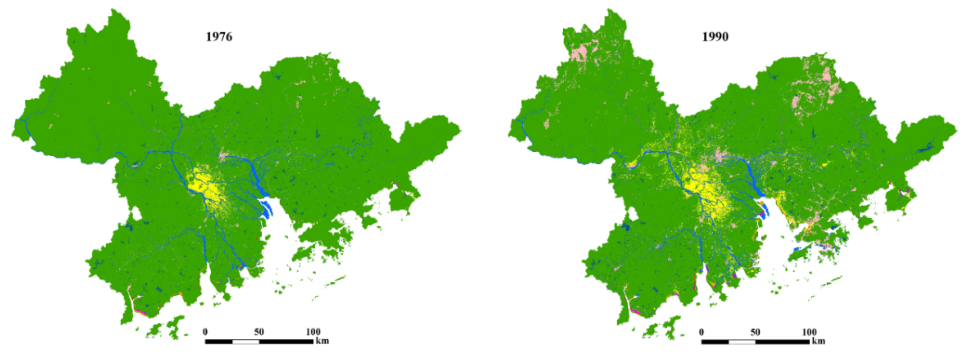
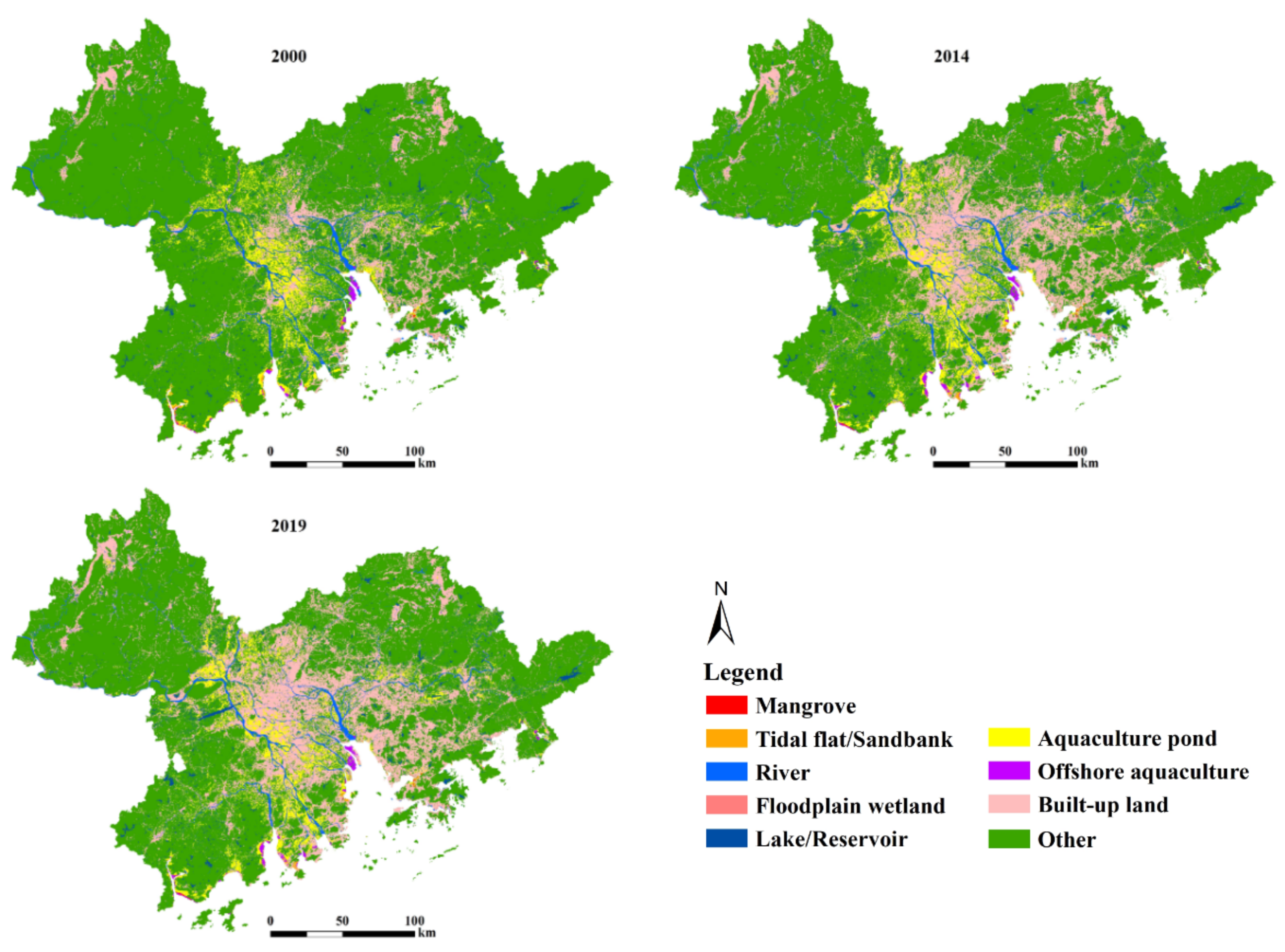
3.1. Spatial Distribution of Wetlands

The classification results of land cover types in the GBA from 1976 to 2019 are shown in Figure 3. The corresponding overall accuracy (OA) of the classification of land cover types in the GBA from 1976 to 2019 is listed in

Table 4. Overall accuracy of the land cover classifications in the GBA from 1976 to 2019.

Year	1976	1990	2000	2014	2019
Overall accuracy (%)	86.9	90.98	92.17	95.17	96.42

. Among these classification results for the five time periods from 1976 to 2019, the overall accuracy of 1976 reached 86.90%, which may be due to the low quality of the earlier image acquisition year, while the overall accuracies of the other years were all higher than 90%, with the highest overall accuracy in 2019, reaching 96.42%.

3.2. Spatial and Temporal Characteristics of Wetlands

3.2.1. Area Changes of Wetlands in the GBA

The total areas of each wetland type in the GBA from 1976 to 2019 and their proportion to the area of the GBA are listed in

Table 5. Area of each wetland type and the proportion of total area of the region.

Year	Category	Mangrove	Tidal Flat Sandbank	River	Floodplain Wetland	Lake Reservoir	Aquaculture Pond	Offshore Aquaculture	Total
1976	Area (km2)	21.00	73.07	1471.94	57.10	481.59	798.37	26.22	2929.30
	Proportion (%)	0.04	0.13	2.66	0.10	0.87	1.44	0.05	5.29
1990	Area (km2)	27.96	108.58	1598.87	120.75	755.83	1782.84	80.93	4475.76
	Proportion (%)	0.05	0.20	2.89	0.22	1.36	3.22	0.15	8.08
2000	Area (km2)	13.20	115.84	1386.34	89.20	751.03	2719.57	141.11	5216.29
	Proportion (%)	0.02	0.21	2.50	0.16	1.36	4.91	0.25	9.42
2014	Area (km2)	20.51	54.86	1439.71	19.98	1025.16	2816.05	170.59	5546.85
	Proportion (%)	0.04	0.10	2.60	0.04	1.85	5.08	0.31	10.02
2019	Area (km2)	21.18	50.22	1448.99	22.49	1098.64	2687.13	161.64	5490.29
	Proportion (%)	0.04	0.09	2.62	0.04	1.98	4.85	0.29	9.91

, indicating a trend to first increase and then stabilize, and the change magnitude continued to become smaller. The total area of all wetlands increased the most from 1976 to 1990, with an increase of 1546.46 km^2, and the next largest increase from 1990 to 2000, with an increase of 740.53 km². The total area of all wetlands changed relatively steadily from 2000 to 2019, remaining above 5200 km², with slight fluctuations during the period. Specifically, among various types of wetlands, mangroves and rivers have less variation and both remain slightly fluctuating within a certain level. Mangroves accounted for the smallest proportion of the various types of wetlands, accounting for less than 0.1% of the study area in all years. Rivers accounted for a relatively large proportion, between 2.5% and 3% of the study area, second only to aquaculture pond. The area change characteristics of aquaculture ponds were similar to the total area of all wetlands, with a trend of growth followed by stability. Aquaculture ponds continued to grow at a relatively large rate from 1976 to 2000, with an increase of more than 900 km² in the two study periods, while the change was stable from 2000 to 2019. Offshore aquaculture showed a continuous and large increase in area from 1976–2014 and a flat change in area from 2014 to 2019. Lakes/reservoirs had large increases in two time periods, 1976–1990 and 2000–2014, and relatively small changes in other time periods. Both floodplain wetlands and tidal flats/sandbanks account for a relatively small proportion of all types of wetlands, but there are large fluctuations, both showing an increasing trend followed by a decreasing trend. Floodplain wetlands reached a maximum of 120.75 km² in 1990, continued to decrease from 1900 to 2014, and rebounded slightly from 2014 to 2019. Tidal flats/sandbanks are formed under natural sediment accumulation on the one hand, and as intermediate wetlands transformed into other land uses under artificial reclamation activities on the other hand, so their area increases first and then decreases. Tidal flats/sandbanks increased significantly in two periods of 1976–1990 and 1990–2000, from 73.07 km² to 115.84 km², and then began to decrease significantly, indicating that the process of land formation during reclamation activities mainly occurred after 2000.

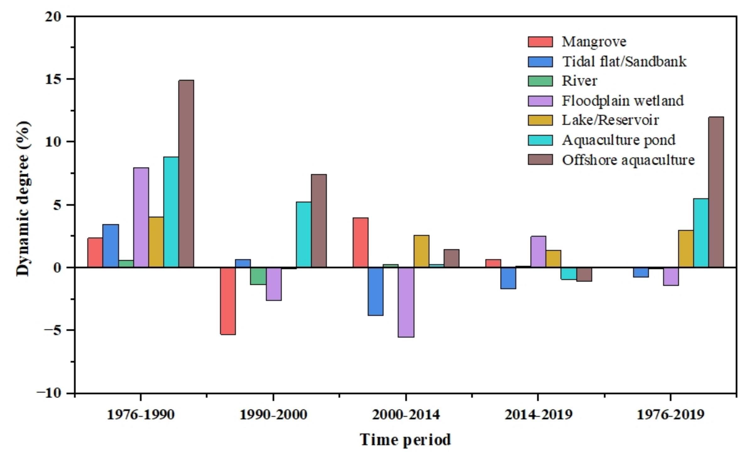
3.2.2. Dynamic Changes of Wetland Types

Figure 4 shows the land use dynamic degree of various wetland types in the study area calculated for the five time periods 1976–1990, 1990–2000, 2000–2014, 2014–2019, and 1976–2019. This gives the average annual rate of change for each type of wetland, with positive values indicating an increase in area for that time period and negative values indicating a decrease in area for that time period.

The land use type with most fluctuating dynamic degree among all wetland types is offshore aquaculture, followed by fishponds, both of which have the largest values of dynamic degree in the period of 1976–1990, and then gradually decrease and become negative in the fourth period. This indicates that the fishery develops rapidly at the beginning of the study period, growth becomes relatively difficult after reaching a certain area in the middle period, and the area of freshwater and marine aquaculture approaches saturation in the later period with insignificant dynamic changes. The river is the wetland type with the least dynamic fluctuations, and the absolute value of the dynamic degree does not exceed 1.4% for all time periods. The river is relatively stable and does not increase or decrease drastically in a short period of time, and its total area dynamics are slightly affected by changes in water volume upstream and downstream due to abundant and dry periods, or the construction of reservoirs. The dynamic degree of the lakes/reservoirs was relatively large in the periods of 1976–2014, which may be related to the artificial construction of reservoirs. As for mangroves, they have a negative dynamic degree in the period 1990–2000, which indicates that they were destroyed and their area was greatly reduced during this period. Their dynamic degree increased to 3.96% in 2000–2014, indicating that the mangroves recovered under artificial protection and suitable natural environment. In the period 2014–2019, their dynamic degree was relatively small and positive, indicating that they were well maintained during these years and did not suffer any further extensive damage. For the four time periods from 1976 to 2019, the dynamic degree of the tidal flat/sandbank is positive in the first two time periods, indicating an increase in area, and negative in the last two time periods, indicating a decrease in area. The tidal flats/sandbanks were initially dominated by natural tidal flats, and there was an overall increasing dynamic as new tidal flat wetlands were added due to increased artificial reclamation activities. Later, the reclamation activities decreased and some of the tidal flats were converted to land, so the overall flats/sandbanks decreased again.

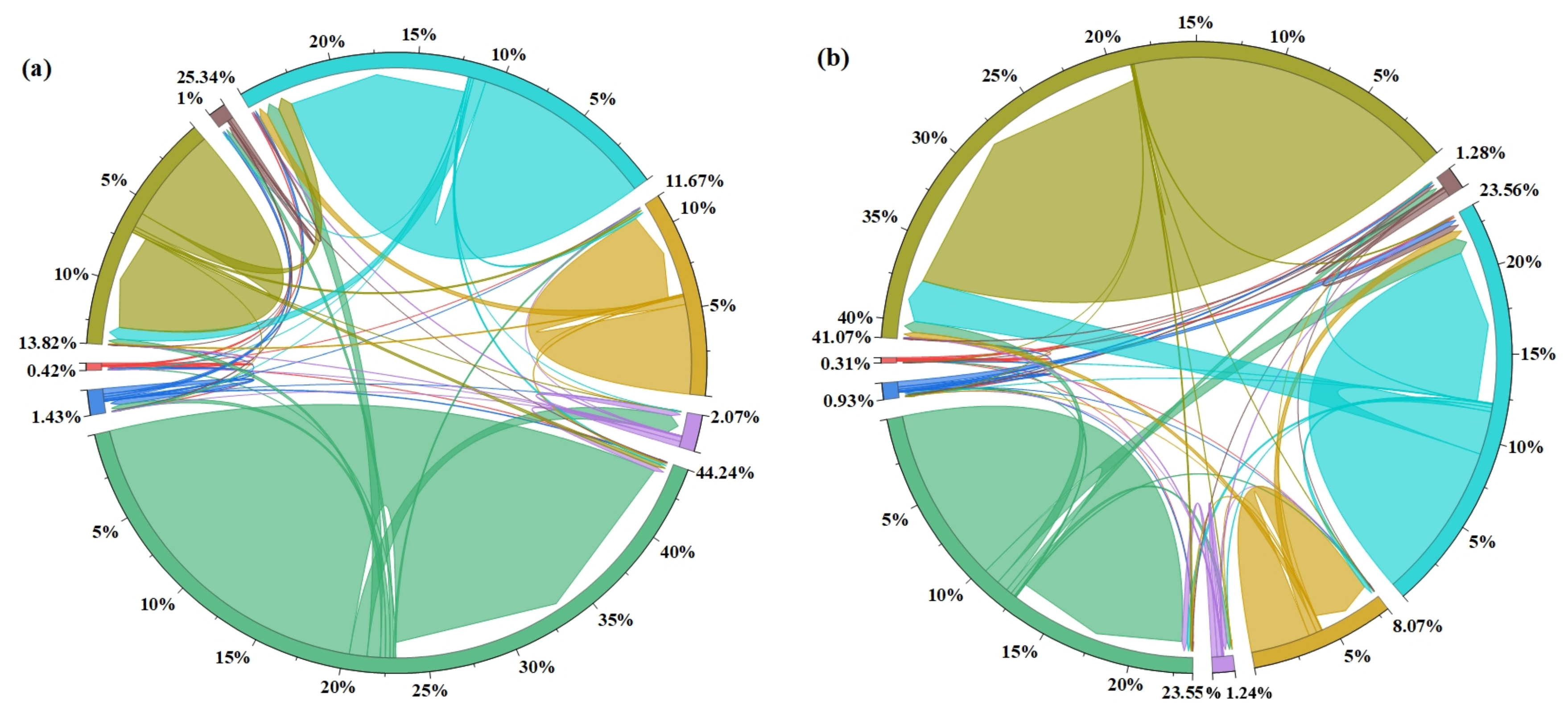
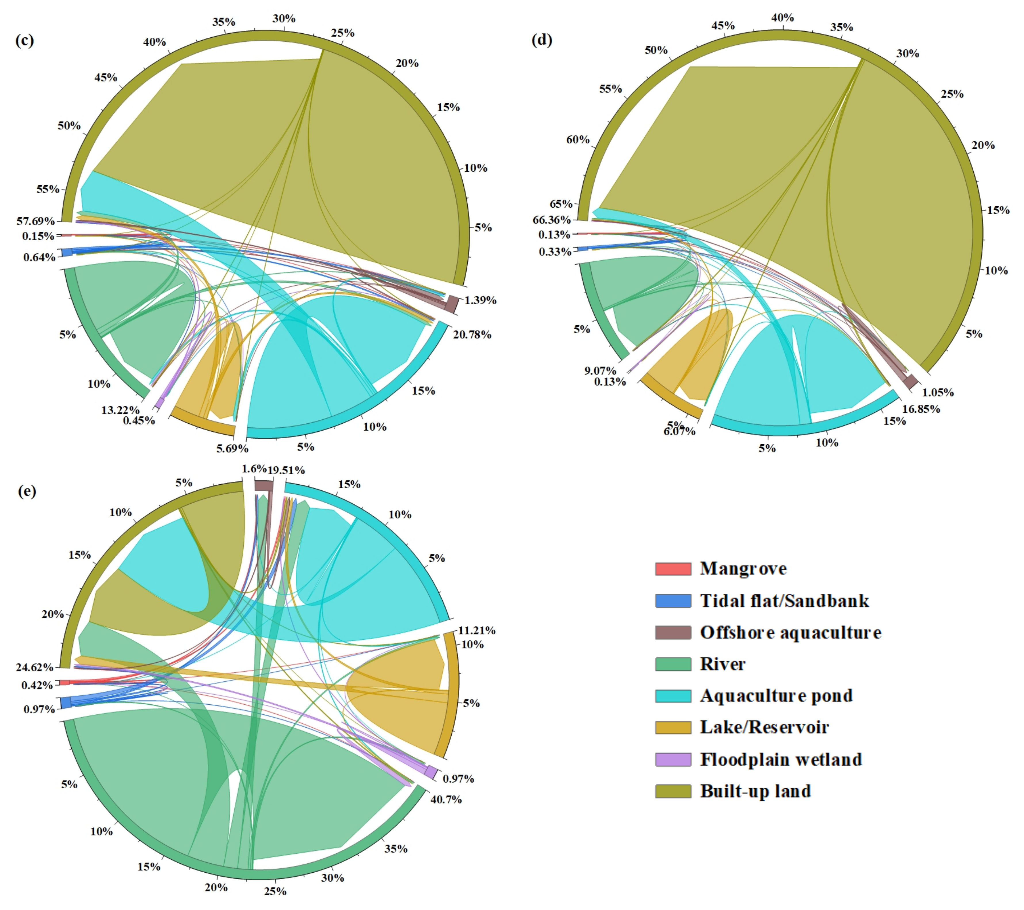
3.2.3. Land Use Transfer Matrix Analysis

This study used the land use transfer matrix and statistical analysis to quantify the transformation process of each land cover type, for five time periods, including 1976–1990, 1990–2000, 2000–2014, 2014–2019, and 1976–2019. Transitions between land use types in the GBA are illustrated in Figure 5 (corresponding to

Table A1. Area transfer matrix of each land cover type in the GBA from 1976 to 1990 (km²).

	1990	Mangrove	Tidal Flat/ Sandbank	River	Floodplain Wetland	Lake/ Reservoir	Aquaculture Pond	Offshore Aquaculture	Built-Up Land	Other
1976
Mangrove		5.74	0.97	0.68	0.00	0.25	1.74	0.88	0.19	10.55
Tidal flat/Sandbank		4.37	16.69	2.47	0.01	0.31	6.71	8.01	0.35	34.15
River		0.81	14.17	1041.53	53.60	6.07	39.53	10.85	15.14	290.24
Floodplain wetland		0.01	0.01	13.79	16.58	0.49	2.51	0.00	0.75	22.96
Lake/Reservoir		0.00	0.00	3.72	0.74	271.26	24.06	0.00	3.37	178.45
Aquaculture pond		0.03	0.08	6.94	0.30	8.10	559.59	0.50	37.25	185.57
Offshore aquaculture		0.19	2.29	0.41	0.00	0.00	5.56	11.22	0.13	6.42
Built-up land		0.00	0.16	11.34	0.45	7.37	43.87	0.00	293.29	7.27
Other		16.81	74.21	518.01	49.06	461.98	1099.27	49.46	1702.68	48115.47

,

Table A2. Transfer matrix of each land cover type in the GBA from 1990 to 2000 (km²).

	2000	Mangrove	Tidal Flat/ Sandbank	River	Floodplain Wetland	Lake/ Reservoir	Aquaculture Pond	Offshore Aquaculture	Built-Up Land	Other
1990
Mangrove		6.64	3.78	0.27	0.00	0.16	8.61	2.11	1.32	5.07
Tidal flat/Sandbank		0.43	15.12	2.65	0.00	0.34	32.52	10.44	5.13	41.96
River		1.69	6.62	1094.10	24.47	5.68	101.92	34.45	72.21	257.74
Floodplain wetland		0.00	0.18	34.72	28.37	0.48	4.24	0.00	6.27	46.48
Lake/Reservoir		0.00	0.18	4.07	0.20	369.22	50.14	0.19	31.67	300.16
Aquaculture pond		1.41	0.72	19.93	2.57	25.08	973.79	3.53	268.36	487.46
Offshore aquaculture		0.09	5.45	1.46	0.00	0.25	35.72	20.49	1.58	15.90
Built-up land		0.11	0.08	9.03	1.66	2.16	6.07	0.00	1983.74	50.31
Other		2.82	83.71	220.12	31.93	347.67	1506.56	69.90	2576.98	44011.39

,

Table A3. Transfer matrix of each land cover type in the GBA from 2000 to 2014 (km²).

	2014	Mangrove	Tidal Flat/ Sandbank	River	Floodplain Wetland	Lake/ Reservoir	Aquaculture Pond	Offshore Aquaculture	Built-Up Land	Other
2000
Mangrove		6.13	0.19	0.72	0.00	0.00	2.47	0.64	0.46	2.58
Tidal flat/Sandbank		5.68	12.46	4.41	0.00	0.37	22.40	28.65	13.28	28.59
River		0.35	5.83	1099.07	5.62	3.76	56.23	5.30	81.74	128.43
Floodplain wetland		0.00	0.00	34.41	12.03	0.25	2.77	0.00	15.40	24.32
Lake/Reservoir		0.09	0.06	4.21	0.02	424.78	54.22	0.21	79.99	187.45
Aquaculture pond		3.82	4.94	36.54	0.01	55.77	1413.17	32.66	723.54	449.11
Offshore aquaculture		1.84	8.16	1.38	0.00	0.17	20.12	70.38	16.93	22.15
Built-up land		0.11	0.03	8.30	0.18	4.77	5.80	0.05	4865.32	62.69
Other		2.49	23.19	250.67	2.12	535.29	1238.85	32.70	4453.71	38677.45

,

Table A4. Transfer matrix of each land cover type in the GBA from 2014 to 2020 (km²).

	2019	Mangrove	Tidal Flat/ Sandbank	River	Floodplain Wetland	Lake/ Reservoir	Aquaculture Pond	Offshore Aquaculture	Built-Up Land	Other
2014
Mangrove		18.73	0.01	0.06	0.00	0.00	0.60	0.57	0.10	0.45
Tidal flat/Sandbank		0.73	43.34	0.42	0.00	0.01	0.14	0.15	8.51	1.56
River		0.07	0.55	1330.19	3.20	0.69	10.06	0.53	40.52	53.89
Floodplain wetland		0.00	0.00	0.75	17.41	0.00	0.00	0.00	0.87	0.95
Lake/Reservoir		0.00	0.01	0.78	0.00	886.79	3.69	0.00	31.86	102.03
Aquaculture pond		0.41	2.26	8.13	0.00	9.44	2365.48	0.95	299.85	129.54
Offshore aquaculture		0.31	1.22	0.20	0.00	0.00	0.39	150.07	13.77	4.62
Built-up land		0.09	0.56	27.35	0.24	20.60	46.50	0.99	9822.71	331.35
Other		0.86	2.28	81.11	1.64	181.10	260.26	8.38	1832.80	37214.34

and

Table A5. Transfer matrix of each land cover type in the GBA from 1976 to 2000 (km²).

	2019	Mangrove	Tidal Flat/ Sandbank	River	Floodplain Wetland	Lake/ Reservoir	Aquaculture Pond	Offshore Aquaculture	Built-Up Land	Other
1976
Mangrove		1.03	0.34	0.27	0.00	0.02	7.91	3.84	3.85	3.75
Tidal flat/Sandbank		4.93	1.77	1.01	0.00	0.09	24.24	8.05	9.36	23.63
River		0.46	3.62	961.83	10.06	11.91	73.16	54.97	193.92	162.01
Floodplain wetland		0.11	0.00	27.80	1.74	0.50	3.10	0.00	9.90	13.94
Lake/Reservoir		0.00	0.00	2.89	0.00	276.71	16.47	0.00	45.53	139.99
Aquaculture pond		0.20	0.00	4.33	0.02	4.47	247.56	1.07	454.15	86.57
Offshore aquaculture		0.02	0.00	0.00	0.00	0.00	14.54	2.66	3.02	5.98
Built-up land		0.00	0.00	5.89	0.01	1.95	10.13	0.00	330.99	14.79
Other		14.43	44.49	444.98	10.66	803.00	2290.01	91.04	11000.28	37388.07

) using a chord diagram, which allows the visual representation of the inter-relationships between data in a transfer matrix. These chord diagrams illustrate the land use transitions for different time periods.

Result showed that the conversion of built-up land to other land types is less, while the invasion of other land types by built-up land gradually increases along its expansion, among which the largest area of invasion belongs to aquaculture ponds, followed by rivers. The invasion of built-up land is spatially scattered. In the main urban area, it is mainly the invasion of aquaculture ponds and farmland, and the specific activities are urbanization and development. In the southernmost area near the sea, it is mainly the invasion of rivers and tidal flats, and the specific activities are land reclamation and wharf construction. In the northern area, it is mainly the invasion of forest land, and the specific activities may be mining and logging and other ecological destruction. The tidal flats/sandbanks are mainly transferred from the sea in the type of other as a result of natural sediment accumulation action and man-made reclamation. There are generally two types of reclamation activities. One is to enclose the sea to create ponds for mariculture, and the other is to reclaim the sea to build construction land such as wharves, so the direction of the tidal flat/sandbank transfer out is mainly aquaculture ponds, offshore aquaculture, and built-up land. During 1990–2000, the reclamation activities were more intense. Thus, more sea areas were converted into tidal flats/sandbanks, which were mainly converted into aquaculture ponds and offshore aquaculture, and partly formed into built-up land under the effect of land reclamation. After 2000, the reclamation activities weakened, the area of sea area converted to tidal flats/sandbanks decreased, and the area of tidal flats/sandbanks transferred out gradually decreased also. The mangroves are mainly turned out for aquaculture ponds and offshore aquaculture, while supplemented by some tidal flats and a small amount of aquaculture ponds and offshore aquaculture. It suffered great damage during 1990–2000 and was better restored and maintained during 2000–2019. There was interconversion between rivers and floodplain wetlands, with a greater number of conversions from the latter to the former, suggesting a wetland development towards the wetter type in the study area. The source of lakes/reservoirs is mainly forest land in the type of other, with more new reservoirs. Aquaculture ponds are a type of wetland that continues to grow in area, mainly converted from agricultural land in the type of other. Aquaculture ponds have interconversion with rivers, lakes/reservoirs, and offshore aquaculture, respectively, but their transfer out to the other three types of wetlands is much less than the transfer in of the other three types to aquaculture ponds, which is one reason why the area of aquaculture ponds keeps growing. Offshore aquaculture is mainly transferred from rivers in the sea or estuary, but also partly indirectly from tidal flats, and the main direction of its transfer out of wetlands is aquaculture ponds.

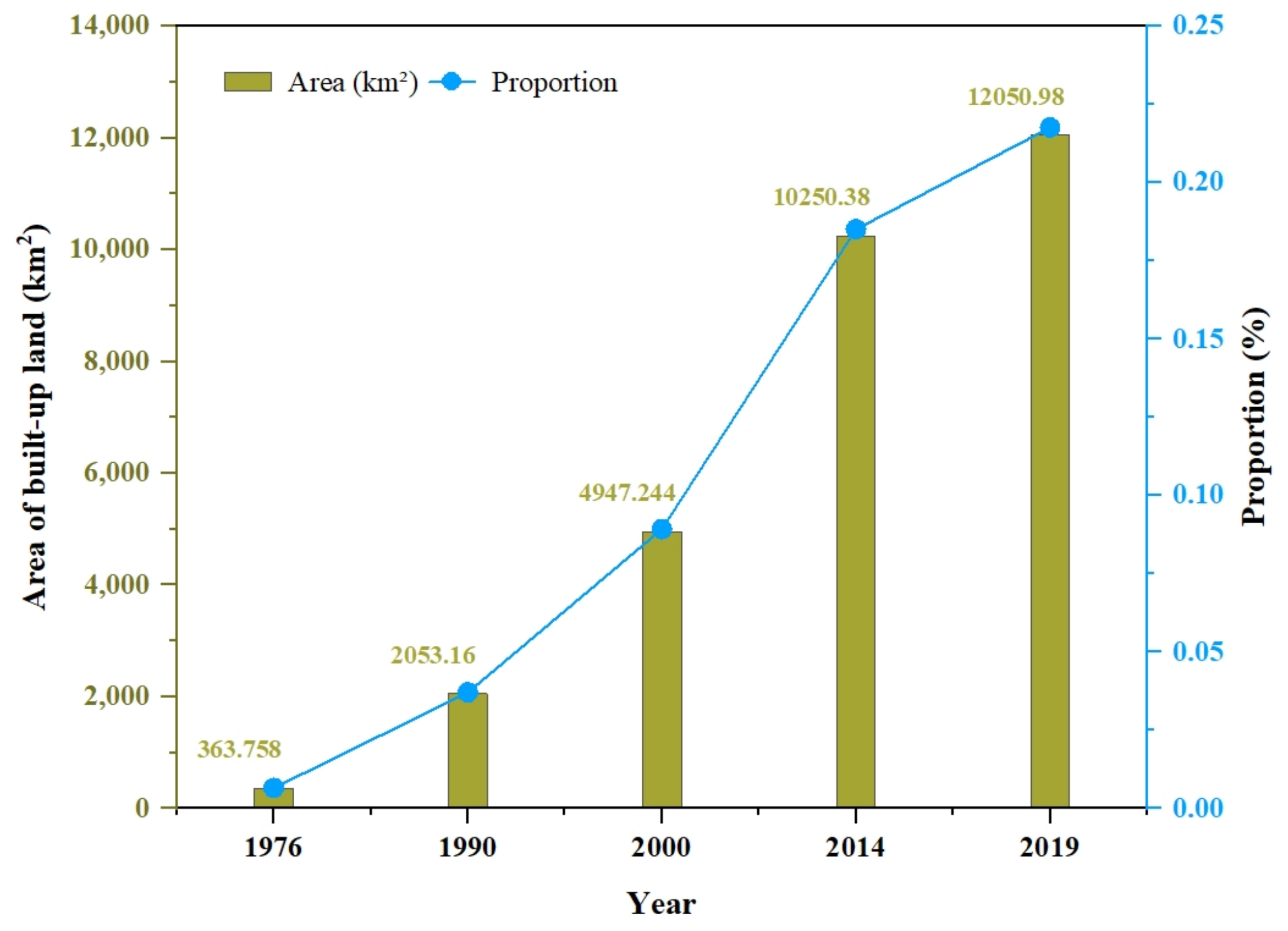
3.3. Analysis of Wetlands Invaded by Built-Up Land

As shown in Figure 6, the area of built-up land and its proportion to the area of the study area were calculated based on the classification results. It can be seen that the area of built-up land continues to expand rapidly, with the proportion of the area growing from 0.66% to 21.76%. The high growth of built-up land will inevitably take up other land types, resulting in a decrease in wetland area. To further analyze the encroachment of wetlands by built-up land, the area of wetlands invaded by built-up land was counted and the average annual encroachment area was calculated for four time periods of 1976–1990, 1990–2000, 2000–2014, and 2014–2019. In addition, the $LII$ of the invaded patches for each wetland type and the frequency of $LII$ occurrence in different intervals were calculated, as shown in Figure 7.

The $AWLII$ is calculated for each time period, as shown in Figure 8. The number of patches of wetlands invaded by built-up land during 1976–1990 was 4326, with a comparable proportion of enclave and adjacent invasion type, and the $AWLII$ of 0.275. During 1990–2000, the number of wetland invaded patches was 16,740, and enclave-type invasion was the main part in the number of patches in this period. The proportion of patches with LII values close to –1 increased, indicating that the invaded patches of small areas became more numerous. The $AWLII$ at this stage was 0.512, which increased compared to the previous time period, and the invaded area of wetlands and the average annual invaded area also increased compared to the previous time period, indicating that the invasion of wetlands by built-up land increased at this stage, and the enclave-type invaded area accounted for a larger proportion of the total invaded area. During 2000–2014, the number of wetland invaded patches was still dominated by enclave-type invasions. The $AWLII$ was 0.479, which was slightly reduced compared with the previous phase, but the invaded area of wetlands and the average annual invaded area increased significantly, indicating that the invasion of wetlands by built-up land was still increasing in this phase, but the proportion of adjacent invaded area increased among them, resulting in a smaller $AWLII$. During 2014–2019, adjacent type of invasion becomes dominant in terms of number of patches. The proportion of patches with $LII$ values close to –1 increased significantly, indicating a further increase in small area invasion and more fragmented wetlands. Compared with the previous phase, $AWLII$ decreased slightly to 0.452, and the average annual invasion area increased, indicating that the invasion of wetlands by built-up land was still increasing in this phase, and the proportion of adjacent invasion area increased. Overall, from 1976 to 2019, there is a steady expansion of built-up land and increasing invasion of wetlands. In terms of the number of patches, enclave type invasions were basically predominant before 2014 and adjacent type invasions were predominant after 2014. In terms of patch area, the proportion of adjacent invaded area has been increasing. The proportion of patches with $LII$ values close to –1 continues to increase, and wetlands are increasingly fragmented (Appendix A).

4. Discussion

4.1. Driving Factors of Wetland Changes

Over the past 40 years, the total area of wetlands in the GBA has continued to increase, with a large increase before 2000 and a more moderate change after 2000, plus an overall increase of nearly double. Main contributions include two types of artificial wetlands, i.e., aquaculture ponds and offshore aquaculture, which are mainly due to the reclamation activities [9]. The spatial and temporal evolution of wetlands in the GBA is recognized as the result of natural and human activities. Referring to previous studies and analysis of the statistical yearbooks, reports, and policies of the GBA, three main driving factors of wetland changes should be further analyzed, including natural environmental factors, population and economic factors, and government policies.

The natural environmental factors mainly include the topography, hydrology, and other natural conditions of the GBA, which are suitable for the development of beach wetlands and reclamation activities [66,67]. The Pearl River estuary carries a large amount of sediment, and the Baiteng sea-closure project in the late 1950s induced an overall reduction in the flow velocity of the Pearl River waters and further accelerated the deposition of downstream sediment, making tidal flat resources abundant and facilitating reclamation activities [67]. For example, a large amount of sediment from the upstream water system in the area of Nansha and Wanqingsha flows here with the river and is blocked and deposited by the peripheral islands to form sandbanks. In addition, the Modaomen estuary is a strong runoff, weak tide type estuary with rapidly developing tidal flats, making it easy for reclamation activities.

The rapid urbanization in the GBA has increased the demand for residential land, agricultural land, and industrial land, bringing about a boom in reclamation [66,68]. Studies have shown that the main way to relieve land supply pressure in China’s coastal cities is reclamation activities [66,69]. Figure 9 shows the number of resident population and gross domestic product (GDP) between 1990 and 2018 providing by the GBA City Cluster Yearbook. Both the resident population and GDP of the GBA have grown rapidly. By 2018, the GDP of the GBA was 810.4850 billion and the number of resident populations was 63.999 million, which were 80.49 times and 2.66 times of 1990, respectively. Rapid population growth has led to the expansion of urban scale, and high economic growth has been accompanied by a proliferation of various industrial parks, technology parks, and pioneer parks [67], which have placed demands on land supply and brought about a boom in reclamation. In addition, aquaculture plays an important role in the economic development of the GBA [9,70]. The coastal aquaculture and reclamation activities in the GBA have never ceased. Rather, they have become the main distributions of mulberry fishponds [67,70], which are the reason for the increasing number of both types of artificial wetlands, aquaculture ponds, and offshore aquaculture.

Government policies affecting the dynamics of wetlands can be divided into policies for promoting economic development and policies for protecting wetland ecosystem. The former focuses on economic development and urban construction, which to some extent increases the pressure on land in the GBA and leads to an increase in reclamation activities. The latter were enacted and implemented in response to the increasingly prominent ecological problems after the economic development of the city, aiming to promote rational development [66,67,71]. In 1978, China established the reform and opening-up policy and set up Shenzhen and Zhuhai as special economic zones. Shenzhen took advantage of its location to undertake the professional transfer from Hong Kong, and various port and road constructions sprang up [70]. Since then, China has implemented the policy of prioritizing the development of the eastern coastal areas and the policy of opening up coastal cities. In particular, from 1990 to 2000, Guangzhou, Shenzhen, Zhuhai, and other cities rapidly emerged with favorable policy conditions, and the coastal area of the Pearl River estuary became one of the most economically developed and urbanized regions in China [67]. This led to the dense population in the GBA and the scarcity of land for more people prompted reclamation activities to become a rapid boom [70].

4.2. Implications for Wetland Management

Given that the destruction and restoration of wetlands coexist due to anthropogenic interventions, it is necessary to analyze the changes in wetlands for smaller time intervals by using high spatial and temporal resolution imagery obtained by satellites launched in recent years, such as Sentinel-2 data. Moreover, wetland ecosystems are complex in composition and structure with high spatial and temporal heterogeneity and species diversity. Thus, further studies are required to further quantify and analyze the numerous drivers of wetland spatial and temporal evolution, especially in the rapid urbanization process.

Existing studies have focused on monitoring the changes of wetlands, grasping their spatial and temporal patterns, analyzing the causes of changes in wetland resources and their response to the natural factors and human activities [57,72], which are conducive to reconciling the relationship between urbanization and natural resource conservation. They also provide decision support for the rational development and protection of wetlands, and the development process of urbanization and the construction of ecological civilization.

As the rapid development of urbanization brings ecological and environmental problems [42], to achieve the sustainable development of the GBA, a series of relevant protection policies of wetlands are constantly being enacted and implemented. Since 2002, China has promulgated laws and regulations, reclamation activities have been significantly slowed down, and the artificial planting of mangroves has been started in several areas to protect coastal mangroves and tidal flats [66,73]. After 1975, a series of policies were implemented successively, imposing strict regulations on the scale of reclamation and marine protected areas. As a result, several nature reserves were established to further protect natural wetlands, such as the Mai Po Nature Reserve in Hong Kong, the Futian Mangrove Nature Reserve in Shenzhen, and the Qi’ao Island Mangrove Nature Reserve in Zhuhai [74,75].

5. Conclusions

This study explored the spatial and temporal change characteristics of wetlands in the Guangdong–Hong Kong–Macao Greater Bay Area (GBA) from 1976 to 2019 based on multi-source remote sensing data, investigated the transformation relationship between various land use types, especially the impacts of built-up land, and analyzed the driving factors of wetland changes, including natural environment, population, economy, and policies. The findings will provide a reference for decision making for government departments on the rational use of land resources and wetland conservation in the GBA, supporting the coordination of ecological conservation and regional development. The main conclusions are as follows:

(1)

The total area of wetlands in the GBA between 1976 and 2019 showed a trend of first growth and then stability, and the change magnitude continued to become smaller. Specifically, the aquaculture ponds and offshore aquaculture continued to increase at a relatively large rate in the first and middle stages, with flat changes in the later stages. Mangroves were greatly decreased in 1990–2000 and gradually recovered during 2000–2019 due to the artificial restoration planting.

(2)

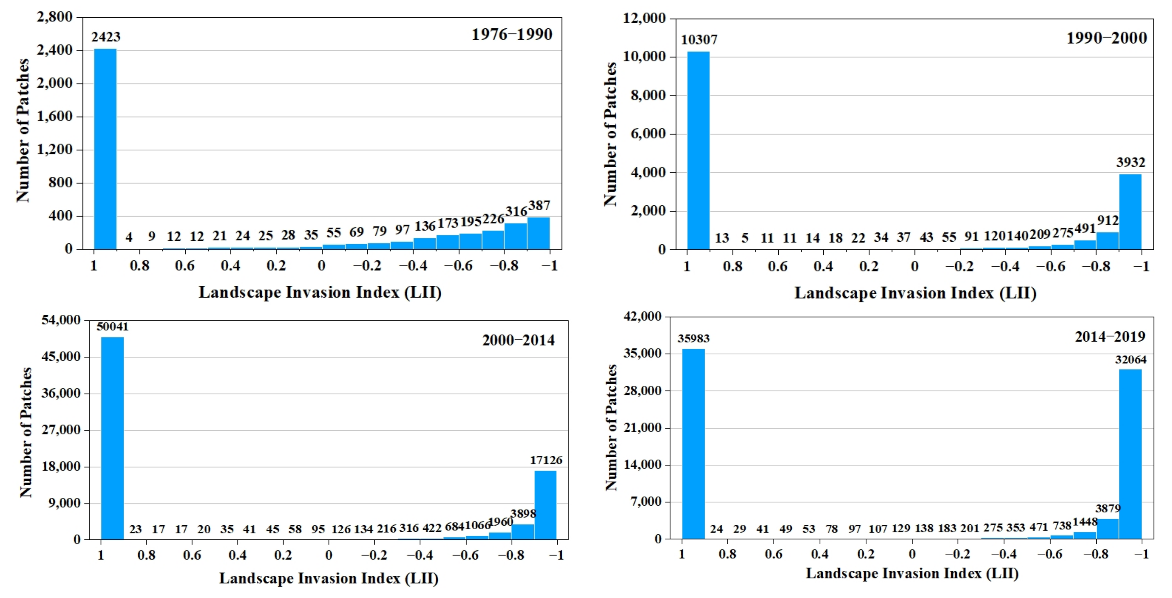
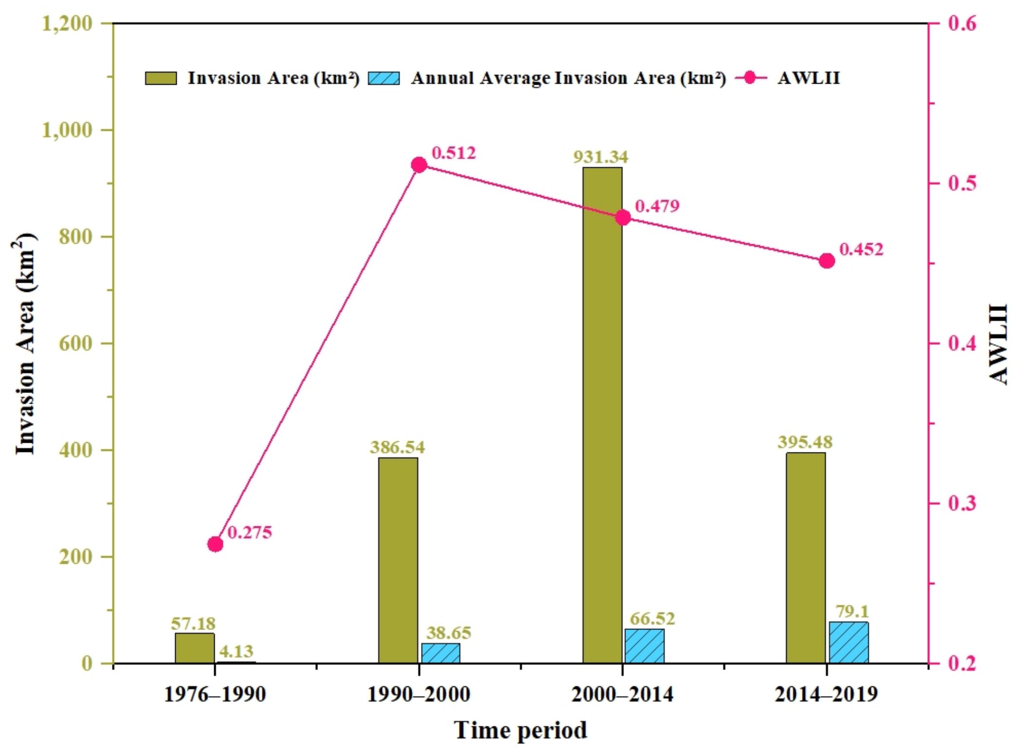
The area of wetlands encroached upon by built-up land continued to increase from 1976 to 2019. In terms of the patches of wetlands, the enclave invasions were basically dominant before 2014 and the adjacent invasions were dominant after 2014. The proportion of adjacent invaded area has been increasing. In addition, the wetlands of the GBA are increasingly fragmented with an increasing proportion of $LII$ values close to –1.

(3)

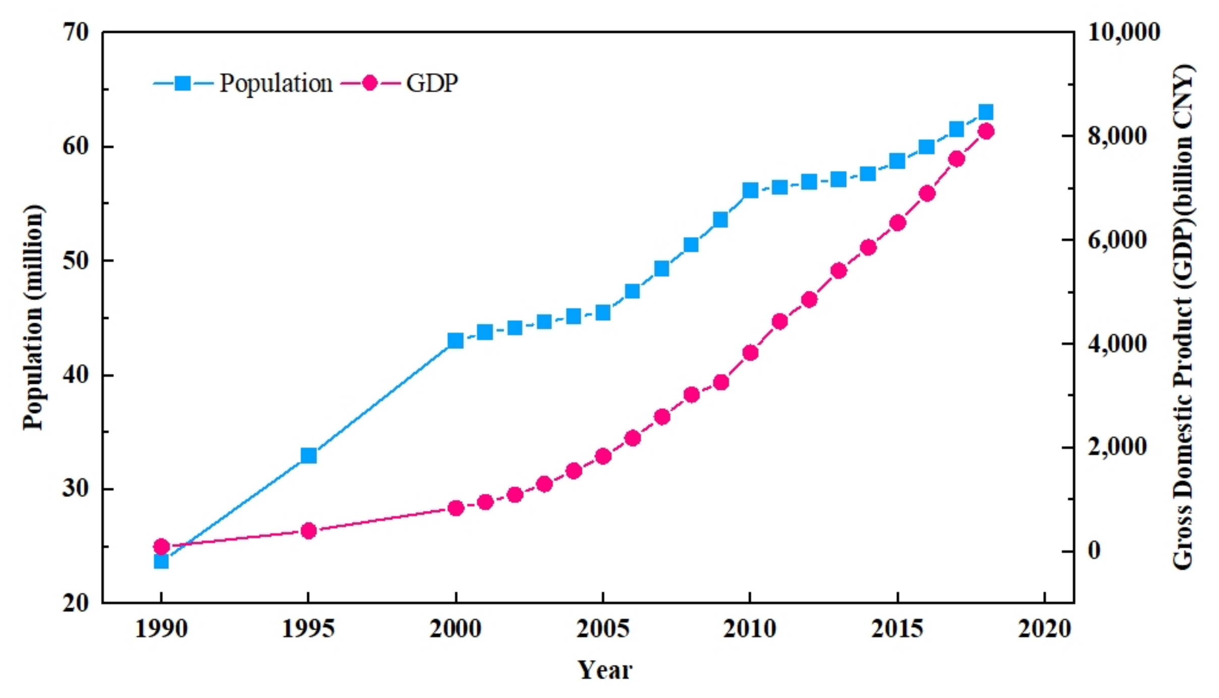
The spatial and temporal changes of wetlands in the GBA are mainly the result of both natural conditions and human activities. Environmental conditions, such as topography and hydrological characteristics, represent the basis of wetland evolution and one of the bases for facilitating reclamation. The population, socio-economics, and policies in the GBA are important drivers of wetland dynamics to consider in the promotion and constraint of reclamation activities.

References

1. He, Y.; Zhang, M.-X. Study on wetland loss and its reasons in China. Chin. Geogr. Sci. 2001, 11, 241–245. [Google Scholar] [CrossRef]
2. Niu, Z.; Zhang, H.; Wang, X.; Yao, W.; Zhou, D.; Zhao, K.; Zhao, H.; Li, N.; Huang, H.; Li, C.; et al. Mapping wetland changes in China between 1978 and 2008. Chin. Sci. Bull. 2012, 57, 2813–2823. [Google Scholar] [CrossRef] [Green Version]
3. Guo, C.; Xu, S. Review on application of 3S and modeling methods in wetland landscape pattern researches. Ecol. Sci. 2007, 26, 250–255. [Google Scholar]
4. Long, Z. Study on Landscape Dynamic and Water Storage Capacity Change in Zhalong Nature Reserve; Northeast Forestry University: Harbin, China, 2015. [Google Scholar]
5. Niu, X.; Hu, Y.; Lei, Z.; Yan, H.; Ye, J.; Wang, H. Temporal and Spatial Evolution Characteristics and Its Driving Mechanism of Land Use/Cover in Vietnam from 2000 to 2020. Land 2022, 11, 920. [Google Scholar] [CrossRef]
6. Zhang, Y.; Niu, X.; Hu, Y.; Yan, H.; Zhen, L. Temporal and Spatial Evolution Characteristics and Its Driving Mechanism of Land Use/Land Cover Change in Laos from 2000 to 2020. Land 2022, 11, 1188. [Google Scholar] [CrossRef]
7. An, X.; Jin, W.; Long, X.; Chen, S.; Qi, S.; Zhang, M. Spatial and temporal evolution of carbon stocks in Dongting Lake wetlands based on remote sensing data. Geocarto Int. 2022, 1–27. [Google Scholar] [CrossRef]
8. Guo, H.; Cai, Y.; Yang, Z.; Zhu, Z.; Ouyang, Y. Dynamic simulation of coastal wetlands for Guangdong-Hong Kong-Macao Greater Bay area based on multi-temporal Landsat images and FLUS model. Ecol. Indic. 2021, 125, 107559. [Google Scholar] [CrossRef]
9. Li, F.; Liu, K.; Tang, H.; Liu, L.; Liu, H. Analyzing Trends of Dike-Ponds between 1978 and 2016 Using Multi-Source Remote Sensing Images in Shunde District of South China. Sustainability 2018, 10, 3504. [Google Scholar] [CrossRef] [Green Version]
10. Zan, C.; Liu, T.; Huang, Y.; Bao, A.; Yan, Y.; Ling, Y.; Wang, Z.; Duan, Y. Spatial and temporal variation and driving factors of wetland in the Amu Darya River Delta, Central Asia. Ecol. Indic. 2022, 139, 108898. [Google Scholar] [CrossRef]
11. Gong, Z.; Zhang, Y.; Huili, G.; Zhao, W. Evolution of Wetland Landscape Pattern and Its Driving Factors in Beijing. Acta Geogr. Sin. 2011, 66, 77–88. [Google Scholar] [CrossRef]
12. Wickware, G.M.; Howarth, P.J. Change detection in the Peace—Athabasca delta using digital Landsat data. Remote Sens. Environ. 1981, 11, 9–25. [Google Scholar] [CrossRef]
13. Hardisky, M.A.; Klemas, V. Tidal wetlands natural and human-made changes from 1973 to 1979 in Delaware: Mapping techniques and results. Environ. Manag. 1983, 7, 339–344. [Google Scholar] [CrossRef]
14. Bartlett, D.S.; Klemas, V. Quantitative assessment of tidal wetlands using remote sensing. Environ. Manag. 1980, 4, 337–345. [Google Scholar] [CrossRef]
15. McNairn, H.; Protz, R.; Duke, C. Scale and Remotely Sensed Data for Change Detection in the James Bay, Ontario, Coastal Wetlands. Can. J. Remote Sens. 1993, 19, 45–49. [Google Scholar] [CrossRef]
16. Crevier, Y.; Pultz, T.J.; Lukowski, T.I.; Toutin, T. Temporal Analysis of ERS-1 SAR Backscatter for Hydrology Applications. Can. J. Remote Sens. 1996, 22, 65–76. [Google Scholar] [CrossRef]
17. Mahdavi, S.; Salehi, B.; Granger, J.; Amani, M.; Brisco, B.; Huang, W. Remote sensing for wetland classification: A comprehensive review. GIScience Remote. Sens. 2017, 55, 623–658. [Google Scholar] [CrossRef]
18. Mirmazloumi, S.M.; Moghimi, A.; Ranjgar, B.; Mohseni, F.; Ghorbanian, A.; Ahmadi, S.A.; Amani, M.; Brisco, B. Status and Trends of Wetland Studies in Canada Using Remote Sensing Technology with a Focus on Wetland Classification: A Bibliographic Analysis. Remote Sens. 2021, 13, 4025. [Google Scholar] [CrossRef]
19. Amani, M.; Salehi, B.; Mahdavi, S.; Granger, J.; Brisco, B. Wetland classification in Newfoundland and Labrador using multi-source SAR and optical data integration. GIScience Remote Sens. 2017, 54, 779–796. [Google Scholar] [CrossRef]
20. Thamaga, K.H.; Dube, T.; Shoko, C. Advances in satellite remote sensing of the wetland ecosystems in Sub-Saharan Africa. Geocarto Int. 2021, 37, 5891–5913. [Google Scholar] [CrossRef]
21. Ghobadi, Y.; Pradhan, B.; Shafri, H.Z.M.; Bin Ahmad, N.; Kabiri, K. Spatio-temporal remotely sensed data for analysis of the shrinkage and shifting in the Al Hawizeh wetland. Environ. Monit. Assess. 2014, 187, 4156. [Google Scholar] [CrossRef]
22. Bai, J.; Ouyang, H.; Yang, Z.; Cui, B.; Cui, L.; Wang, Q. Changes in Wetland Landscape Patterns: A Review. Prog. Geogr. 2005, 24, 36–45. [Google Scholar]
23. Fickas, K.C.; Cohen, W.B.; Yang, Z. Landsat-based monitoring of annual wetland change in the Willamette Valley of Oregon, USA from 1972 to 2012. Wetl. Ecol. Manag. 2015, 24, 73–92. [Google Scholar] [CrossRef]
24. Wang, Z.; Song, K.; Liu, D.; Zhang, B.; Zhang, S.; Li, F.; Liu, H. Changes in landscape patterns and driving forces in Huanan County, Sanjiang Plain, over the past 50 years. Ecol. Sci. 2007, 26, 401–407. [Google Scholar]
25. Mozumder, C.; Tripathi, N.K.; Tipdecho, T. Ecosystem evaluation (1989–2012) of Ramsar wetland Deepor Beel using satellite-derived indices. Environ. Monit. Assess. 2014, 186, 7909–7927. [Google Scholar] [CrossRef] [PubMed]
26. Suo, A.; Yu, Y.; Han, F. Response of Ecosystem Service Value to Wetland Landscape Pattern Change in Panjin Region of Liaohe Delta. Ecol. Econ. 2011, 2, 147–151. [Google Scholar]
27. Dronova, I.; Gong, P.; Wang, L.; Zhong, L. Mapping dynamic cover types in a large seasonally flooded wetland using extended principal component analysis and object-based classification. Remote Sens. Environ. 2015, 158, 193–206. [Google Scholar] [CrossRef]
28. Zang, S.; Zhang, C.; Zhang, L.; Zhang, Y. Wetland Remote Sensing Classification Using Support Vector Machine Optimized With Genetic Algorithm: A Case Study in Honghe Nature National Reserve. Sci. Geogr. Sin. 2012, 32, 434–441. [Google Scholar] [CrossRef]
29. Yu, J.; Wang, Y.; Dong, H.; Wang, X.; Li, Y.; Di, Z.; Gao, Y. Estimation of Soil Organic Carbon Storage in Coastal Wetlands of Modern Yellow River Delta based on Landscape Pattern. Wetl. Sci. 2013, 11, 1–6. [Google Scholar] [CrossRef]
30. Yu, Q.Z.; Zhang, Z.L.; Lu, J.S.; Sun, J.J. Spatial and temporal variation of vegetation carbon storage in nansihu lake wetland from 1987 to 2008. Ecol. Environ. Sci. 2012, 21, 1527–1532. (In Chinese) [Google Scholar] [CrossRef]
31. Jiang, R.; Li, X.; Zhu, Y.; Zhang, Z. Spatial-temporal variation of NPP and NDVI correlation in wetland of Yellow River Delta based on MODIS data. Acta Ecol. Sin. 2011, 31, 6708–6716. [Google Scholar]
32. Li, X.; Xiao, D.; Hu, Y.; Wang, X. Effect of Wetland Landscape Pattern on Nutrient Reduction in the Liaohe Delta. Acta Geogr. Sin. 2001, 56, 32–43. [Google Scholar]
33. Sui, X.; Chen, L.; Chen, A.; Wang, D.; Wang, W.; Ge, H.; Ji, G. Assessment of temporal and spatial landscape and avifauna changes in the Yellow River wetland natural reserves in 1990–2013, China. Ecol. Eng. 2015, 84, 520–531. [Google Scholar] [CrossRef]
34. Wang, L. Landscape Dynamics and Its’ Impacts on the Habitat of Black-Necked Crane in Napa Wetland in the Last Two Decades; Yunnan University: Kunming, China, 2015. [Google Scholar]
35. Liu, Y. Study on Climatic and Hydrological Effects and Scenarios Simulation of Spatio-Temporal Change of Wetlands in West Jilin Province; Northeast Normal University: Changchun, China, 2015. [Google Scholar]
36. Zhu, G.; Gao, H.; Zeng, G.; Jin, M. Variation of Wetland Landscape Pattern and Its Ecological Effects in the Green Corridor of the Arid Inland in Northwest China: A Case Study of the Lower Reaches of the Qarqan River. Remote Sens. Land Resour. 2010, 22, 219–223. [Google Scholar]
37. Abd El-Kawy, O.R.; Rød, J.K.; Ismail, H.A.; Suliman, A.S. Land use and land cover change detection in the western Nile delta of Egypt using remote sensing data. Appl. Geogr. 2011, 31, 483–494. [Google Scholar] [CrossRef]
38. McCarthy, M.J.; Merton, E.J.; Muller-Karger, F.E. Improved coastal wetland mapping using very-high 2-meter spatial resolution imagery. Int. J. Appl. Earth Obs. Geoinf. ITC J. 2015, 40, 11–18. [Google Scholar] [CrossRef]
39. Wu, T.; Zhao, D.-Z.; Zhang, F.-S.; Wei, B.-Q. Changes of wetland landscape pattern in Dayang River Estuary based on high-resolution remote sensing image. Chin. J. Appl. Ecol. 2011, 22, 1833–1840. [Google Scholar]
40. Li, Y.; Liu, H.; Zheng, N.; Cao, X. A functional classification method for examining landscape pattern of urban wetland park: A case study on Xixi Wetland Park, China. Acta Ecol. Sin. 2011, 31, 1021–1028. [Google Scholar]
41. Zhang, J.; Li, Q.; Wu, X.; Zhang, C.; Wang, J.; Wu, G. Evolution of the ecosystem services value and carrying capacity in the Guangdong-Hong Kong-Macao Greater Bay Area based on land use changes. Acta Ecol. Sin. 2021, 41, 8375–8386. [Google Scholar]
42. Wu, Z.; Cao, Z.; Song, S.; Jiang, W.; Guo, G.; Wu, Y. Wetland remote sensing monitoring and assessment in Guangdong-Hong Kong-Macau Greater Bay Area: Current status, challenges and future perspectives. Acta Ecol. Sin. 2020, 40, 8440–8450. [Google Scholar]
43. Zhou, W.; Zhang, R.; Li, Y.; Zhang, J.; Huang, Y.; Lian, J.; Ye, W. Species Diversity of Waterbird Community in Various Types of Wetlands and Evaluation of Importance of Habitats of Wintering Waterbirds in the Guangdong-Hong Kong-Macao Greater Bay Area. Wetl. Sci. 2021, 19, 178–190. [Google Scholar] [CrossRef]
44. Cai, C. The Building of a World-Class City Cluster in Guangdong-Hong Kong-Macao Greater Bay Area: Strategic Meanings and Challenges. Soc. Sci. Guangdong 2017, 4, 5–14. [Google Scholar]
45. Yin, Z.; Zhou, T.; Li, H.; Xie, S.; Ren, Y. Study on Impervious Surface Changes and Urban Expansion of the Guangdong-Hong Kong-Macao Greater Bay Area. Geogr. Geo-Inf. Sci. 2021, 37, 106–113. [Google Scholar]
46. Niu, Z.; Gong, P.; Cheng, X.; Guo, J.; Wang, L.; Huang, H.; Shen, S.; Wu, Y.; Wang, X.; Wang, X.; et al. Preliminary remote sensing mapping of wetlands in China and analysis of related geographical features (in Chinese). Sci. China Earth Sci. 2009, 39, 188–203. [Google Scholar]
47. Gong, P.; Niu, Z.; Cheng, X.; Zhao, K.; Zhou, D.; Guo, J.; Liang, L.; Wang, X.; Li, D.; Huang, H.; et al. China’s wetland change (1990–2000) determined by remote sensing. Sci. Sin. 2010, 40, 768–775. [Google Scholar] [CrossRef]
48. Dronova, I. Object-Based Image Analysis in Wetland Research: A Review. Remote. Sens. 2015, 7, 6380–6413. [Google Scholar] [CrossRef] [Green Version]
49. Amani, M.; Kakooei, M.; Ghorbanian, A.; Warren, R.; Mahdavi, S.; Brisco, B.; Moghimi, A.; Bourgeau-Chavez, L.; Toure, S.; Paudel, A.; et al. Forty Years of Wetland Status and Trends Analyses in the Great Lakes Using Landsat Archive Imagery and Google Earth Engine. Remote Sens. 2022, 14, 3778. [Google Scholar] [CrossRef]
50. Granger, J.E.; Mahdianpari, M.; Puestow, T.; Warren, S.; Mohammadimanesh, F.; Salehi, B.; Brisco, B. Object-based random forest wetland mapping in Conne River, Newfoundland, Canada. J. Appl. Remote Sens. 2021, 15, 038506. [Google Scholar] [CrossRef]
51. Fu, B.; Zuo, P.; Liu, M.; Lan, G.; He, H.; Lao, Z.; Zhang, Y.; Fan, D.; Gao, E. Classifying vegetation communities karst wetland synergistic use of image fusion and object-based machine learning algorithm with Jilin-1 and UAV multispectral images. Ecol. Indic. 2022, 140, 108989. [Google Scholar] [CrossRef]
52. Mahdianpari, M.; Brisco, B.; Granger, J.; Mohammadimanesh, F.; Salehi, B.; Homayouni, S.; Bourgeau-Chavez, L. The Third Generation of Pan-Canadian Wetland Map at 10 m Resolution Using Multisource Earth Observation Data on Cloud Computing Platform. IEEE J. Sel. Top. Appl. Earth Obs. Remote Sens. 2021, 14, 8789–8803. [Google Scholar] [CrossRef]
53. Wang, M.; Mao, D.; Wang, Y.; Song, K.; Yan, H.; Jia, M.; Wang, Z. Annual Wetland Mapping in Metropolis by Temporal Sample Migration and Random Forest Classification with Time Series Landsat Data and Google Earth Engine. Remote Sens. 2022, 14, 3191. [Google Scholar] [CrossRef]
54. Rouse, J.W.J.; Haas, R.H.; Schell, J.A.; Deering, D.W. Monitoring Vegetation Systems in the Great Plains with Erts. Nasa Spec. Publ. 1974, 351, 309. [Google Scholar]
55. Xie, J.; Wang, Z.; Mao, D.; Ren, C.; Han, J. Remote Sensing Classification of Wetlands Using Object-oriented Method and Multi-season HJ-1 Images-A Case Study in the Sanjiang Plain North of the Wandashan Mountain. Wetl. Sci. 2012, 10, 429–438. [Google Scholar] [CrossRef]
56. Liu, J.; Kuang, W.; Zhang, Z.; Xu, X.; Qin, Y.; Ning, J.; Zhou, W.; Zhang, S.; Li, R.; Yan, C.; et al. Spatiotemporal characteristics, patterns, and causes of land-use changes in China since the late 1980s. J. Geogr. Sci. 2014, 24, 195–210. [Google Scholar] [CrossRef]
57. Hu, W.; Li, G.; Li, Z. Spatial and temporal evolution characteristics of the water conservation function and its driving factors in regional lake wetlands—Two types of homogeneous lakes as examples. Ecol. Indic. 2021, 130, 108069. [Google Scholar] [CrossRef]
58. Liu, J.; Zhang, Z.; Xu, X.; Kuang, W.; Zhou, W.; Zhang, S.; Li, R.; Yan, C.; Yu, D.; Wu, S.; et al. Spatial patterns and driving forces of land use change in China during the early 21st century. J. Geogr. Sci. 2010, 20, 483–494. [Google Scholar] [CrossRef]
59. Dewan, A.M.; Yamaguchi, Y. Land use and land cover change in Greater Dhaka, Bangladesh: Using remote sensing to promote sustainable urbanization. Appl. Geogr. 2009, 29, 390–401. [Google Scholar] [CrossRef]
60. Kantakumar, L.N.; Kumar, S.; Schneider, K. Spatiotemporal urban expansion in Pune metropolis, India using remote sensing. Habitat Int. 2016, 51, 11–22. [Google Scholar] [CrossRef]
61. Liu, X.; Li, X.; Chen, Y.; Qin, Y.; Li, S.; Chen, M. Landscape Expansion Index and Its Applications to Quantitative Analysis of Urban Expansion. Acta Geogr. Sin. 2009, 64, 1430–1438. [Google Scholar]
62. Liu, X.; Li, X.; Chen, Y.; Tan, Z.; Li, S.; Ai, B. A new landscape index for quantifying urban expansion using multi-temporal remotely sensed data. Landsc. Ecol. 2010, 25, 671–682. [Google Scholar] [CrossRef]
63. Zeng, Y.; He, L.; Jin, W.; Wu, K.; Xu, Y.; Yu, F. Quantitative Analysis of the Urban Expansion Models in Changsha-Zhuzhou-Xiangtan Metroplan Areas. Sci. Geogr. Sin. 2012, 32, 544–549. [Google Scholar] [CrossRef]
64. Zhou, X.; Chen, L.; Xiang, W.-N. Quantitative analysis of the built-up area expansion in Su-Xi-Chang region, China. J. Appl. Ecol. 2014, 25, 1422–1430. [Google Scholar]
65. Wu, P.; Zhou, D.; Gong, H. A new landscape expansion index: Definition and quantification. Acta Ecol. Sin. 2012, 32, 4270–4277. [Google Scholar]
66. Li, J.; Wang, J.; Du, Y.; Cai, A. Change Characteristics of Coastal Wetlands in the Pearl River Delta under Rapid Urbanization. Wetl. Sci. 2019, 17, 267–276. [Google Scholar] [CrossRef]
67. Liu, X.; Deng, R.; Xu, J.; Gong, Q. Spatiotemporal evolution characteristics of coastlines and driving force analysis of the Pearl River Estuary in the past 40 years. J. Geo-Inf. Sci. 2017, 19, 1336–1345. [Google Scholar]
68. Wu, W.; Tian, B.; Zhou, Y.; Shu, M.; Qi, X.; Xu, W. The trends of coastal reclamation in China in the past three decades. Acta Ecol. Sin. 2016, 36, 5007–5016. [Google Scholar]
69. Xie, L.; Wang, F.; Liu, H. Study on the Process of the Sea Reclamation and Its Environmental Impact in Guangdong Province. Jiangsu Sci. Technol. Inf. 2015, 37, 67–70. [Google Scholar]
70. Chen, J. Changes and Driving Factors of Coastline in the Pearl River Delta in Recent 40 Years Based on GIS and RS; Sichuan Normal University: Chengdu, China, 2017. [Google Scholar]
71. Wang, J. Coastal Land Use/Land Cover Change and the Ecological Environmental Effects in Pearl River Estuary; Guangzhou Institute of Geochemistry, Chinese Academy of Sciences: Guangzhou, China, 2018. [Google Scholar]
72. Brinkmann, K.; Hoffmann, E.; Buerkert, A. Spatial and Temporal Dynamics of Urban Wetlands in an Indian Megacity over the Past 50 Years. Remote Sens. 2020, 12, 662. [Google Scholar] [CrossRef] [Green Version]
73. Zhu, Y.; Liu, K.; Myint, S.W.; Du, Z.; Li, Y.; Cao, J.; Liu, L.; Wu, Z. Integration of GF2 Optical, GF3 SAR, and UAV Data for Estimating Aboveground Biomass of China’s Largest Artificially Planted Mangroves. Remote Sens. 2020, 12, 2039. [Google Scholar] [CrossRef]
74. Yu, L.; Lin, S.; Jiao, X.; Shen, X.; Li, R. Ecological Problems and Protection Countermeasures of Mangrove Wetland in Guangdong-Hong Kong-Macao Greater Bay Area. Acta Sci. Nat. Univ. Pekin. 2019, 55, 782–790. [Google Scholar] [CrossRef]
75. Jia, M.; Wang, Z.; Zhang, Y.; Mao, D.; Wang, C. Monitoring loss and recovery of mangrove forests during 42 years: The achievements of mangrove conservation in China. Int. J. Appl. Earth Obs. Geoinf. ITC J. 2018, 73, 535–545. [Google Scholar] [CrossRef]
Figure 1. Location and topography map of the study area.
Land 11 02158 g001
Figure 2. Flowchart of wetland dynamic monitoring in this study.
Land 11 02158 g002
Figure 3. The spatial distributions of land cover types in the GBA from 1976 to 2019.
Land 11 02158 g003aLand 11 02158 g003b
Figure 4. Dynamic degree of each wetland in the study area at each time period.
Land 11 02158 g004
Figure 5. The chord diagrams of land use type transformation in the GBA (a) from 1976 to 1990, (b) from 1990 to 2000, (c) from 2000 to 2014, (d) from 2014 to 2019, (e) from 1976 to 2019. The arrows represent the direction of change, and the width of the arrows represents the extent of change. Each arc in the chord diagram represents the area transitioning from one land use type to another.
Land 11 02158 g005aLand 11 02158 g005b
Figure 6. Area of built-up land and proportion of study area from 1976 to 2019.
Land 11 02158 g006
Figure 7. The LII histogram of wetland invaded by built-up land by time periods of from 1976 to 1990, from 1990 to 2000, from 2000 to 2014, from 2014 to 2019.
Land 11 02158 g007
Figure 8. Area of wetlands invaded by built-up land, average annual invasion area, and the corresponding A W L I I by time period.
Land 11 02158 g008
Figure 9. Number of resident population and GDP in the GBA from 1990 to 2018.
Land 11 02158 g009