Article

Monitoring the Spatiotemporal Dynamics of Habitat Quality and Its Driving Factors Based on the Coupled NDVI-InVEST Model: A Case Study from the Tianshan Mountains in Xinjiang, China

1
State Key Laboratory of Desert and Oasis Ecology, Xinjiang Institute of Ecology and Geography, Chinese Academy of Sciences, Urumqi 830011, China
2
University of Chinese Academy of Sciences, Beijing 100049, China
3
Wenzhou Institute of Eco-environmental Sciences, Wenzhou 325088, China
4
School of Management, Henan University of Science and Technology, Luoyang 471023, China
*
Author to whom correspondence should be addressed.
Land 2022, 11(10), 1805; https://doi.org/10.3390/land11101805
Submission received: 27 September 2022 / Revised: 12 October 2022 / Accepted: 14 October 2022 / Published: 15 October 2022

Abstract

:
Globally, mountains have suffered enormous biodiversity loss and habitat degradation due to climate change and human activities. As an agent of biodiversity, evaluating habitat quality (HQ) change is an indispensable key step for regional ecological security and human well-being enhancement, especially for fragile mountain ecosystems in arid areas. In this study, we aimed to propose an integrated framework coupled with the Normalized Difference Vegetation Index (NDVI) and Integrated Valuation of Ecosystem Services and Tradeoffs (InVEST)-HQ module to improve the effectiveness and accuracy of HQ estimation. We highlighted the Tianshan Mountains in Xinjiang as an example to validate the model, as it is a typical representative of mountain ecosystems in the temperate arid zone. Specifically, we aimed to assess the spatiotemporal dynamics of HQ over the past two decades and investigate its influencing factors using a geographical detector model. The results show that, first, grassland and unused land were the main land-use types in the study area. The land-use transitions were mainly concentrated in grassland, woodland, water body, and unused land. Second, the total area of very important habitats and general habitats accounted for over 70% of the Tianshan Mountains. The average HQ decreased from 0.5044 to 0.4802 during 1995–2015. Third, the HQ exhibited significant spatial differentiation, and the Ili River Valley and Kaidu River Basin were the hot spots, while the south and east of the Tianshan Mountains were the cold spots. Habitat quality was strongly related to the terrain gradient, with an inverted “U” type. Protected areas of different categories played a vital role in biodiversity conservation. Finally, soil type, land-use change, precipitation, temperature, and grazing intensity were the dominant factors in response to HQ change for both the total Tianshan Mountains and sub-regions, followed by elevation, the relief degree of the land surface, gross domestic product, population density, and distance to tourism attractions. The interaction effects of the influencing factors were improved compared to the effects of the individual factors in each zone. Furthermore, these results provide decision-making criteria for formulating a scientific and systematic protection of ecology and restoration planning systems to enhance the capacity to address climate change.

1. Introduction

Biodiversity, which supports ecosystem processes, functions, and the continued delivery of ecosystem services, is fundamental to human health and well-being [1]. Although conservation efforts have been emphasized, habitat fragmentation, degeneration, and loss driven by human activities and climate change are still the greatest threats to global biodiversity loss [2,3]. Habitat quality (HQ) is an effective decision-support tool for identifying conservation areas and evaluating their conservation status to provide welfare for people [4,5]. Therefore, there is an urgent need to monitor and assess the spatiotemporal dynamics of HQ and develop conservation management strategies that are significant for biodiversity conservation, ecosystem service function maintenance, ecological security pattern construction, and regional sustainable development.
Although mountains cover about 25% of the global area, mountains provide livelihoods for billions of people who live in or beyond mountain ranges [6,7]. Mountains are momentous pools of global biodiversity, are home to endemism and threatened species, and host about half of the global biodiversity hotspots [8]. Mountains supply multiple valuable ecosystem services as compared to those in other areas, such as water yield, climate regulation, carbon sequestration, soil retention, and natural habitats [1,7], which are the core elements of cultural diversity, human well-being, and sustainable development [6]. Mountain regions, particularly vulnerable ecosystems, are the first to be affected by global land-use change and climate change [9] and exhibit different degrees of decline in ecosystem services [10]. In arid and semi-arid regions, mountain ecosystems rich in vegetation are the focal points of biodiversity and ecological security [11]. The fragile and sensitive ecosystems in arid and semi-arid regions due to the extreme climate make it more difficult for ecological protection and restoration [12]. The Tianshan mountain range, known as the “Central Asian Water Tower”, underpins a crucial biodiversity hotspot [13]. The visible climate warming has reached a level of 0.3 °C increase per decade in the Tianshan Mountains [14]. The changing climate has resulted in a series of serious ecological crises, including increased precipitation uncertainty, a retreat of approximately 97.52% of the glaciers [15], increased land-use conversion rates and intensities [16], and vegetation browning [17]. Meanwhile, the grazing pressures are amplified, leading to alterations in vegetation diversities, productivities, morphological structures, and distribution patterns [18]. To moderate the irreversible effects of climate change and anthropogenic disturbances, the Chinese government has released many ecological protection and restoration programs, such as the construction of the Three-North Shelterbelt, the Grain for Green Program, the Natural Forest Protection Project, and the Preventing and Controlling Sand Engineering. Nevertheless, knowledge gaps still exist in preventing habitat loss to improve the landscape health of the Tianshan mountain range. Thus, strengthening the research on mountain HQ in the context of global warming is of great significance for the ecological barrier construction of Central Asia and for the promotion of the sustainable development of the Silk Road Economic Belt.
Habitat quality is an important proxy for biodiversity and ecosystem services [19,20]. Traditional and typical regional biodiversity surveys have long been broadly used in HQ assessments [13]. Biodiversity surveys are time-consuming and costly, and the lack of long-term data makes it impossible to estimate temporal and spatial variations [21]. Thus, researchers have formulated synthetic index evaluation methods that provide flexibility to integrate field data [20]. Recently, it has become important to understand the distribution and degree of habitat threats [22,23]. The habitat quality module in the Integrated Valuation of Ecosystem Services and Tradeoffs (InVEST) is a powerful assessment tool that combines habitat suitability and intensity of threats [19]. It offers the opportunity for rapid and regular assessment of biodiversity status at different spatial scales from protected areas to the national scale [4,24], especially where there are poor species distribution data available [22,25]. However, habitat suitability and threat scores are deeply influenced by expert subjectivity and unilateralism [23]. To enhance the accuracy of the HQ assessment, species distribution models have been introduced into the InVEST-HQ model [25]. With the rapid development of remote sensing technology, moderate- to high-resolution data and monthly products support allow annual evaluations of species diversity and habitat conditions [26]. Given these, we proposed an integrated framework that combined the Normalized Difference Vegetation Index (NDVI) to modify the InVEST-HQ model, owing to the capacity of the NDVI for continuous monitoring of species richness [27].
In the present study, our primary objective was to construct an integrated and effective HQ evaluation system that coupled the NDVI and InVEST-HQ model to improve the accuracy of the evaluation results. We employed this model in the Tianshan Mountain Range, China, because it is crucial to maintain the ecological security in Western China. Habitat quality supervision and evaluation in arid and semi-arid mountain ecosystems are extremely important for biodiversity protection and regional sustainable development. The specific objectives of this research were to (1) evaluate the spatiotemporal dynamics of HQ in different periods; and (2) reveal the influencing factors using the geographical detector model at the grid scale.

2. Materials and Methods

2.1. Study Area

The Tianshan Mountains are the world’s largest independent zonal mountain system, the largest mountain system in an arid region, and the farthest mountain system from the ocean [28]. It is one of the world’s seven major mountain systems, connecting China, Kazakhstan, Kyrgyzstan, and Uzbekistan. The Tianshan Mountains in Xinjiang (TS) are located at 73°50′28″–95°33′56″ N and 39°24′40″–45°23′8″ E, with a total area of 23.53 × 10⁴ km2 (Figure 1). The elevation in TS ranges from 734 to 7380 m. The region includes not only high-altitude mountains but also some basins (e.g., Yurtus Basin) on the northern and southern slopes and valleys (e.g., Ili River Valley) in the western part of the TS [14]. The region has a typical continental climate, with an annual average temperature of 1.03 °C and annual average precipitation of 406.97 mm. The TS has all the typical mountain altitudinal natural zones in a temperate arid zone and is located in the mountains of Central Asia among the global biodiversity hotspots [29], the Global-200 ecoregions [30], and the priority areas for biodiversity conservation in the Tianshan Mountains–southwest Junggar Basin [31]. According to the “Guideline to Establish the Mechanism of Natural Protected Areas with National Parks as Backbone” released in 2019, there are 59 protected areas (PAs) in TS, including one World Natural Heritage site, nine nature reserves, and 49 nature parks, which account for 33.91 % of the protected areas in Xinjiang. The total area of PAs in the TS is 2307.46 km2, accounting for 18.94 % of the study area. To quantitatively analyze the spatial variation, we divided the total Tianshan Mountains (TTS) into three sub-regions: the Middle Tianshan Mountains (MTS), the North Tianshan Mountains (NTS), and the East Tianshan Mountains (ETS).

2.2. Data Sources

Land-use and monthly NDVI data from 1995, 2000, 2005, 2010, and 2015 were provided by the Resources and Environmental Sciences Data Center, Chinese Academy of Sciences (RESDC) (http://www.resdc.cn/, accessed on 25 January 2022). The land-use data had a spatial resolution of 30 m and an overall evaluation accuracy greater than 80% [16], which included 25 land-use categories, and we used ArcGIS10.5 to reclassify these categories into six primary types: cropland, woodland, grassland, water body, built-up land, and unused land. The monthly NDVI data with a resolution of 1 km were combined with the maximum value method to obtain the annual NDVI. The railway and highway data were obtained mainly from the National Catalogue Service for Geographic Information of China (https://www.webmap.cn/main.do?method=index, accessed on 21 April 2022) and the National Earth System Science Data Center (http://www.geodata.cn/, accessed on 21 April 2022). The Digital Elevation Model (DEM) data were provided by the Geospatial Data Cloud (http://www.gscloud.cn/, accessed on 21 April 2022). The protected area boundaries, including the World Natural Heritage site, nature reserves, and nature parks, were acquired from the Forestry and Grassland Administration of the Xinjiang Uygur Autonomous Region.

2.3. Methods

2.3.1. Habitat Quality Evaluation

Land-use structure, intensity, and conversion cause global habitat fragmentation and loss [2,21]. Thus, the InVEST-HQ model, which combines information on land use and threats to biodiversity [19], has been widely used to evaluate the spatial distribution of habitat quality, habitat degradation, and habitat rarity. Vegetation coverage can influence the choice of habitat and the intensity of habitat use [22,32]. The NDVI was introduced to comprehensively evaluate HQ. Thus, the integrated HQ evaluation model was calculated as follows:
H Q i = Min   N D V I i × H a b i t a t i × 2,1
where H Q i is the habitat quality of grid cell i; and N D V I i is the average annual NDVI of grid cell i, ranging from 0 to 1. H a b i t a t i is assessed by the InVEST habitat quality model as follows:
H a b i t a t x j = H j × [ 1 ( D x j z D x j z + k z ) ]
where H j is the habitat suitability of land-use type j; z and k are scaling parameters; and D x j is the total threat level in grid cell x with land-use type j.
D x j = r = 1 R y = 1 y r ω r r = 1 n ω r r y i r x y β x S j r
where r is threat source; R is the total number of threat sources; y indicates all grid cells on r’s raster map; y r is the set of grid cells on r’s raster map; ω r are threat weights; r y is the value of threat factors in grid y; i r x y is the impact of threat r that originates in grid cell y on habitat in grid cell x; and β x is the accessibility of grid cell x. Besides, S j r indicates the sensitivity of land use j to threat r where values closer to 1 indicate greater sensitivity.
Considering the importance of ecosystem protection and biodiversity maintenance of the study area, land-use accessibility is determined according to the different functional zones of the protected areas. Based on the control requirements of different functional zones in Guiding Opinions on the Establishment of National Park-based Nature Reserve System and previous research [33], the accessibility parameter β x was assigned. The β x value of the core control zones and general control zones is 0 and 0.5 in nature reserves, and it is 0.8 in general control zones of nature parks [33].
i r x y = 1 ( d x y d r   m a x )   i f   l i n e a r e x p ( 2.99 d r   m a x ) × d x y   i f   e x p o n e n t i a l
where d x y is the linear distance between grid cells x and y and d r m a x is the maximum effective distance of the threat r’s.
In order to ensure the conclusions conform to the reality of the study area, this research established an evaluation form containing the maximum influence distance and weight of the threat factors (Table 1), as well as the sensitivity of the different habitat types to different threat factors (Table 2), which are based on previous studies [34], the InVEST model user’s guide [19], and experts’ opinions.

2.3.2. Terrain Factors

The changes in elevation and topography make a significant difference to the ecological environment of mountain areas [7]. The Terrain Niche Index (TNI) can comprehensively represent the elevation and slope characteristics of the study area [35], which was introduced to reveal the spatial distribution characteristics of HQ in different levels of terrain factors. It is calculated as follows:
T N I = l g [ ( E / E ¯ + 1 ) × ( S / S ¯ + 1 ) ]
where TNI is the terrain niche index; E and S are the elevation and slope of each pixel; and E ¯ and S ¯ are the average elevation and slope of the study area. The greater the TNI, the higher the elevation and slope, and vice versa.
To eliminate the dimensional difference of HQ at a different TNI, the distribution index was used to explore the distribution characteristics of HQ. The TNI was divided into ten grades by natural breaks (jenks). It is calculated as follows:
P = ( A i e / A i ) / ( A e / A )
where P is the distribution index; A i e is the areas of HQ in level i within TNI e; A i is the total area of HQ in level I; A e is the total area of TNI e; and A is the total study area. The greater the p value is, the more selective the terrain. The dominant terrain distribution at a certain level of HQ is where the p value is greater than 1, and vice versa.

2.3.3. Spatial Autocorrelation and Hot/Cold Spot Analysis

Spatial autocorrelation refers to the degree of relevance of an attribute of a geographic object in different spatial locations [22]. It contains global spatial autocorrelation and local spatial autocorrelation. The global Moran’s I index was used to evaluate the global cluster characteristics of HQ. The value ranges from −1 to 1. The equation is as follows:
Moran s   I = n i = 1 n j = 1 n x i x ¯ x j x ¯ i = 1 n j = 1 n w i j i = 1 n x i x ¯ 2
where x i and x j are the habitat quality of grid cell i and j; x ¯ is the average habitat quality of study area; n is the total number of grid cells; and w i j is the spatial weight matrix.
The hot spot analysis can be used to measure the spatial aggregation and differentiation characteristics of HQ, and whether and where high-value (hot spots) or low-value (cold spots) features cluster spatially. The Getis-Ord G i * index is calculated based on the ArcGIS platform. When the G i * value is significantly positive, the HQ show a high-value concentration, which is a hotspot area. While, when the G i * value is significantly negative, the HQ is a low-value aggregation, which is a cold spot area. The areas corresponding to the G i * values at the 99% or 95% significance levels are regarded as the hot spots (cold spots) or the sub-hot spots (sub-cold spots) [33]. The calculation formula is as follows:
G i * = j = 1 n w ij x j x ¯ j = 1 n w i j S n j = 1 n w i j 2 j = 1 n w i j 2 n 1
where x j is the HQ value of grid cell j; x ¯ is the average HQ value; w i j is the spatial weight matrix between grid cell i and j; n is the total patch number; and S is the standard deviation of the HQ value.

2.3.4. Selection of Driving Factors

The spatiotemporal dynamics of HQ are widely influenced by natural and human factors. Soil plays a part in maintaining biodiversity, ecological conservation, and ecosystem services, as it provides habitat for the largest gene pool and diversity of species [36]. Land-use change, especially urban expansion, accelerates habitat degradation [22,23]. Moreover, the habitat types needed for species survival have been reduced and fragmented under the effects of climate change and land-use change [3,37]. Moreover, universally, overgrazing has caused grassland degradation and loss of biological diversity [18]. According to the natural conditions and development level of the study area, ten factors were selected based on previous studies (Table 3) [21,38,39]. The natural factors included soil type (SOL), annual mean precipitation (PRE), annual mean temperature (TEM), elevation (ELE), and relief degree of land surface (RDLS). The human factors included land-use type (LAND), gross domestic product (GDP), population density (PD), distance to tourism attractions (TOU), and grazing intensity (GI).

2.3.5. Geographical Detector Model

The geographical detector model [40] has been widely used to detect spatially stratified heterogeneity and its driving factors in the fields of ecology and ecosystem services [39]. The model includes factor detection, interaction detection, risk detection, and ecological detection. Factor detection was applied to reveal the relative importance of driving factors on the HQ, and interaction detection was used to explore the interaction effects between the two factors (Table 4). The model is easily accessible on the website (http://www.geodetector.cn/, accessed on 21 April 2022). To maximize the utilization of useful spatial information and enhance the effectiveness of factor detection, it is of great importance to discretize continuous spatial data using the most appropriate discretization method. The optimal parameter-based geographical detector model (OPGD) provides an optimal solution for spatial data discretization, finding the number of spatial strata, and the spatial scale parameter [41]. It can further extract geographical characteristics and information over professional experience, as it supplies the best parameter combination when the geographical detector model is applied. The “GD” package in R 4.1.0 was used for the computation of the OPGD model (https://cran.r-project.org/web/packages/GD/, accessed on 21 April 2022). These factors were classified by the OPGD model in R 4.1.0, except soil type and land-use type.

3. Results

3.1. Validation of Habitat Quality

It is necessary to test the effectiveness of the modified HQ model for assessing biodiversity. The species richness was used to characterize biodiversity, which was obtained from the literature [13,42]. The fitting results (Figure 2) showed that this model showed a highly significant Pearson’s r (0.69, p < 0.01) and regression slope values (14.558, p < 0.01), with an R2 = 0.48, indicating that there was a good linear relationship between the two. Thus, this model can be applied to the field of biodiversity estimation.

3.2. Land-Use Change from 1995–2015

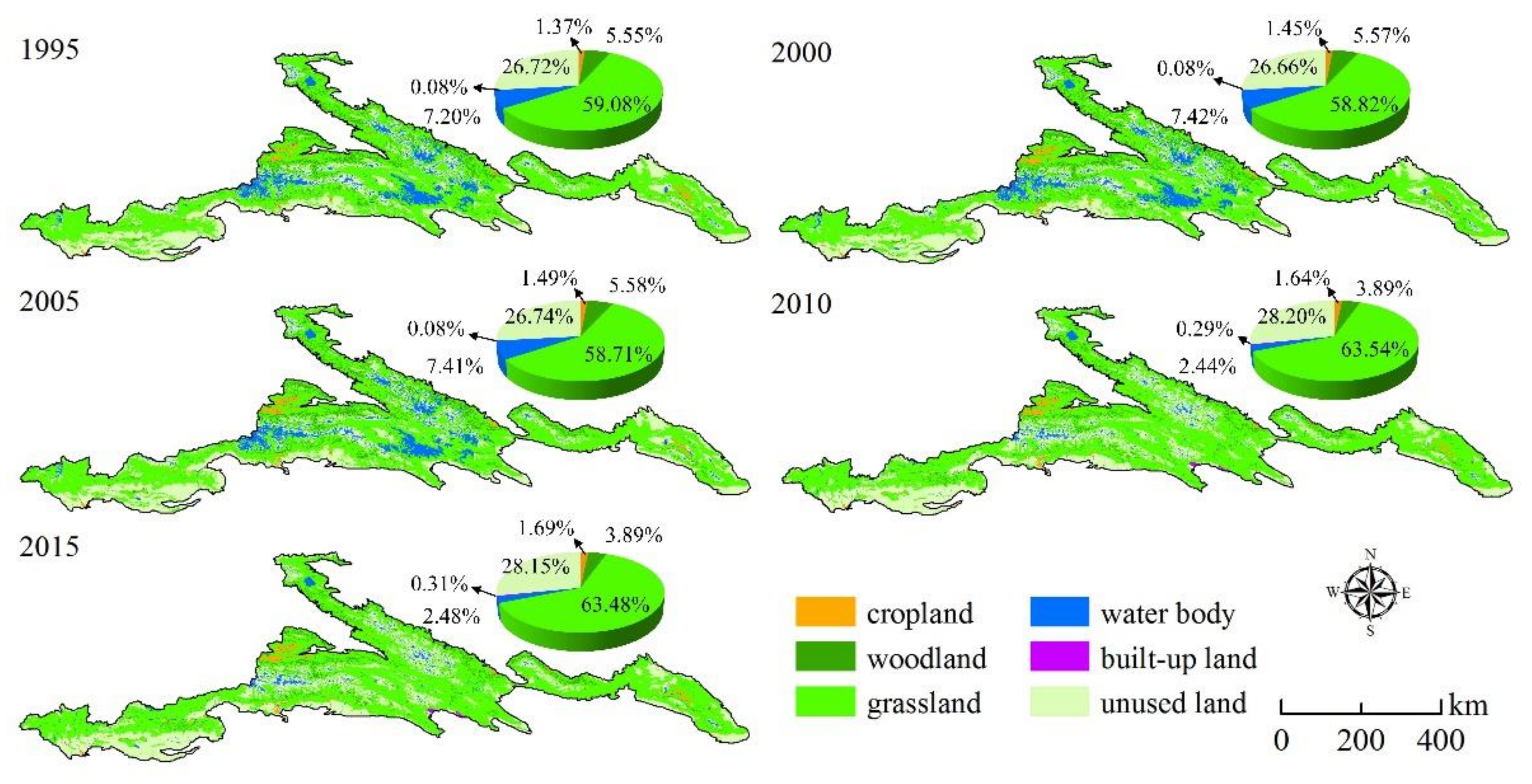
Grassland was the dominant land-use type of the TS, and its total area accounted for almost 60%, followed by unused land (Figure 3). The land-use structure underwent a rapid change during the study period. The areas of cropland, grassland, built-up land, and unused land showed a tendency to increase to varying degrees. The area of grassland and unused land increased the most, reaching 10,345.98 km2 (7.45%) and 3382.57 km2 (5.38%), respectively, and the area of construction land increased the fastest (285.91%). The area of woodland and water body decreased by 3919.17 km2 (30%) and 11,091.12 km2 (65.54%), respectively. Overall, the area of artificial landscape (e.g., cropland and built-up land) increased by 1283.62 km2 (37.55%), while the areas of natural landscape (e.g., woodland, grassland, water body, and unused land) decreased by 1281.74 km2 (0.55%).
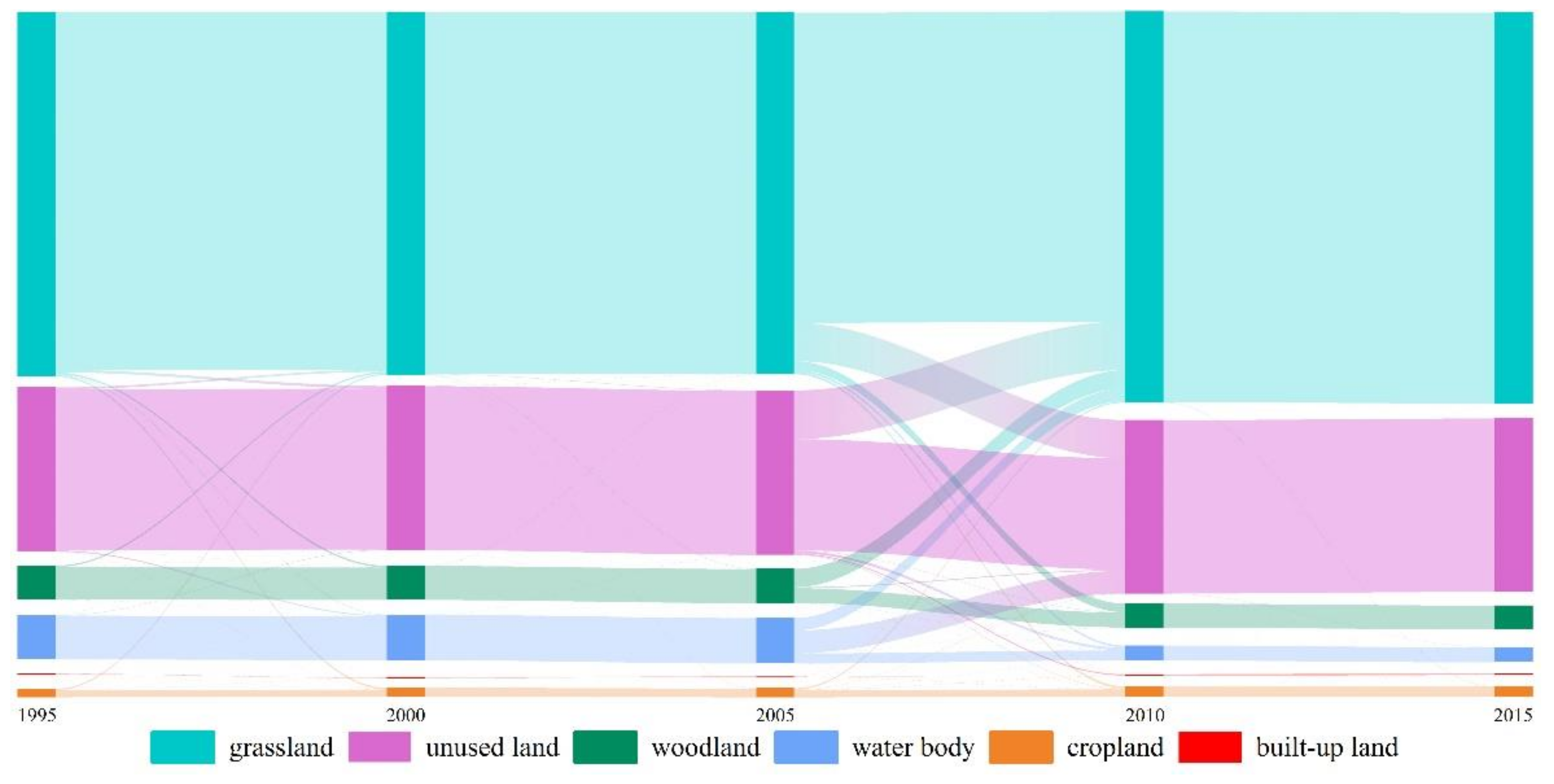
As shown in Figure 4, land-use transitions can be divided into two stages—smooth change (1995–2005) and fast change (2005–2015). From 1995 to 2005, the grassland was mostly transformed into other land-use types, which mainly contained unused land (1085.59 km2), cropland (760.72 km2), and woodland (758.29 km2). The area of unused land transferred out up to 1452.12 km2. From 2005 to 2015, a large amount of unused land was converted to grassland, with an area of 18,563.39 km2. The area of grassland and water body decreased rapidly by 19,711.91 km2 and 13,521.97 km2, respectively. Water bodies were mainly converted into unused land and grassland, while grassland was mainly transformed into unused land and woodland. Overall, under the background of global climate change, ecological land, such as woodlands, grasslands, and water bodies, became more vulnerable. This result is consistent with Wei’s research [16].

3.3. Spatiotemporal Change in Habitat Quality

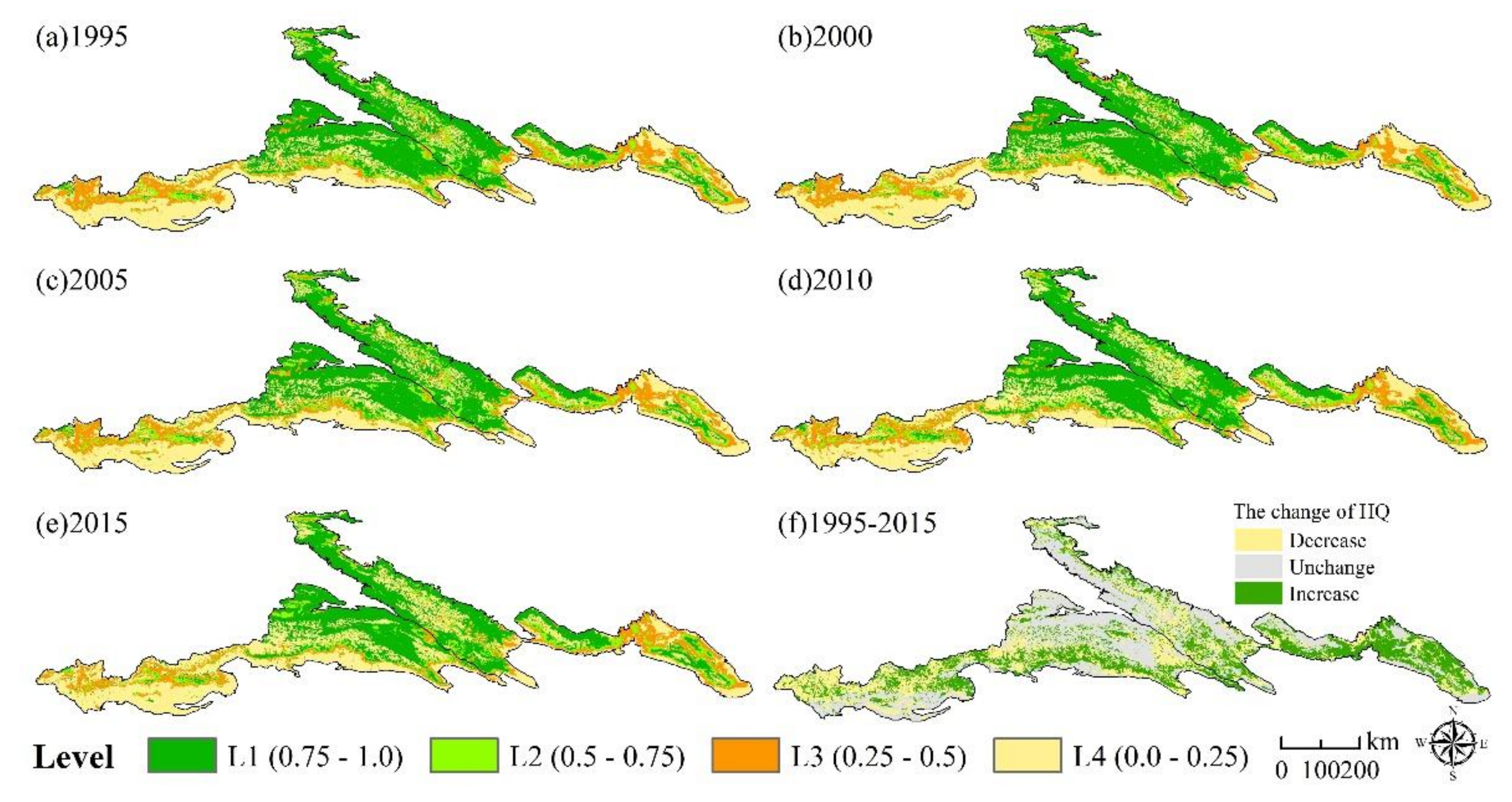
The HQ was divided into four different levels using the equal interval method in ArcGIS 10.5 (Table 5): L1—very important habitat (0.75–1.0); L2—important habitat (0.5–0.75); L3—moderately important habitat (0.25–0.5); and L4—general habitat (0–0.25).
The spatial distribution pattern of HQ in the TS was relatively stable from 1995 to 2015 (Figure 5), with few large areas with significant changes; but, there was still small-scale fluctuation. The NTS had a higher HQ (0.68), followed by the MTS (0.44) and the ETS (0.40). The very important habitat was mainly distributed in the Ili River Valley and the southern edge of the Junggar Basin. These regions were the main distribution areas of forests and grasslands in the TS. The average altitude was above 2700 m and was less disturbed by human activities, which is consistent with previous research [24,43]. The general habitat was mainly distributed in the transitional belt between the southern slope of the middle Tianshan Mountains and the Tarim Basin, which is close to the Taklimakan Desert. There were Gobi desert and bare rock areas with sparse vegetation.
From 1995 to 2015 (Table 5), the average values of the HQ in the TS were 0.5044, 0.5032, 0.5011, 0.4983, and 0.4802, which were at the middle level, with a slight decrease. The HQ of the TS was mainly dominated by very important habitats and general habitats, followed by moderately important habitats and important habitats. In the last 20 years, the areas of L1 and L3 decreased by 1.85 % and 1.88 %, respectively, while the area of L4 increased by 3.69 %, which was mainly due to the substantial glacier shrinkage in the TS caused by rapid warming [15]. The area of L2 was relatively stable.
Altogether, the area with improved HQ reached 30.35% of the study area, mainly in the east. Meanwhile, almost 30.15% of the region faced HQ degradation to different degrees, which was more evident in the western region. The fluctuating change in HQ threatens the biodiversity and ecological security of the Tianshan Mountains.

3.4. The Spatial Heterogeneity of the Habitat Quality

A total of 61,315 grids of 2 × 2 km2 were generated with the “fish net” tool in ArcGIS10.5. From 1995 to 2015, the Global Moran’s I (p < 0.01) values were 0.9024, 0.9034, 0.8989, 0.9028, and 0.9003, respectively, indicating that there was a significant spatial agglomeration of HQ in the TS, but the spatial agglomeration tended to weaken, with a slight decrease in Global Moran’s I.
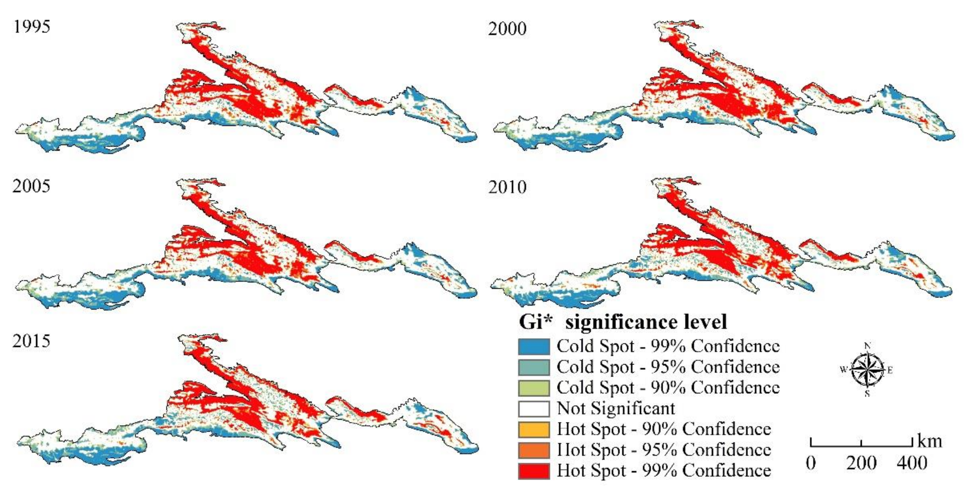
The Getis-Ord G i * was used to identify the spatial heterogeneity in HQ in the TS. There were three non-uniform units (Figure 6): hot spots, cold spots, and random areas. The hot spot areas were mainly distributed in the Ili River Valley and Kaidu River Basin, while the cold spot areas were mainly distributed in the south and east of the Tianshan Mountains. The proportion of hot spot areas in 1995–2015 were 29.62%, 29.75%, 28.79%, 29.6%, and 29.02%, respectively, showing a downward trend. Meanwhile, the proportions of the cold spot areas were 28.40%, 28.90%, 28.17%, 28.63%, and 28.91%, respectively, showing an increasing trend. The proportions of random areas were 41.98%, 41.35%, 43.04%, 41.73%, and 42.07%, respectively. The hot spot areas of PAs in the TS were 17,856 km2, accounting for 25.51% of the total hot spot areas, suggesting that PAs play an important role in maintaining regional biodiversity [24].

3.5. Habitat Quality in Relation to Different PAs

Considering that the boundaries of the World Natural Heritage site were almost the same as those of the nature reserves or nature parks, the HQ of the World Natural Heritage site was not compared, to avoid repeated calculations. Overall, the HQ was strongly affected by the protection level (Figure 7a). Specifically, the nature parks (0.78) had the highest HQ, followed by nature reserves (0.68), the priority areas for biodiversity conservation in the Tianshan Mountains–southwest Junggar Basin (0.65), total Tianshan Mountains (0.50), and unprotected areas (0.47). The average HQ of the PAs was higher than 0.6, whereas that of the unprotected areas was lower than 0.5. Clearly, the establishment of PAs was distinguished in safeguarding important habitats. From 2005 to 2015, the HQ values of the different PA categories fluctuated slightly and were entirely stable. The HQ of the nature parks increased slightly, whereas that of the other PAs showed a downward trend. Among them, the HQ of the nature reserves decreased the most due to the shrinkage of substantial glaciers, up to 0.18, and it was lower than that of the priority areas for biodiversity conservation in the Tianshan Mountains–southwest Junggar Basin.
In terms of the spatial pattern and habitat level (Figure 7b,c), most of the nature reserves and nature parks were distributed in the region of very important habitats and important habitats, both of which covered more than 75% of the area. Nature reserves were mainly distributed in the region of very important habitats, followed by important habitats. Nature parks had an overwhelming superiority of very important habitats, indicating that nature reserves and nature parks play a vital role in supporting ecological security. Nevertheless, conservation effectiveness and design need to be extended beyond the existing PA network to protect an adequate representation of species and habitats [44]. Moreover, we should not only get information on how much area needs protection, but, more importantly, also where to protect biodiversity and habitats.

3.6. Habitat Quality Variation in Terrain Gradient

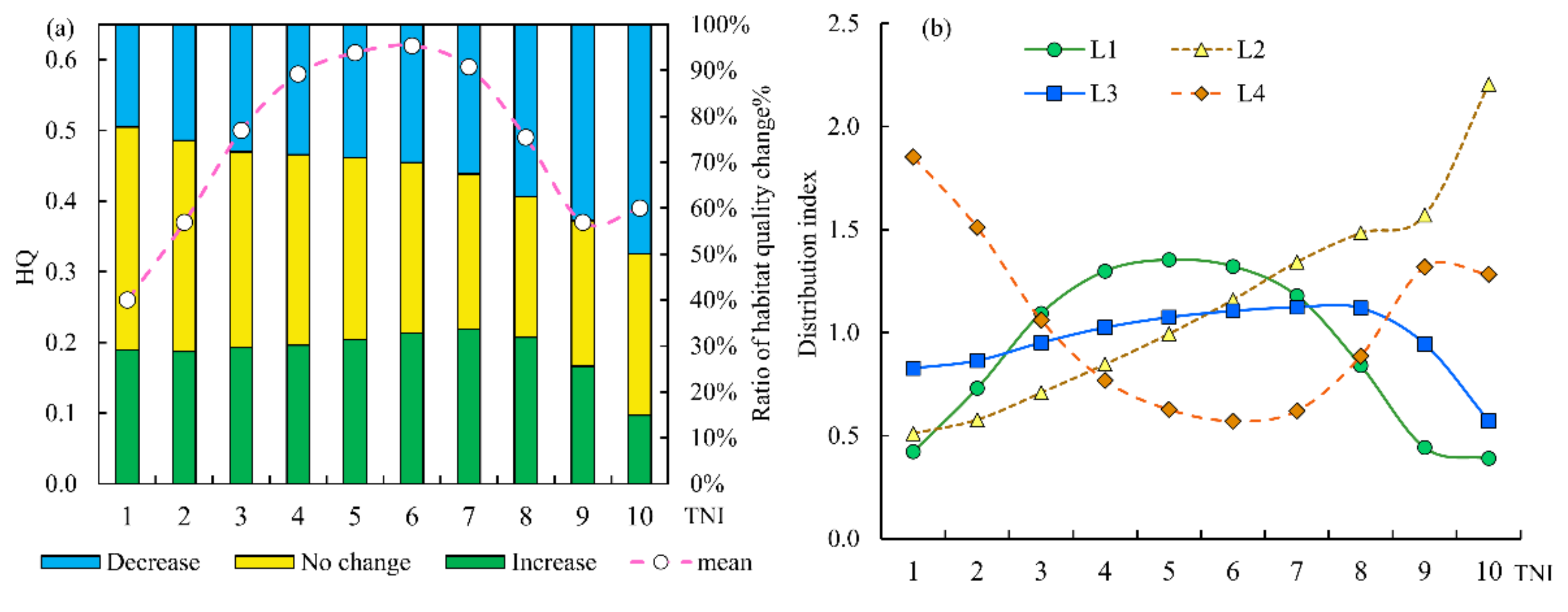
From 1995 to 2015, the HQ at different terrain niches presented three characteristics. First, the HQ showed an inverted “U” type (Figure 8). It increased at TNI 1–5 and decreased at TNI 6–10. The important habitats were mainly distributed at TNI 3–8, which were the main distribution areas of ecological land, such as grassland, forest, and water bodies. Therefore, people should give importance to the monitoring of HQ in these terrain gradient areas. The structure and composition of land use were relatively stable. Second, the HQ impairment and constancy areas increased with the terrain niche index, while the gain areas changed slightly. Third, the distribution index of L1 was greater than 1 at TNI 3–7, which showed a dominant distribution, but habitat quality L4 showed the opposite trend. The distribution index of L2 appeared to be dominant when the TNI was greater than 5. In general, landscape heterogeneity increased at moderate to high terrain levels compared to the low terrain levels in arid mountain ecosystems, indicating that they can support more species, habitat richness, and habitat diversity.

3.7. Driving Factors of Habitat Quality

3.7.1. Comparison of Driving Factors in the Different Sub-Regions

The geographical detector model was utilized to analyze the driving factors (q < 0.01) of HQ in the TS (Figure 9). For the TTS, the driving factors from highest to lowest were SOL, LAND, PRE, TEM, GI, ELE, GDP, RDLS, PD, and TOU. In general, the effect of natural factors on HQ was significantly higher than that of socioeconomic factors. The effects of LAND (−14.93%), PRE (−22.17 %), GDP (−26.36 %), PD (−40.12 %), TOU (−14.76 %), and GI (−31.12 %) all showed a downward trend, while the effects of TEM (11.55 %) and ELE (56.06 %) showed an upward trend, and the effects of SOIL (2.80 %) and RDLS (1.97 %) were relatively stable.
For the ETS, the value of SOL was up to 0.6, and other factors were in the range of 0.2–0.5, besides TOU. The effects of LAND (−10.97 %), PRE (−35.73 %), GDP (−25.66 %), PD (−23.79 %), TOU (−43.93 %), and GI (−27.24 %) all showed a downward trend, while the effects of TEM (11.91 %), ELE (45.48 %), and RDLS (11.91 %) showed an upward trend, and the effect of SOL (3.54 %) showed slight fluctuations.
For the NTS, the first two driving factors were LAND and SOL, and TEM, PRE, ELE, GDP, GI, PD, TOU, and RDLS followed. The effects of LAND (−10.47 %), PRE (−69.01 %), RDLS (−17.32 %), PD (−14.73 %), TOU (−21.19 %), and GI (−35.22 %) all showed a downward trend, and the effects of SOL (12.83 %), TEM (69.01 %), ELE (43.30 %), and GDP (9.16 %) showed an upward trend.
For the MTS, the SOL, LAND, PRE, GI, and TEM were the main influencing factors, followed by ELE, GDP, PD, RDLS, and TOU. The effects of LAND (−18.70 %) and PD (−61.14 %) showed a downward trend, and the effects of TEM (7.60 %), ELE (43.84 %), RDLS (13.87 %), TOU (18.74 %), and GI (11.33 %) showed an upward trend. The effects of SOL (3.94 %), PRE (4.64 %), and GDP (0.95 %) remained almost unchanged.
Our study revealed that both natural factors and anthropogenic activities have varying degrees of effects on HQ, but the influence of natural factors is significantly stronger than human activities. Soil properties, such as soil nutrient status, soil acidification state, and soil moisture, are significant preconditions for vegetation growth. The soil types on the north and south slopes of Tianshan show obvious differences, with the north slope being rich in organic matter and favorable for plant growth, while the south slope is mostly desert and meadow soils, which are not favorable for vegetation growth. Climate factors play a more important role in vegetation sensitivity and resilience in arid and semi-arid regions, and climate variability challenges the stability of vegetation. Abundant precipitation in the Ili Valley and high-altitude mountain areas promotes greening of vegetation, while strong evaporation in the southern Tian Shan, especially in the Taklamakan Desert, inhibits plant growth. Land-use change affects biodiversity by increasing the probability of habitat conversion and fragmentation and lowers the viability of species. Population and economic activities were mainly distributed in piedmont oasis areas because of the high elevation of the TS, and overall, the population density and economic activity intensity were at very low levels. Although the tourist numbers and tourism economy in Xinjiang grew rapidly, the level and scale of tourism development is relatively low compared to those of eastern and central China [45]. Meanwhile, the government planned to cultivate the Tianshan Mountains into a nature-based ecotourism corridor [46]. Grazing is the main use of pastures in the Tian Shan region. Grazing, especially heavy grazing, changes the habitat size and connectivity, threatening the survival of species.

3.7.2. Spatial Interactions between Driving Factors

It is widely accepted that HQ is comprehensively affected by multiple factors; thus, the interaction detector was taken into consideration. The results suggested that the interaction effects on the spatial distribution pattern of HQ were higher than those of single factors for both the total Tianshan Mountains and sub-regions, which showed a double-factor and nonlinear enhancement (Table 6). Overall, the interaction between soil type and land use had the strongest explanatory power because they were the main driving factors. Subsequently, some indistinctive influence factors, such as GDP, PD, and ELE, showed a strong explanatory power in the dynamic interaction processes, demonstrating that HQ was very sensitive to minor changes when the ecosystems were subjected to external disturbances.

4. Discussion

4.1. Climate Change and Anthropogenic Activity Implications

Based on the results, the core driving factors were soil, climate change, land-use change, and grazing. These basic properties (e.g., particle size distribution, clay content, organic matter, and mineral content) in soil support the terrestrial ecosystem and have a great and persistent influence on HQ [47]. Moreover, the impacts of climate change and land-cover change on soil function cannot be ignored [48]. Global biodiversity is affected by climate change and land-use change [3], causing geographic range shifts, expansions and contractions, and decreasing species habitat availability [2,49]. The land-use structure changes, shift in spatial distribution, and increase in intensity of the changes lead to the landscape being dispersed and fragmented, affecting the natural state and integrity of the ecosystem [16]. The interaction effects between climate change and land-use change increased the risk of habitat loss and fragmentation. Thus, appropriate land-use exploitation seems to be a long-term measure to mitigate the impacts of climate change on biodiversity [37]. The leading use of grasslands is in the form of grazing to maintain millions of livelihoods. However, increasing heavy grazing pressure alters plant community composition, diversity, and productivity [18]. Overgrazing is globally regarded as a booster of land degradation and surface erosion [50], which appears to be devastating for biodiversity protection, ecosystem multifunctionality maintenance, and ecosystem services supply, given that rehabilitation is difficult and takes a long time [48]. Hence, grazing pressure management strategies should be strengthened to achieve the goal of grassland ecological restoration.

4.2. The Gap between Conservation Expectations and Reality

A network of PAs is the cornerstone of global biodiversity and plays a key role in preserving rare and endangered species and ecosystems [9]. Consistent with a previous study [24], our results revealed that PAs provide very important habitat protection. There still exist some gaps, as shown in the following: first, the increased fluctuation in habitat quality in the PAs brings challenges to a stable range of species; and second, there is a large spatial mismatch between the distribution of important habitats and PAs.
Poor management is a significant challenge for the PAs in China [51]. As protected species in PAs have specific and strict demands for habitat types and quality, they have limited adaptive capacity to climate change [52]. To enhance the conservation effectiveness of PAs, we suggest the design of a framework for the quantification of the efficiency as the basic requirement and normalization measure [9]. However, it is even more important to strengthen the prediction of climate change impacts on habitats and formulate corresponding strategies to enhance the ability of PAs to adapt to climate change [53].
It has been reported that climate change will expose 84% of mountain species to extinction. Thus, increasing representation in high-elevation reserves is of great value to achieve biodiversity targets after 2020 [49]. It is an urgent and important task to integrate important habitats into the ecological conservation redlines and in the restricted zones in the national ecological function zoning. Forest and grass departments should investigate and identify important habitats and ecosystems and establish an optimized adjustment plan for PAs to repair the ecological gaps in the PA network [51]. Furthermore, integrating protected areas to establish national parks can balance the conflict between ecological conservation and regional development.

4.3. Limitations and Future Work

This study integrated the NDVI and InVEST-HQ module to assess the temporal and spatial variation in HQ over the past 20 years in the Tianshan Mountain ranges. The findings of this study provide further information to expand HQ research on mountain biodiversity and ecosystem services. Despite the merits of our framework, this research still had some limitations that should be addressed in the future. First, owing to the difficulty in obtaining historical threat data, some had to be replaced by adjacent years. In addition, some important threat factors, such as pasture distribution and mining sites, were not calculated in the InVEST-HQ model. Second, with the popular application of remote sensing technology, it could provide a large-scale analysis, long time series, and multiple types of observation data for biodiversity research. The potential and effectiveness of other ecological remote sensing parameters for HQ monitoring and assessment were not compared with NDVI, such as the Enhanced Vegetation Index, Leaf Area Index. Third, future climate change and land-use change scenario simulations and predictions would have been of great value [23,34]. Thus, in the future, it is necessary to make a prediction of HQ to support policy recommendations and guidance for land-use spatial optimization and regional development.

5. Conclusions

Understanding the temporal and spatial variation in HQ and its associated driving factors is the basis for biodiversity conservation and ecosystem management in the context of climate change. This study coupled the NDVI and InVEST-HQ module with higher effectiveness to investigate the HQ change over space and time in the Tianshan Mountains in Xinjiang from 1995 to 2015. The following were found: (1) Natural habitats, such as grassland, was the main body of the research area, and changed the fastest both spatially and quantitatively from 1995 to 2015, as compared to the other habitats. (2) The spatial patterns of the habitats were stable, with the largest areas comprising very important habitats and general habitats, although a slight tendency toward habitat degradation and loss should be highly emphasized. The NTS had a better HQ score than that of the MTS and ETS. (3) The spatial heterogeneity of HQ in the Tianshan Mountains was evident, with the hot spot areas clustered in the Ili River Valley and Kaidu River Basin, and the cold spot areas distributed in the south and east of the Tianshan Mountains. The HQ behaved as an inverted “U” type in the different terrain gradients. Protected areas, such as nature reserves, natural parks, and priority areas for biodiversity conservation, were important for biodiversity protection in the Tianshan ranges, with a HQ score of over 0.5. (4) Natural factors (e.g., soil and climate change) were determined to be the mainstays of HQ, and human factors (e.g., land use and grazing) accelerated the fluctuation in habitat change. Their interaction effects increased conspicuously compared to the those of the single factors. In conclusion, HQ varies due to an elaborate mechanism. Thus, understanding the mechanisms behind the effects of climate change and human activities on mountain HQ will contribute to dynamic governance. These results provide a scientific basis for land-use planning that is adapted to climate change, for the optimal adjustment of PAs, which play a critical role in maintaining mountainous biodiversity and ecosystems.

Author Contributions

Conceptualization, Y.L. and F.H.; methodology, Y.L. and J.Z.; software, J.Z. and Z.W.; validation, Y.L. and Z.Y.; formal analysis, Y.L. and T.R.; investigation, Y.L.; data curation, J.Q.; writing—original draft preparation, Y.L.; writing—review and editing, F.H. and T.R.; visualization, Z.W. and J.Q.; supervision, Z.Y.; project administration, Z.Y.; funding acquisition, F.H. All authors have read and agreed to the published version of the manuscript.

Funding

This research was funded by the Second Tibetan Plateau Scientific Expedition and Research Program (STEP), Grant No. 2019QZKK0401 and the National Natural Science Foundation of China (No. 41971192).

Institutional Review Board Statement

Not applicable.

Informed Consent Statement

Not applicable.

Data Availability Statement

Not applicable.

Conflicts of Interest

The authors declare no conflict of interest.

References

  1. Duraiappah, A.K.; Naeem, S.; Agardy, T.; Ash, N.J.; Cooper, H.D.; Díaz, S.; Faith, D.P.; Mace, G.; McNeely, J.A.; Mooney, H.A.; et al. Ecosystems and Human Well-Being: Biodiversity Synthesis; World Resources Institute: Washington, DC, USA, 2005; p. 86. [Google Scholar]
  2. Powers, R.P.; Jetz, W. Global habitat loss and extinction risk of terrestrial vertebrates under future land-use-change scenarios. Nat. Clim. Chang. 2019, 9, 323–329. [Google Scholar] [CrossRef]
  3. Heikkinen, R.K.; Kartano, L.; Leikola, N.; Aalto, J.; Aapala, K.; Kuusela, S.; Virkkala, R. High-latitude EU Habitats Directive species at risk due to climate change and land use. Glob. Ecol. Conserv. 2021, 28, e01664. [Google Scholar] [CrossRef]
  4. Moreira, M.; Fonseca, C.; Vergílio, M.; Calado, H.; Gil, A. Spatial assessment of habitat conservation status in a Macaronesian island based on the InVEST model: A case study of Pico Island (Azores, Portugal). Land Use Policy 2018, 78, 637–649. [Google Scholar] [CrossRef]
  5. Maes, J.; Paracchini, M.L.; Zulian, G.; Dunbar, M.B.; Alkemade, R. Synergies and trade-offs between ecosystem service supply, biodiversity, and habitat conservation status in Europe. Biol. Conserv. 2012, 155, 1–12. [Google Scholar] [CrossRef]
  6. Payne, D.; Spehn, E.M.; Snethlage, M.; Fischer, M. Opportunities for research on mountain biodiversity under global change. Curr. Opin. Environ. Sustain. 2017, 29, 40–47. [Google Scholar] [CrossRef]
  7. Yu, Y.; Li, J.; Zhou, Z.; Ma, X.; Zhang, X. Response of multiple mountain ecosystem services on environmental gradients: How to respond, and where should be priority conservation? J. Clean. Prod. 2021, 278, 123264. [Google Scholar] [CrossRef]
  8. Kohler, T.; Maselli, D. (Eds.) Mountains and Climate Change. From Understanding to Action, 3rd ed.; Geographica Bernensia: Bern, Switzerland, 2012. [Google Scholar]
  9. Vincent, C.; Fernandes, R.F.; Cardoso, A.R.; Broennimann, O.; Di Cola, V.; D’Amen, M.; Ursenbacher, S.; Schmidt, B.R.; Pradervand, J.-N.; Pellissier, L.; et al. Climate and land-use changes reshuffle politically-weighted priority areas of mountain biodiversity. Glob. Ecol. Conserv. 2019, 17, e00589. [Google Scholar] [CrossRef]
  10. Grêt-Regamey, A.; Weibel, B. Global assessment of mountain ecosystem services using earth observation data. Ecosyst. Serv. 2020, 46, 101213. [Google Scholar] [CrossRef]
  11. Bernardino, P.N.; De Keersmaecker, W.; Fensholt, R.; Verbesselt, J.; Somers, B.; Horion, S.; Silva, T. Global-scale characterization of turning points in arid and semi-arid ecosystem functioning. Glob. Ecol. Biogeogr. 2020, 29, 1230–1245. [Google Scholar] [CrossRef] [Green Version]
  12. McNeely, J.A. Biodiversity in arid regions: Values and perceptions. J. Arid. Environ. 2003, 54, 61–70. [Google Scholar] [CrossRef]
  13. Zhang, H.X.; Zhang, M.L. Spatial Patterns of Species Diversity and Phylogenetic Structure of Plant Communities in the Tianshan Mountains, Arid Central Asia. Front. Plant Sci. 2017, 8, 2134. [Google Scholar] [CrossRef] [PubMed] [Green Version]
  14. Fan, M.; Xu, J.; Chen, Y.; Li, W. Reconstructing high-resolution temperature for the past 40 years in the Tianshan Mountains, China based on the Earth system data products. Atmos. Res. 2021, 253, 105493. [Google Scholar] [CrossRef]
  15. Chen, Y.; Li, W.; Deng, H.; Fang, G.; Li, Z. Changes in Central Asia’s Water Tower: Past, Present and Future. Sci. Rep. 2016, 6, 35458. [Google Scholar] [CrossRef]
  16. Wei, H.; Xiong, L.; Tang, G.; Strobl, J.; Xue, K. Spatial–temporal variation of land use and land cover change in the glacial affected area of the Tianshan Mountains. Catena 2021, 202, 105256. [Google Scholar] [CrossRef]
  17. Li, Y.; Chen, Y.; Sun, F.; Li, Z. Recent vegetation browning and its drivers on Tianshan Mountain, Central Asia. Ecol. Indic. 2021, 129, 107912. [Google Scholar] [CrossRef]
  18. Zhao, W.Y.; Li, J.L.; Qi, J.G. Changes in vegetation diversity and structure in response to heavy grazing pressure in the northern Tianshan Mountains, China. J. Arid. Environ. 2007, 68, 465–479. [Google Scholar] [CrossRef]
  19. Sharp, R.; Tallis, H.T.; Ricketts, T.; Guerry, A.D.; Wood, S.A.; Chaplin-Kramer, R.; Nelson, E.; Ennaanay, D.; Wolny, S.; Olwero, N.; et al. InVEST+ VERSION+ User’s Guide; The Natural Capital Project; Stanford University: Stanford, CA, USA; University of Minnesota: Minneapolis, MN, USA; The Nature Conservancy, and World Wildlife Fund: Arlington, VT, USA, 2015. [Google Scholar]
  20. Riedler, B.; Lang, S. A spatially explicit patch model of habitat quality, integrating spatio-structural indicators. Ecol. Indic. 2018, 94, 128–141. [Google Scholar] [CrossRef]
  21. Sun, X.; Jiang, Z.; Liu, F.; Zhang, D. Monitoring spatio-temporal dynamics of habitat quality in Nansihu Lake basin, eastern China, from 1980 to 2015. Ecol. Indic. 2019, 102, 716–723. [Google Scholar] [CrossRef]
  22. Zhu, C.; Zhang, X.; Zhou, M.; He, S.; Gan, M.; Yang, L.; Wang, K. Impacts of urbanization and landscape pattern on habitat quality using OLS and GWR models in Hangzhou, China. Ecol. Indic. 2020, 117, 106654. [Google Scholar] [CrossRef]
  23. He, J.; Huang, J.; Li, C. The evaluation for the impact of land use change on habitat quality: A joint contribution of cellular automata scenario simulation and habitat quality assessment model. Ecol. Model. 2017, 366, 58–67. [Google Scholar] [CrossRef]
  24. Sallustio, L.; De Toni, A.; Strollo, A.; Di Febbraro, M.; Gissi, E.; Casella, L.; Geneletti, D.; Munafò, M.; Vizzarri, M.; Marchetti, M. Assessing habitat quality in relation to the spatial distribution of protected areas in Italy. J. Environ. Manag. 2017, 201, 129–137. [Google Scholar] [CrossRef] [PubMed]
  25. Di Febbraro, M.; Sallustio, L.; Vizzarri, M.; De Rosa, D.; De Lisio, L.; Loy, A.; Eichelberger, B.A.; Marchetti, M. Expert-based and correlative models to map habitat quality: Which gives better support to conservation planning? Glob. Ecol. Conserv. 2018, 16, e00513. [Google Scholar] [CrossRef]
  26. Nagendra, H.; Lucas, R.; Honrado, J.P.; Jongman, R.H.G.; Tarantino, C.; Adamo, M.; Mairota, P. Remote sensing for conservation monitoring: Assessing protected areas, habitat extent, habitat condition, species diversity, and threats. Ecol. Indic. 2013, 33, 45–59. [Google Scholar] [CrossRef]
  27. Pettorelli, N.; Ryan, S.; Mueller, T.; Bunnefeld, N.; Jedrzejewska, B.; Lima, M.; Kausrud, K. The Normalized Difference Vegetation Index (NDVI): Unforeseen successes in animal ecology. Clim. Res. 2011, 46, 15–27. [Google Scholar] [CrossRef]
  28. Aizen, V.; Aizen, E.; Melack, J.; Dozier, J. Climatic and Hydrologic Changes in the Tien Shan, Central Asia. J. Clim. 1997, 10, 1393–1404. [Google Scholar] [CrossRef]
  29. Mittermeier, R.A.; Turner, W.R.; Larsen, F.W.; Brooks, T.M.; Gascon, C. Global Biodiversity Conservation: The Critical Role of Hotspots. In Biodiversity Hotspots; Springer: Berlin/Heidelberg, Germany, 2011; pp. 3–22. [Google Scholar] [CrossRef]
  30. Olson, D.M.; Dinerstein, E. The Global 200: Priority ecoregions for global conservation. Ann. Mo. Bot. Gard. 2002, 89, 199–224. [Google Scholar] [CrossRef]
  31. Ministry of Ecology and Environment of People’s Republic of China. China National Biodiversity Conservation Strategy and Action Plan (2011–2030); China Environmental Science Press: Beijing, China, 2010.
  32. Shui, Y.; Lu, H.; Wang, H.; Yan, Y.; Wu, G. Assessment of habitat quality on the basis of land cover and NDVI changes in Lhasa River Basin (in Chinese). Acta Ecol. Sin. 2018, 38, 8949–8954. [Google Scholar] [CrossRef]
  33. Zhao, X.; Wang, J.; Su, J.; Sun, W.; Jin, W. Assessment of habitat quality and degradation degree based on InVEST model and Moran index in Gansu Province, China. Trans. Chin. Soc. Agric. Eng. 2020, 36, 301–308. (In Chinese) [Google Scholar] [CrossRef]
  34. Liu, F.T.; Xu, E.Q. Comparison of spatial-temporal evolution of habitat quality between Xinjiang Corps and Non-corps Region based on land use. Chin. J. Appl. Ecol. 2020, 31, 2341–2351. (In Chinese) [Google Scholar] [CrossRef]
  35. Xue, L.; Zhu, B.; Wu, Y.; Wei, G.; Liao, S.; Yang, C.; Wang, J.; Zhang, H.; Ren, L.; Han, Q. Dynamic projection of ecological risk in the Manas River basin based on terrain gradients. Sci. Total Environ. 2019, 653, 283–293. [Google Scholar] [CrossRef]
  36. McBratney, A.; Field, D.J.; Koch, A. The dimensions of soil security. Geoderma 2014, 213, 203–213. [Google Scholar] [CrossRef] [Green Version]
  37. Hülber, K.; Kuttner, M.; Moser, D.; Rabitsch, W.; Schindler, S.; Wessely, J.; Gattringer, A.; Essl, F.; Dullinger, S. Habitat availability disproportionally amplifies climate change risks for lowland compared to alpine species. Glob. Ecol. Conserv. 2020, 23, e01113. [Google Scholar] [CrossRef]
  38. Liu, C.; Wang, C.; Liu, L. Spatio-temporal variation on habitat quality and its mechanism within the transitional area of the Three Natural Zones: A case study in Yuzhong county. Geogr. Res. 2018, 37, 419–432. (In Chinese) [Google Scholar] [CrossRef]
  39. Fang, L.; Wang, L.; Chen, W.; Sun, J.; Cao, Q.; Wang, S.; Wang, L. Identifying the impacts of natural and human factors on ecosystem service in the Yangtze and Yellow River Basins. J. Clean. Prod. 2021, 314, 127995. [Google Scholar] [CrossRef]
  40. Wang, J.-F.; Zhang, T.-L.; Fu, B.-J. A measure of spatial stratified heterogeneity. Ecol. Indic. 2016, 67, 250–256. [Google Scholar] [CrossRef]
  41. Song, Y.; Wang, J.; Ge, Y.; Xu, C. An optimal parameters-based geographical detector model enhances geographic characteristics of explanatory variables for spatial heterogeneity analysis: Cases with different types of spatial data. GISci. Remote Sens. 2020, 57, 593–610. [Google Scholar] [CrossRef]
  42. Zhang, H.; Qian, Y.; Wu, Z.; Wang, Z. Vegetation-environment relationships between northern slope of Karlik Mountain and Naomaohu Basin, East Tianshan Mountains. Chin. Geogr. Sci. 2012, 22, 288–301. [Google Scholar] [CrossRef]
  43. Yang, Y. Evolution of habitat quality and association with land-use changes in mountainous areas: A case study of the Taihang Mountains in Hebei Province, China. Ecol. Indic. 2021, 129, 107967. [Google Scholar] [CrossRef]
  44. De Alban, J.D.T.; Leong, B.P.I.; Venegas-Li, R.; Connette, G.M.; Jamaludin, J.; Latt, K.T.; Oswald, P.; Reeder, C.; Webb, E.L. Conservation beyond the existing protected area network is required to improve species and habitat representation in a global biodiversity hotspot. Biol. Conserv. 2021, 257, 109105. [Google Scholar] [CrossRef]
  45. Wang, T.; Wu, P.; Ge, Q.; Ning, Z. Ticket prices and revenue levels of tourist attractions in China: Spatial differentiation between prefectural units. Tour. Manag. 2021, 83, 104214. [Google Scholar] [CrossRef]
  46. Xinjiang Uygur Autonomous Region Development and Reform Commission; Xinjiang Uygur Autonomous Region Tourism Development Commission. Xinjiang Uygur Autonomous Region Thirteenth Five-Year Plan for Tourism Development; Xinjiang Uygur Autonomous Region Development and Reform Commission; Xinjiang Uygur Autonomous Region Tourism Development Commission: Urumqi, China, 2017. [Google Scholar]
  47. Jost, E.; Schonhart, M.; Skalsky, R.; Balkovic, J.; Schmid, E.; Mitter, H. Dynamic soil functions assessment employing land use and climate scenarios at regional scale. J. Environ. Manag. 2021, 287, 112318. [Google Scholar] [CrossRef] [PubMed]
  48. Albaladejo, J.; Díaz-Pereira, E.; de Vente, J. Eco-Holistic Soil Conservation to support Land Degradation Neutrality and the Sustainable Development Goals. Catena 2021, 196, 104823. [Google Scholar] [CrossRef]
  49. Manes, S.; Costello, M.J.; Beckett, H.; Debnath, A.; Devenish-Nelson, E.; Grey, K.-A.; Jenkins, R.; Khan, T.M.; Kiessling, W.; Krause, C.; et al. Endemism increases species’ climate change risk in areas of global biodiversity importance. Biol. Conserv. 2021, 257, 109070. [Google Scholar] [CrossRef]
  50. Donovan, M.; Monaghan, R. Impacts of grazing on ground cover, soil physical properties and soil loss via surface erosion: A novel geospatial modelling approach. J. Environ. Manag. 2021, 287, 112206. [Google Scholar] [CrossRef]
  51. Zhang, L.; Luo, Z.; Mallon, D.; Li, C.; Jiang, Z. Biodiversity conservation status in China’s growing protected areas. Biol. Conserv. 2017, 210, 89–100. [Google Scholar] [CrossRef]
  52. Li, X.; Clinton, N.; Si, Y.; Liao, J.; Liang, L.; Gong, P. Projected impacts of climate change on protected birds and nature reserves in China. Sci. Bull. 2015, 60, 1644–1653. [Google Scholar] [CrossRef] [Green Version]
  53. Tanner-McAllister, S.L.; Rhodes, J.; Hockings, M. Managing for climate change on protected areas: An adaptive management decision making framework. J. Environ. Manag. 2017, 204, 510–518. [Google Scholar] [CrossRef]
Figure 1. Location of study area (Map number: Xin S (2021) 023).
Land 11 01805 g001
Figure 2. The validation of habitat quality based on species richness.
Land 11 01805 g002
Figure 3. The land-use change from 1995 to 2015.
Land 11 01805 g003
Figure 4. Land-use transitions from 1995 to 2015.
Land 11 01805 g004
Figure 5. The change in habitat quality from 1995 to 2015. Notes: (a)~(e) are the spatial distribution of different habitat quality levels in 1995, 2000, 2005, 2010, and 2015, respectively; (f) is the change of habitat quality from 1995 to 2015.
Land 11 01805 g005
Figure 6. Getis-Ord G i * scores of habitat quality.
Land 11 01805 g006
Figure 7. The change in habitat quality of the different PA categories (a), the average habitat quality from 1995 to 2015 (b), and the proportion of each different habitat quality level of the nature reserves and nature parks (c). Notes: I is nature reserve, II is nature park, III is the priority areas for biodiversity conservation in the Tianshan Mountains–southwest Junggar Basin, IV is total Tianshan Mountains, and V is unprotected areas.
Land 11 01805 g007
Figure 8. The habitat quality change from 1995 to 2015 (a), and the distribution index of habitat quality level at different terrain niches (b).
Land 11 01805 g008
Figure 9. The PD value of each factor from 1995 to 2015: (a) the total Tianshan Mountains area, (b) the east Tianshan Mountains, (c) the north Tianshan Mountains, and (d) the middle Tianshan Mountains.
Land 11 01805 g009
Table 1. Maximum influence distance and weight of the threat factors in TS.
ThreatsMaximum Influence Distance/kmWeightSpatial Decay Type
Cropland80.7linear
Urban land101linear
Rural residential60.6linear
Other construction land80.8linear
Railway40.5linear
Highway30.4linear
Table 2. Sensitivity of different habitat types to different threat factors.
Land-Use CodeHabitatCroplandUrban LandRural
Residential
Other
Construction Land
RailwayHighway
100.30.00.60.40.30.50.4
2110.80.90.80.80.80.7
220.90.60.70.60.50.60.5
230.80.70.80.70.60.80.7
240.70.70.80.70.60.70.6
310.90.50.60.50.40.50.6
320.80.60.70.60.40.50.6
330.70.70.80.70.60.50.6
4110.10.70.60.50.50.4
4210.10.70.60.50.50.4
4310.10.70.60.50.50.4
4410.10.10.20.10.50.4
450.80.70.80.60.50.50.4
510000000
520000000
530000000
610000000
620000000
630.10.10.10.10.10.20.2
640.80.10.50.60.40.50.7
650.10.10.10.10.10.20.2
660000000
670000000
Notes: 10 is cropland, 21 is forestland, 22 is shrub wood, 23 is sparse woods, 24 is other woodland, 31 is high coverage grassland, 32 is moderate coverage grassland, 33 is low coverage grassland, 41 is river and canal, 42 is lake, 43 is reservoir and pond, 44 is permanent glaciers, 45 is mudflats, 51 is urban land, 52 is rural settlements, 53 is other construction land, 61 is sand land, 62 is Gobi, 63 is saline-alkali lands, 64 is wetland, 65 is bare land, 66 is bare rock texture, and 67 is other unused land.
Table 3. Details of the driving factors.
IndexCodeUnitData Source and Calculation
Soil typeSOL-Data from RESDC
Annual mean precipitationPREmmData from RESDC
Annual mean temperatureTEM°CData from RESDC
ElevationELEmData from the Geospatial Data Cloud (http://www.gscloud.cn, accessed on 21 April 2022)
Relief degree of land surfaceRDLS-Extract from DEM
Land-use typeLAND-Data from RESDC
Gross domestic productGPD104CNY/km2Data from RESDC
Population densityPDperson/km2Data from RESDC
Distance to tourism attractionsTOUmThe tourism attractions were obtained from the Department of Culture and Tourism of the Xinjiang Uygur Autonomous Region. It was calculated by ArcGIS “Euclidean distance” tool.
Grazing intensityGIheads/km2The livestock data was obtained from the XinJiang Statistical Yearbook. The grazing intensity was calculated based on literature (Li et al., 2014).
Table 4. Types of interaction between driving factors (Xs).
DescriptionInteraction
q(X1∩X2) < Min(q(X1), q(X2))Weaken, nonlinear
Min(q(X1), q(X2)) < q(X1∩X2) < Max(q(X1), q(X2))Weaken, univariate, nonlinear
q(X1∩X2) > Max(q(X1), q(X2))Enhance, linear, bivariate
q(X1∩X2) = q(X1) + q(X2)Independent
q(X1∩X2) > q(X1) + q(X2)Enhance, nonlinear
Table 5. The area of different habitat quality levels.
ClassificationLevelValueArea (%)
19952000200520102015
Very important habitatL10.75~1.037.0837.7636.1537.0535.23
Important habitatL20.5~0.7510.659.6011.7810.8710.69
Moderately important habitatL30.25~0.516.8615.7616.4715.2914.98
General habitatL40.0~0.2535.4136.8835.6136.7839.10
Table 6. The dominant interactions between two driving factors in different zones.
YearZoneMain Interaction Detector
1995TTSSOL∩LAND, GI∩LAND, GI∩SOL
ETSSOL∩LAND, GDP∩SOL, PRE∩LAND
NTSSOL∩LAND, PRE∩LAND, GI∩LAND
MTSSOL∩LAND, GI∩SOL, ELE∩SOL
2000TTSSOL∩LAND, PRE∩LAND, GI∩SOL
ETSSOL∩LAND, GDP∩SOL, PD∩SOL
NTSSOL∩LAND, PRE∩LAND, GI∩LAND
MTSGI∩SOL, SOL∩LAND, ELE∩PRE
2005TTSSOL∩LAND, GI∩SOL, GDP∩SOL
ETSGDP∩SOL, SOL∩LAND, PD∩SOL
NTSSOL∩LAND, ELE∩LAND, GI∩LAND
MTSSOL∩LAND, GI∩SOL, ELE∩SOL
2010TTSSOL∩LAND, ELE∩SOL, GDP∩SOL
ETSSOL∩LAND, GDP∩SOL, PD∩SOL
NTSSOL∩LAND, PRE∩LAND, GI∩LAND
MTSELE∩SOL, GI∩SOL, GDP∩SOL
2015TTSSOL∩LAND, ELE∩SOL, GDP∩SOL
ETSSOL∩LAND, ELE∩SOL, PD∩SOL
NTSSOL∩LAND, ELE∩LAND, TEM∩LAND
MTSELE∩SOL, GI∩SOL, ELE∩PRE
Publisher’s Note: MDPI stays neutral with regard to jurisdictional claims in published maps and institutional affiliations.