
A New Indicator to Better Represent the Impact of Landscape Pattern Change on Basin Soil Erosion and Sediment Yield in the Upper Reach of Ganjiang, China

 ,
,  and
and
Abstract
:1. Introduction
2. Materials and Methods
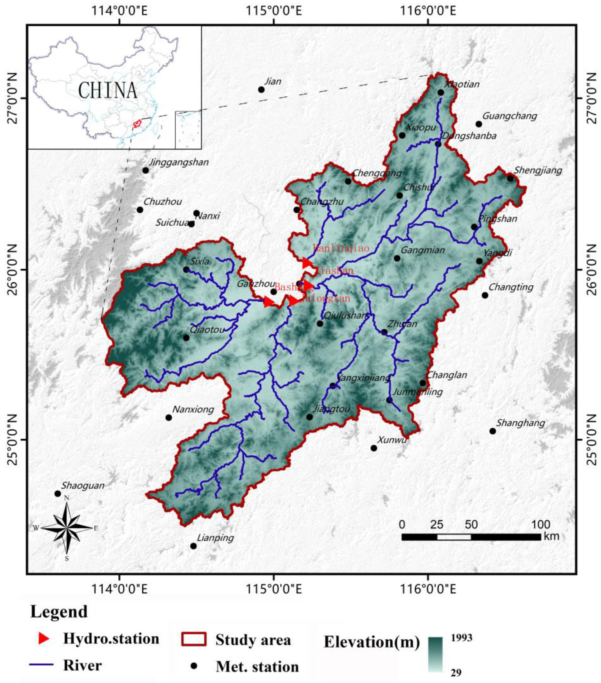
2.1. Study Area
2.2. SWAT Model Simulations
2.3. Partial Least-Squares Regression
2.4. Design of Combinations
- Combination 1:
- land use in each year.
- Combination 2:
- land use in each year + LS + K.
- Combination 3:
- combination 2 + C.
- Combination 4:
- combination 2 + R.
- Combination 5:
- combination 2 + C + R.
3. Results
3.1. Model Calibration and Validation
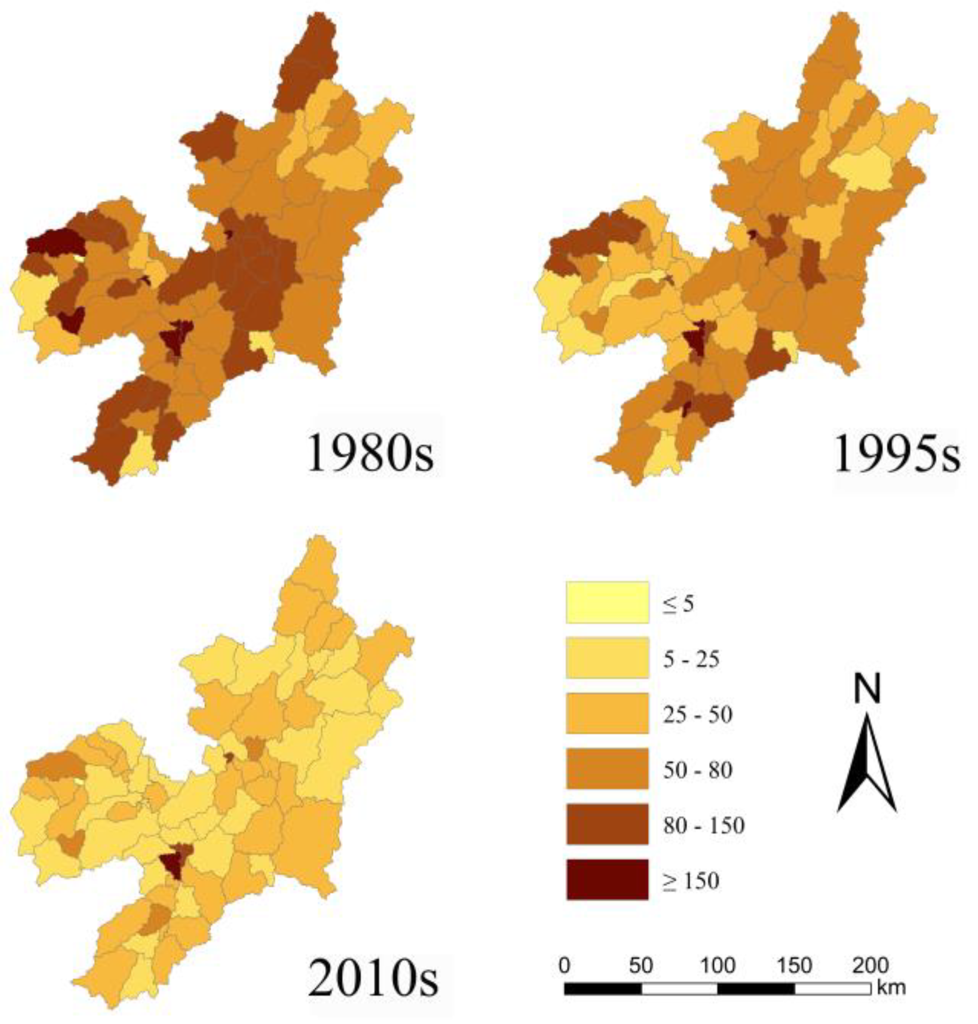
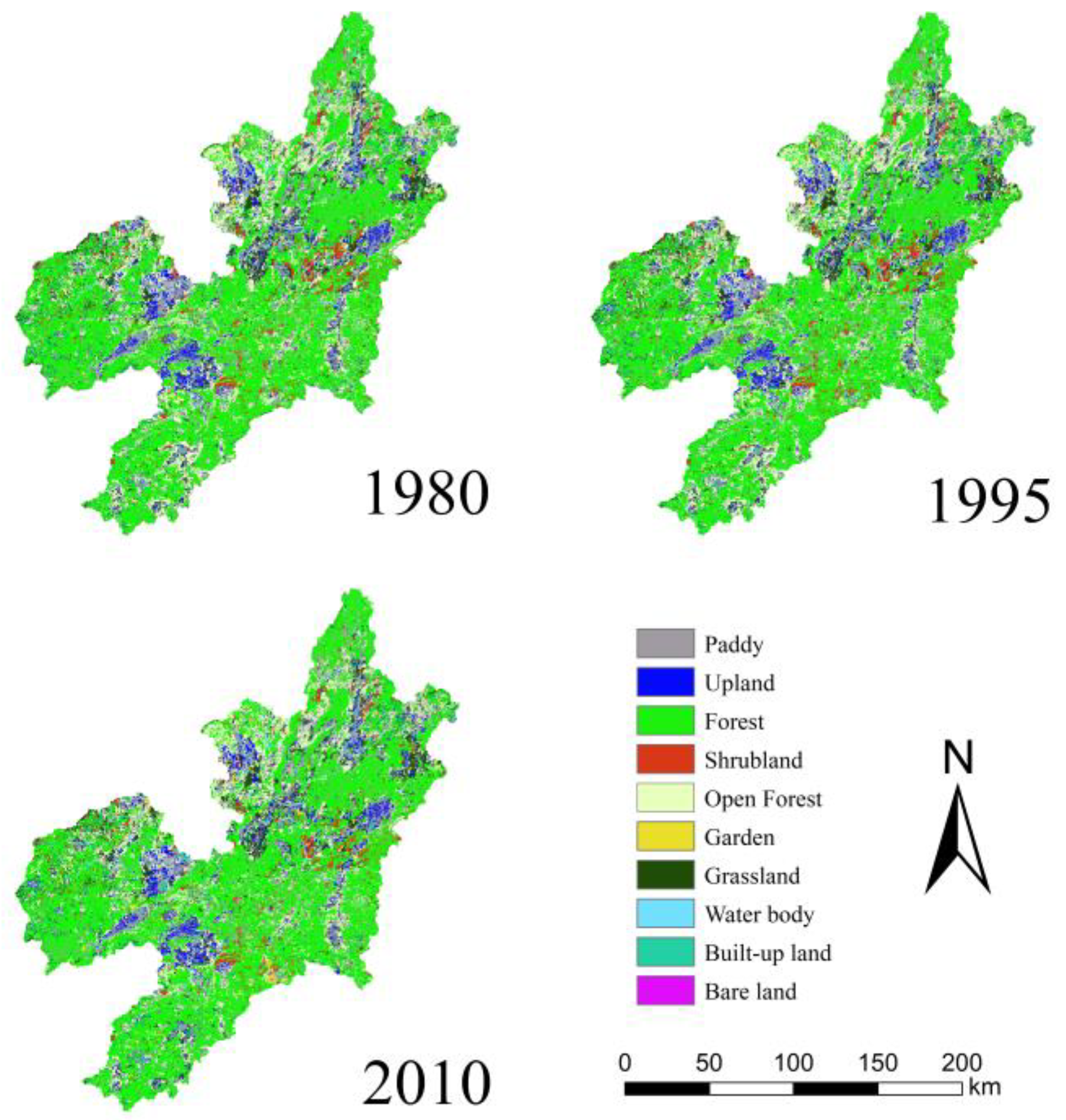
3.2. Analysis of Land Use, Soil Erosion, and Sediment Yield Changes
3.3. Correlation Analysis of Landscape Metrics in Different Combinations
3.4. Correlation Analysis of the Soil Erosion and Landscape Metrics in Different Combinations
3.5. Correlation Analysis of Sediment Yield and the Landscape Metrics in Different Combinations
3.6. Quantification of the Correlations between Soil Erosion or Sediment Yield and Landscape Metrics
4. Discussion
5. Conclusions
- (1)
- In the 1980s–2010s, the areas of other wooded lands and construction lands in the upper Ganjiang Basin increased to large degrees, which was related to economic factors such as urban expansion, afforestation, and extensive development of economic forests. This period also saw considerable decreases in the soil erosion and sediment yield of the river basin, reflecting the great importance attached by the local authorities to water and soil conservation efforts that effectively restored the ecological environment.
- (2)
- Five combinations were established through the addition of the relatively fixed soil erosion factors (i.e., the LS and K factors) and/or one or both of the dynamically varying C and R factors to the land-use. The correlations between the landscape metrics in each combination were calculated. When we compared the correlations between the landscape metrics across the five combinations, highly similar correlations were found between the area metrics, between the fragmentation metrics, between the spatial structure metrics, and between the evenness metrics in the different combinations. However, the correlations between the shape metrics in Combination 1 differed considerably from those in the other combinations.
- (3)
- Comparison of the correlations between the landscape metrics in different combinations and the soil erosion and sediment yield of the river basin showed that the landscape metrics in Combination 4, which combined the land-use and the LS, K, and R factors, were the most significantly correlated with soil erosion and sediment yield. The correlations between the landscape metrics with the highest VIP scores in Combination 4 and the soil erosion and sediment yield in the river basin were quantified. This study explores a new indicator for the correlations between landscape metrics and soil erosion and sediment yield and provides decision-makers with a new quantification method for evaluating these correlations and formulating water and soil conservation policies. While we attempted to explain why the landscape indicator in Combination 4 were the most significantly correlated with the soil erosion and sediment yield in the river basin, further research is needed to determine the relevant internal principles and mechanisms of action from a landscape pattern perspective.
Author Contributions
Funding
Institutional Review Board Statement
Informed Consent Statement
Data Availability Statement
Conflicts of Interest
References
- Forman, R.T.T. Land Mosaics: The Ecology of Landscapes and Regions; Cambridge University Press: Cambridge, UK, 1995. [Google Scholar]
- Turner, M.G. Landscape Ecology: The Effect of Pattern on Process. Annu. Rev. Ecol. Syst. 1989, 20, 171–197. [Google Scholar] [CrossRef]
- Ludwig, J.A.; Bastin, G.N.; Chewings, V.H.; Eager, R.W.; Liedloff, A.C. Leakiness: A new index for monitoring the health of arid and semiarid landscapes using remotely sensed vegetation cover and elevation data. Ecol. Indic. 2007, 7, 442–454. [Google Scholar] [CrossRef]
- Huang, Z.; Tian, Y.; Xiao, W.; Ma, D. Effects of landscape patterns on runoff and sediment export from typical agroforestry watersheds in the Three Gorges Reservoir area, China. Acta Ecol. Sin. 2013, 33, 7487–7495. [Google Scholar] [CrossRef]
- Wei, O.; Skidmore, A.K.; Hao, F.; Wang, T. Soil erosion dynamics response to landscape pattern. Sci. Total Environ. 2010, 408, 1358–1366. [Google Scholar]
- Fu, B.-J.; Wang, Y.; Lu, Y.; He, C.; Chen, L.-D.; Song, C.-J. The effects of land-use combinations on soil erosion: A case study in the Loess Plateau of China. Prog. Phys. Geogr. 2009, 33, 793–804. [Google Scholar] [CrossRef]
- Liu, Y.; Lü, Y.; Fu, B.-J. Implication and limitation of landscape metrics in delineating relationship between landscape pattern and soil erosion. Acta Ecol. Sin. 2011, 31, 267–275. [Google Scholar]
- Hulshoff, R.M. Landscape indices describing a Dutch landscape. Landsc. Ecol. 1995, 10, 101–111. [Google Scholar] [CrossRef]
- Shi, Z.H.; Ai, L.; Li, X.; Huang, X.D.; Wu, G.L.; Liao, W. Partial least-squares regression for linking land-cover patterns to soil erosion and sediment yield in watersheds. J. Hydrol. 2013, 498, 165–176. [Google Scholar] [CrossRef]
- Dash, C.B.; Fraterrigo, J.M.; Hu, F.S. Land cover influences boreal-forest fire responses to climate change: Geospatial analysis of historical records from Alaska. Landsc. Ecol. 2016, 31, 1781–1793. [Google Scholar] [CrossRef]
- Venne, L.S.; Tsai, J.S.; Cox, S.B.; Smith, L.M.; Mcmurry, S.T. Amphibian Community Richness in Cropland and Grassland Playas in the Southern High Plains, USA. Wetlands 2012, 32, 619–629. [Google Scholar] [CrossRef]
- Zheng, C.; Zhi, F.X.; Lei, W. Landscape Structure Analysis of Xiao’shao Reclaimed Area Based on Remote Sensing Image. Remote Sens. Inf. 2003, 4, 28–32. [Google Scholar]
- Shehab, Z.N.; Jamil, N.R.; Aris, A.Z.; Shafie, N.S. Spatial variation impact of landscape patterns and land use on water quality across an urbanized watershed in Bentong, Malaysia. Ecol. Indic. 2021, 122, 107254. [Google Scholar] [CrossRef]
- Boongaling, C.G.K.; Faustino-Eslava, D.V.; Lansigan, F.P. Modeling land use change impacts on hydrology and the use of landscape metrics as tools for watershed management: The case of an ungauged catchment in the Philippines. Land Use Policy 2018, 72, 116–128. [Google Scholar] [CrossRef]
- Wang, J.; Yang, L.; Wei, W.; Chen, L.; Huang, Z. Effects of landscape pattern on watershed soil erosion and sediment delivery in hilly and gully region of the Loess Plateau of China: Patch class-level. Acta Ecol. Sin. 2011, 31, 5739–5748. [Google Scholar]
- Corry, R.C.; Nassauer, J.I. Limitations of using landscape pattern indices to evaluate the ecological consequences of alternative plans and designs. Landsc. Urban Plan. 2005, 72, 265–280. [Google Scholar] [CrossRef]
- Yan, B.; Fang, N.F.; Zhang, P.C.; Shi, Z.H. Impacts of land use change on watershed streamflow and sediment yield: An assessment using hydrologic modelling and partial least squares regression. J. Hydrol. 2013, 484, 26–37. [Google Scholar] [CrossRef]
- Carrascal, L.M.; Galván, I.; Gordo, O. Partial least squares regression as an alternative to current regression methods used in ecology. Oikos 2009, 118, 681–690. [Google Scholar] [CrossRef]
- Renard, K.; Foster, G.; Weesies, G.; McCool, D.; Yoder, D. Predicting soil erosion by water: A guide to conservation planning with the Revised Universal Soil Loss Equation (RUSLE). Agric. Handb. 1996, 703, 25–28. [Google Scholar]
- Yao, X.; Yu, J.; Jiang, H.; Sun, W.; Li, Z. Roles of soil erodibility, rainfall erosivity and land use in affecting soil erosion at the basin scale. Agric. Water Manag. 2016, 174, 82–92. [Google Scholar] [CrossRef]
- Wang, B.; Zheng, F.; Römkens, M.J.M. Comparison of soil erodibility factors in USLE, RUSLE2, EPIC and Dg models based on a Chinese soil erodibility database. Acta Agric. Scand. Sect. B—Soil Plant Sci. 2013, 63, 69–79. [Google Scholar] [CrossRef]
- Khaleghpanah, N.; Shorafa, M.; Asadi, H.; Gorji, M.; Davari, M. Modeling soil loss at plot scale with EUROSEM and RUSLE2 at stony soils of Khamesan watershed, Iran. Catena 2016, 147, 773–788. [Google Scholar] [CrossRef]
- Sun, W.; Shao, Q.; Liu, J.; Zhai, J. Assessing the effects of land use and topography on soil erosion on the Loess Plateau in China. Catena 2014, 121, 151–163. [Google Scholar] [CrossRef]
- Guo, L.P.; Mu, X.M.; Hu, J.M.; Gao, P.; Zhang, Y.F.; Liao, K.T.; Bai, H.; Chen, X.L.; Song, Y.J.; Jin, N.; et al. Assessing Impacts of Climate Change and Human Activities on Streamflow and Sediment Discharge in the Ganjiang River Basin (1964–2013). Water 2019, 11, 1679. [Google Scholar] [CrossRef] [Green Version]
- Zheng, H.; Fang, S.; Yang, J.; Xie, S.; Chen, X. Analysis on Evolution Characteristics and Impacting Factors of Annual Runoff and Sediment in the Ganjiang River During 1970–2009. J. Soil Water Conserv. 2012, 26, 28–32. [Google Scholar]
- Fu, Q.L.; Deng, Y.L.; Hu, H.Q.; Yu, X.; Wan, T.Y.; Han, X.F. Sorption of the toxin of Bacillus thuringiensis subsp. kurstaki by soils: Effects of iron and aluminium oxides. Eur. J. Soil Sci. 2012, 63, 565–570. [Google Scholar] [CrossRef]
- Zhang, Y.; Tang, C.; Ye, A.; Zheng, T.; Nie, X.; Tu, A.; Zhu, H.; Zhang, S. Impacts of Climate and Land-Use Change on Blue and Green Water: A Case Study of the Upper Ganjiang River Basin, China. Water 2020, 12, 2661. [Google Scholar] [CrossRef]
- Torabi Haghighi, A.; Darabi, H.; Shahedi, K.; Solaimani, K.; Kløve, B. A Scenario-Based Approach for Assessing the Hydrological Impacts of Land Use and Climate Change in the Marboreh Watershed, Iran. Environ. Model. Assess. 2019, 25, 41–57. [Google Scholar] [CrossRef] [Green Version]
- Shi, P.; Zhang, Y.; Ren, Z.; Yu, Y.; Li, P.; Gong, J. Land-use changes and check dams reducing runoff and sediment yield on the Loess Plateau of China. Sci. Total Environ. 2019, 664, 984–994. [Google Scholar] [CrossRef] [PubMed]
- Abbaspour, K.C.; Rouholahnejad Freund, E.; Ashraf Vaghefi, S.; Srinivasan, R.; Yang, H.; Klöve, B. A continental-scale hydrology and water quality model for Europe: Calibration and uncertainty of a high-resolution large-scale SWAT model. J. Hydrol. 2015, 524, 733–752. [Google Scholar] [CrossRef] [Green Version]
- Neitsch, S.L.; Arnold, J.G.; Kiniry, J.R.; Srinivasan, R.; Williams, J.R. Soil and water assessment tool user’s manual. In GSWRL Report, Version 2000; TWRI Report TR-192; Texas Water Resources Institute: College Station, TX, USA, 2002; Volume 202. [Google Scholar]
- Gassman, P.; Reyes, M.; Green, C.; Arnold, J. The soil and water assessment tool: Historical development, applications, and future research directions. Trans. ASABE 2007, 50, 1211–1250. [Google Scholar] [CrossRef] [Green Version]
- Cuceloglu, G.; Abbaspour, K.; Ozturk, I. Assessing the Water-Resources Potential of Istanbul by Using a Soil and Water Assessment Tool (SWAT) Hydrological Model. Water 2017, 9, 814. [Google Scholar] [CrossRef] [Green Version]
- Abbaspour, K.; Vejdani, M.; Haghighat, S. SWAT-CUP Calibration and Uncertainty Programs for SWAT; Modelling and Simulation Society of Australia and New Zealand: Christchurch, New Zealand, 2007; pp. 1596–1602. [Google Scholar]
- Gupta, H.; Kling, H.; Yilmaz, K.; Martinez, G. Decomposition of the Mean Squared Error and NSE Performance Criteria: Implications for Improving Hydrological Modelling. J. Hydrol. 2009, 377, 80–91. [Google Scholar] [CrossRef] [Green Version]
- Abdi, H. Partial least squares regression and projection on latent structure regression (PLS Regression). WIREs Comput. Stat. 2010, 2, 97–106. [Google Scholar] [CrossRef]
- Wang, B.; Fang, S.; Yang, Q. Acquisition Method of Evaluation Model of Soil and Water Loss and Its Affecting Factors of the Southern Jiangxi. Soil Water Conserv. China 2011, 12, 16–19. [Google Scholar]
- McGarigal, K.; Cushman, S.A.; Neel, M.C.; Ene, E. FRAGSTATS: Spatial Pattern Analysis Program for Categorical Maps. Computer Software Program Produced by the Authors at the University of Massachusetts Amherst. 2002. Available online: https://www.umass.edu/landeco/research/fragstats/fragstats.html (accessed on 7 June 2021).
- McGarigal, K.; Marks, B.J. FRAGSTATS: Spatial Pattern Analysis Program for Quantifying Landscape Structure; Gen. Tech. Rep. PNW-GTR-351; Department of Agriculture, Forest Service, Pacific Northwest Research Station: Portland, OR, USA, 1995. [Google Scholar]
- Chen, L.; Liu, Y.; Lü, Y.; Feng, X.; Fu, B. Landscape pattern analysis in landscape ecology: Current, challenges and future. Acta Ecol. Sin. 2008, 28, 5521–5531. [Google Scholar]
- Luck, M.; Wu, J. A gradient analysis of urban landscape pattern: A case study from the Phoenix metropolitan region, Arizona, USA. Landsc. Ecol. 2002, 17, 327–339. [Google Scholar] [CrossRef]
- Chaoyue, L.I.; Fang, H.; Conservation, W. Simulation of Sediment Yield and Analysis of Influencing Factors in the Shouchang River Basin Based on SWAT Model. J. Soil Water Conserv. 2019, 33, 127–135. [Google Scholar]
- Tischendorf, L. Can landscape indices predict ecological processes consistently? Landsc. Ecol. 2001, 16, 235–254. [Google Scholar] [CrossRef]
- Harbin, L.; Wu, J. Use and misuse of landscape indices. Landsc. Ecol. 2003, 19, 389–399. [Google Scholar]
- Lin, M.-L.; Cao, Y.; Wang, S. Limitations of landscape pattern analysis based on landscape indices: A case study of Lizejian wetland in Yilan of Taiwan Province, China. J. Appl. Ecol. 2008, 19, 139–143. [Google Scholar]


| Parameter | Description | Maximum Theoretical Range |
|---|---|---|
| PRF | Peak rate adjustment factor for sediment routing | 0–2 |
| CH_COV | Channel cover factor | −0.001–1 |
| CH_EROD | Channel erodibility factor | −0.05–0.6 |
| SPCON | Linear parameters for calculating the channel sediment routing | 0.0001–0.01 |
| SPEXP | Exponent parameter for calculating the channel sediment routing | 1–2 |
| Station | Land-Use Scenario | Calibration &Validation | P-Factor | R-Factor | R2 | NS |
|---|---|---|---|---|---|---|
| Hanlinqiao | 1980 | Calibration (1980–1982) | 0.54 | 0.45 | 0.87 | 0.54 |
| Validation (1983–1985) | —— | —— | 0.82 | 0.59 | ||
| 1995 | Calibration (1993–1995) | 0.78 | 0.9 | 0.73 | 0.7 | |
| Validation (1996–1998) | —— | —— | 0.76 | 0.61 | ||
| 2010 | Calibration (2005–2007) | 0.89 | 0.77 | 0.85 | 0.8 | |
| Validation (2008–2010) | —— | —— | 0.92 | 0.75 | ||
| Xiashan | 1980 | Calibration (1980–1982) | 0.82 | 0.86 | 0.93 | 0.9 |
| Validation (1983–1985) | —— | —— | 0.87 | 0.86 | ||
| 1995 | Calibration (1993–1995) | 0.92 | 0.97 | 0.86 | 0.79 | |
| Validation (1996–1998) | —— | —— | 0.92 | 0.64 | ||
| 2010 | Calibration (2005–2007) | 0.99 | 0.97 | 0.92 | 0.71 | |
| Validation (2008–2010) | —— | —— | 0.93 | 0.7 | ||
| Julongtan | 1980 | Calibration (1980–1982) | 0.61 | 1.08 | 0.85 | 0.77 |
| Validation (1983–1985) | —— | —— | 0.83 | 0.62 | ||
| 1995 | Calibration (1993–1995) | 0.89 | 1.07 | 0.85 | 0.81 | |
| Validation (1996–1998) | —— | —— | 0.86 | 0.38 | ||
| 2010 | Calibration (2005–2007) | 0.76 | 1.88 | 0.65 | 0.61 | |
| Validation (2008–2010) | —— | —— | 0.81 | −7.11 | ||
| Bashang | 1980 | Calibration (1980–1982) | 0.97 | 1.01 | 0.91 | 0.89 |
| Validation (1983–1985) | —— | —— | 0.76 | 0.73 | ||
| 1995 | Calibration (1993–1995) | 0.83 | 1.76 | 0.76 | 0.73 | |
| Validation (1996–1998) | —— | —— | 0.84 | −3.73 | ||
| 2010 | Calibration (2005–2007) | 0.99 | 1.2 | 0.8 | 0.72 | |
| Validation (2008–2010) | —— | —— | 0.77 | −3.97 |
| 1980 (km2) | 1995 (km2) | 2010 (km2) | |
|---|---|---|---|
| Paddy | 3889 | 3847 | 3883 |
| Upland | 2184 | 2170 | 2258 |
| Forest | 17,429 | 17,498 | 17,919 |
| Shrubland | 1241 | 1306 | 1120 |
| Open forest | 5936 | 5795 | 5213 |
| Garden | 118 | 106 | 335 |
| Grassland | 1965 | 2009 | 1931 |
| Water body | 298 | 291 | 306 |
| Built-up land | 292 | 331 | 388 |
| Bare land | 3 | 2 | 2 |
| Soil Erosion | Sediment Yield | |||||
|---|---|---|---|---|---|---|
| P1980s | P1995s | P2010s | P1980s | P1995s | P2010s | |
| Maximum | 605.67 | 493.05 | 467.54 | 204.49 | 106.65 | 58.01 |
| Minimum | 13.8 | 7.85 | 5.34 | 0.68 | 0.78 | 0.60 |
| Average | 92.63 | 72.92 | 37.88 | 36.23 | 26.61 | 12.7 |
| Standard Deviation | 78.06 | 69.46 | 56.02 | 43.26 | 29.83 | 14.18 |
| Combination 1 | Combination 2 | Combination 3 | Combination 4 | Combination 5 | |||||||||||
|---|---|---|---|---|---|---|---|---|---|---|---|---|---|---|---|
| P1980s | P1995s | P2010s | P1980s | P1995s | P2010s | P1980s | P1995s | P2010s | P1980s | P1995s | P2010s | P1980s | P1995s | P2010s | |
| PD | 0.084 | 0.261 * | 0.099 | −0.270 * | −0.338 ** | −0.343 ** | −0.162 | −0.269 * | −0.150 | −0.285 * | −0.357 ** | −0.356 ** | −0.159 | −0.269 * | −0.152 |
| LPI | −0.130 | −0.023 * | −0.180 | 0.111 | 0.225 | 0.146 | 0.189 | 0.392 ** | 0.200 | 0.177 | 0.308 ** | 0.197 | 0.167 | 0.395 ** | 0.212 |
| AREA_MN | −0.090 | −0.200 | −0.117 | 0.379 ** | 0.406 ** | 0.410 ** | 0.187 | 0.390 ** | 0.154 | 0.388 ** | 0.421 ** | 0.418 ** | 0.184 | 0.389 ** | 0.159 |
| ED | 0.109 | 0.204 | 0.083 | −0.276 * | −0.338 ** | −0.335 ** | −0.141 | −0.316 ** | −0.092 | −0.303 ** | −0.370 ** | −0.354 ** | −0.137 | −0.316 ** | −0.094 |
| ENN_MN | −0.131 | −0.145 | −0.152 | 0.130 | 0.143 | 0.100 | −0.119 | −0.248 * | −0.218 | 0.080 | 0.139 | −0.009 | −0.150 | −0.244 * | −0.258 * |
| LSI | −0.096 | −0.166 | −0.130 | −0.182 | −0.283 * | −0.232 * | −0.159 | −0.269 * | −0.187 | −0.185 | −0.285 * | −0.233 * | −0.158 | −0.269 * | −0.187 |
| SHAPE_MN | −0.053 | −0.098 | −0.139 | 0.322 ** | 0.373 ** | 0.386 ** | 0.268 * | 0.345 ** | 0.333 ** | 0.319 ** | 0.378 ** | 0.390 ** | 0.276 * | 0.341 ** | 0.343 ** |
| PARA_MN | −0.209 | −0.128 | −0.135 | 0.082 | 0.052 | 0.153 | 0.153 | 0.146 | 0.203 | 0.111 | 0.044 | 0.117 | 0.160 | 0.141 | 0.188 |
| PAFRAC | 0.003 | −0.052 | −0.061 | 0.174 | 0.237 * | 0.264 * | 0.199 | 0.220 | 0.275 * | 0.175 | 0.212 | 0.259 * | 0.206 | 0.220 | 0.270 * |
| CONTAG | −0.161 | −0.252 * | −0.230 * | 0.126 | 0.172 | 0.229 * | 0.153 | 0.178 | 0.144 | 0.152 | 0.202 | 0.195 | 0.175 | 0.179 | 0.100 |
| IJI | 0.161 | 0.248 * | 0.248 * | −0.017 | −0.032 | −0.100 | −0.134 | −0.042 | −0.196 | −0.030 | −0.029 | −0.065 | −0.170 | −0.042 | −0.169 |
| DIVISION | 0.112 | 0.199 | 0.165 | −0.214 | −0.289 * | −0.224 | −0.216 | −0.387 ** | −0.218 | −0.237 * | −0.325 ** | −0.247 * | −0.208 | −0.383 ** | −0.229 |
| SPLIT | 0.095 | 0.200 | 0.145 | 0.027 | −0.060 | −0.083 | −0.053 | −0.143 | −0.127 | −0.069 | −0.139 | −0.128 | −0.039 | −0.140 | −0.129 |
| AI | −0.112 | −0.201 | −0.081 | 0.280 * | 0.357 ** | 0.334 ** | 0.143 | 0.330 ** | 0.092 | 0.314 ** | 0.391 ** | 0.358 ** | 0.147 | 0.335 ** | 0.100 |
| SHDI | 0.152 | 0.247 * | 0.195 | −0.139 | −0.221 | −0.240 * | −0.167 | −0.261 * | −0.230 * | −0.074 | −0.196 | −0.146 | −0.097 | −0.228 | −0.141 |
| SIDI | 0.161 | 0.246 * | 0.203 | −0.193 | −0.262 * | −0.285 * | −0.225 | −0.355 ** | −0.271 * | −0.161 | −0.272 * | −0.170 | −0.195 | −0.354 ** | −0.176 |
| SHEI | 0.157 | 0.247 * | 0.233 * | −0.041 | −0.084 | −0.155 | −0.093 | −0.100 | −0.120 | −0.036 | −0.099 | −0.063 | −0.074 | −0.097 | −0.022 |
| Combination 1 | Combination 2 | Combination 3 | Combination 4 | Combination 5 | |||||||||||
|---|---|---|---|---|---|---|---|---|---|---|---|---|---|---|---|
| P1980s | P1995s | P2010s | P1980s | P1995s | P1980s | P1995s | P2010s | P1980s | P1995s | P1980s | P1995s | P2010s | P1980s | P1995s | |
| PD | −0.174 | −0.154 | −0.135 | 0.400 ** | 0.415 ** | 0.422 ** | −0.044 | 0.330 ** | 0.011 | 0.398 ** | 0.412 ** | 0.425 ** | −0.045 | 0.328 ** | 0.008 |
| LPI | 0.463 ** | 0.498 ** | 0.518 ** | −0.227 | −0.262 * | −0.213 | −0.227 | −0.269 * | −0.240 * | −0.242 * | −0.277 * | −0.267 * | −0.218 | −0.263 * | −0.241 * |
| AREA_MN | 0.163 | 0.162 | 0.140 | −0.345 ** | −0.361 ** | −0.353 ** | 0.004 | −0.315 ** | −0.043 | −0.348 ** | −0.363 ** | −0.357 ** | 0.005 | −0.313 ** | −0.038 |
| ED | −0.255 * | −0.183 | −0.154 | 0.368 ** | 0.400 ** | 0.391 ** | −0.091 | 0.308 ** | −0.040 | 0.374 ** | 0.404 ** | 0.403 ** | −0.091 | 0.307 ** | −0.042 |
| ENN_MN | 0.049 | 0.077 | 0.020 | 0.256 * | 0.170 | 0.206 | 0.450 ** | 0.350 ** | 0.424 ** | 0.267 * | 0.157 | 0.190 | 0.467 ** | 0.351 ** | 0.414 ** |
| LSI | 0.048 | 0.138 | 0.090 | 0.236 * | 0.303 ** | 0.239 * | 0.141 | 0.278 * | 0.142 | 0.234 * | 0.301 ** | 0.239 * | 0.141 | 0.278 * | 0.142 |
| SHAPE_MN | −0.100 | −0.054 | −0.046 | −0.429 ** | −0.399 ** | −0.415 ** | −0.358 ** | −0.410 ** | −0.366 ** | −0.423 ** | −0.400 ** | −0.418 ** | −0.354 ** | −0.403 ** | −0.365 ** |
| PARA_MN | 0.104 | 0.264 * | 0.229 * | −0.315 ** | −0.242 * | −0.248 * | −0.338 ** | −0.116 | −0.318 ** | −0.318 ** | −0.269 * | −0.275 * | −0.338 ** | −0.122 | −0.322 ** |
| PAFRAC | 0.101 | 0.030 | 0.039 | −0.434 ** | −0.377 ** | −0.405 ** | −0.432 ** | −0.288 * | −0.420 ** | −0.436 ** | −0.367 ** | −0.399 ** | −0.434 ** | −0.287 * | −0.419 ** |
| CONTAG | 0.333 ** | 0.344 ** | 0.324 ** | −0.392 ** | −0.421 ** | −0.426 ** | −0.027 | −0.318 ** | −0.110 | −0.383 ** | −0.431 ** | −0.449 ** | −0.024 | −0.322 ** | −0.090 |
| IJI | −0.206 | −0.274 * | −0.256 * | 0.334 ** | 0.325 ** | 0.366 ** | 0.209 | 0.273 * | 0.263 * | 0.329 ** | 0.316 ** | 0.363 ** | 0.210 | 0.271 * | 0.254 * |
| DIVISION | −0.450 ** | −0.466 ** | −0.494 ** | 0.221 | 0.237 * | 0.211 | 0.189 | 0.209 | 0.197 | 0.222 | 0.241 * | 0.229 * | 0.186 | 0.205 | 0.195 |
| SPLIT | −0.420 ** | −0.445 ** | −0.455 ** | 0.259 * | 0.296 * | 0.273 * | 0.163 | 0.236 * | 0.204 | 0.213 | 0.232 * | 0.238 * | 0.155 | 0.238 * | 0.215 |
| AI | 0.263 * | 0.193 | 0.166 | −0.365 ** | −0.402 ** | −0.388 ** | 0.083 | −0.306 ** | 0.034 | −0.375 ** | −0.404 ** | −0.395 ** | 0.079 | −0.306 ** | 0.038 |
| SHDI | −0.310 ** | −0.311 ** | −0.314 ** | 0.402 ** | 0.428 ** | 0.408 ** | 0.275 * | 0.436 ** | 0.300 ** | 0.310 ** | 0.410 ** | 0.394 ** | 0.210 | 0.418 ** | 0.303 ** |
| SIDI | −0.312 ** | −0.313 ** | −0.310 ** | 0.361 ** | 0.386 ** | 0.357 ** | 0.263 * | 0.378 ** | 0.284 * | 0.330 ** | 0.384 ** | 0.372 ** | 0.251 * | 0.373 ** | 0.283 * |
| SHEI | −0.325 ** | −0.347 ** | −0.329 ** | 0.365 ** | 0.398 ** | 0.392 ** | 0.089 | 0.327 ** | 0.157 | 0.325 ** | 0.413 ** | 0.408 ** | 0.067 | 0.342 ** | 0.165 |
| Response Variable Y | Year | R2 | Q2 | Component | % of Explained Variability in Y | Cumulative Explained Variability in Y (%) | Q2cum | RMSECV (t/ha/yr) |
|---|---|---|---|---|---|---|---|---|
| Soil erosion | 1980s | 0.59 | 0.57 | 1 | 28.00 | 28.00 | 0.26 | 98.88 |
| 2 | 31.00 | 59.10 | 0.57 | 74.98 | ||||
| 3 | 3.89 | 63.00 | 0.58 | 75.13 | ||||
| 4 | 1.24 | 64.20 | 0.53 | 78.67 | ||||
| 1995s | 0.60 | 0.55 | 1 | 21.30 | 21.30 | 0.20 | 88.54 | |
| 2 | 31.90 | 53.20 | 0.51 | 69.14 | ||||
| 3 | 6.48 | 59.70 | 0.55 | 66.98 | ||||
| 4 | 1.28 | 61.00 | 0.52 | 68.92 | ||||
| 2010s | 0.39 | 0.29 | 1 | 11.40 | 11.40 | 0.11 | 62.79 | |
| 2 | 20.60 | 31.90 | 0.29 | 55.92 | ||||
| 3 | 7.32 | 39.30 | 0.29 | 55.98 | ||||
| 4 | 1.92 | 41.20 | 0.25 | 57.36 | ||||
| Sediment yield | 1980s | 0.56 | 0.49 | 1 | 33.70 | 33.70 | 0.30 | 47.85 |
| 2 | 11.40 | 45.10 | 0.41 | 43.60 | ||||
| 3 | 8.71 | 53.80 | 0.48 | 40.77 | ||||
| 4 | 1.95 | 55.80 | 0.49 | 40.51 | ||||
| 1995s | 0.58 | 0.52 | 1 | 36.30 | 36.30 | 0.31 | 33.45 | |
| 2 | 12.40 | 48.60 | 0.44 | 30.10 | ||||
| 3 | 7.39 | 56.00 | 0.51 | 28.09 | ||||
| 4 | 1.88 | 57.90 | 0.52 | 27.75 | ||||
| 2010s | 0.57 | 0.51 | 1 | 37.00 | 37.00 | 0.33 | 15.75 | |
| 2 | 11.90 | 48.90 | 0.45 | 14.25 | ||||
| 3 | 6.57 | 55.50 | 0.51 | 13.44 | ||||
| 4 | 1.66 | 57.10 | 0.51 | 13.31 |
| Soil Erosion | Sediment Yield | |||||
|---|---|---|---|---|---|---|
| 1980s | 1995s | 2010s | 1980s | 1995s | 2010s | |
| SPLIT | 20.745 | 20.528 | 20.315 | 30.116 | 30.181 | 30.230 |
| PARA_MN | 20.555 | 20.603 | 20.539 | 10.894 | 10.873 | 10.863 |
| ENN_MN | 10.046 | 10.149 | 0.998 | 10.126 | 0.903 | 0.890 |
| ED | 0.915 | 0.983 | 10.320 | 0.995 | 0.981 | 10.018 |
| LSI | 0.794 | 10.037 | 10.291 | 0.990 | 10.072 | 0.883 |
| PD | 0.442 | 0.510 | 0.757 | 0.580 | 0.549 | 0.589 |
| AI | 0.301 | 0.327 | 0.347 | 0.218 | 0.223 | 0.224 |
| CONTAG | 0.208 | 0.220 | 0.214 | 0.179 | 0.200 | 0.191 |
| IJI | 0.192 | 0.199 | 0.190 | 0.205 | 0.211 | 0.207 |
| LPI | 0.074 | 0.130 | 0.116 | 0.095 | 0.100 | 0.098 |
| AREA_MN | 0.025 | 0.027 | 0.041 | 0.019 | 0.018 | 0.019 |
| SHDI | 0.016 | 0.017 | 0.021 | 0.019 | 0.024 | 0.023 |
| PAFRAC | 0.005 | 0.005 | 0.005 | 0.003 | 0.003 | 0.003 |
| SHAPE_MN | 0.005 | 0.005 | 0.005 | 0.003 | 0.003 | 0.003 |
| DIVISION | 0.004 | 0.004 | 0.004 | 0.003 | 0.003 | 0.003 |
| SIDI | 0.003 | 0.004 | 0.003 | 0.003 | 0.003 | 0.003 |
| SHEI | 0.002 | 0.003 | 0.003 | 0.002 | 0.003 | 0.003 |
Publisher’s Note: MDPI stays neutral with regard to jurisdictional claims in published maps and institutional affiliations. |
© 2021 by the authors. Licensee MDPI, Basel, Switzerland. This article is an open access article distributed under the terms and conditions of the Creative Commons Attribution (CC BY) license (https://creativecommons.org/licenses/by/4.0/).
Share and Cite
Zhang, Y.; Wang, N.; Tang, C.; Zhang, S.; Song, Y.; Liao, K.; Nie, X. A New Indicator to Better Represent the Impact of Landscape Pattern Change on Basin Soil Erosion and Sediment Yield in the Upper Reach of Ganjiang, China. Land 2021, 10, 990. https://doi.org/10.3390/land10090990
Zhang Y, Wang N, Tang C, Zhang S, Song Y, Liao K, Nie X. A New Indicator to Better Represent the Impact of Landscape Pattern Change on Basin Soil Erosion and Sediment Yield in the Upper Reach of Ganjiang, China. Land. 2021; 10(9):990. https://doi.org/10.3390/land10090990
Chicago/Turabian StyleZhang, Yongfen, Nong Wang, Chongjun Tang, Shiqiang Zhang, Yuejun Song, Kaitao Liao, and Xiaofei Nie. 2021. "A New Indicator to Better Represent the Impact of Landscape Pattern Change on Basin Soil Erosion and Sediment Yield in the Upper Reach of Ganjiang, China" Land 10, no. 9: 990. https://doi.org/10.3390/land10090990
APA StyleZhang, Y., Wang, N., Tang, C., Zhang, S., Song, Y., Liao, K., & Nie, X. (2021). A New Indicator to Better Represent the Impact of Landscape Pattern Change on Basin Soil Erosion and Sediment Yield in the Upper Reach of Ganjiang, China. Land, 10(9), 990. https://doi.org/10.3390/land10090990