
Improving an Urban Cellular Automata Model Based on Auto-Calibrated and Trend-Adjusted Neighborhood


Abstract
:1. Introduction
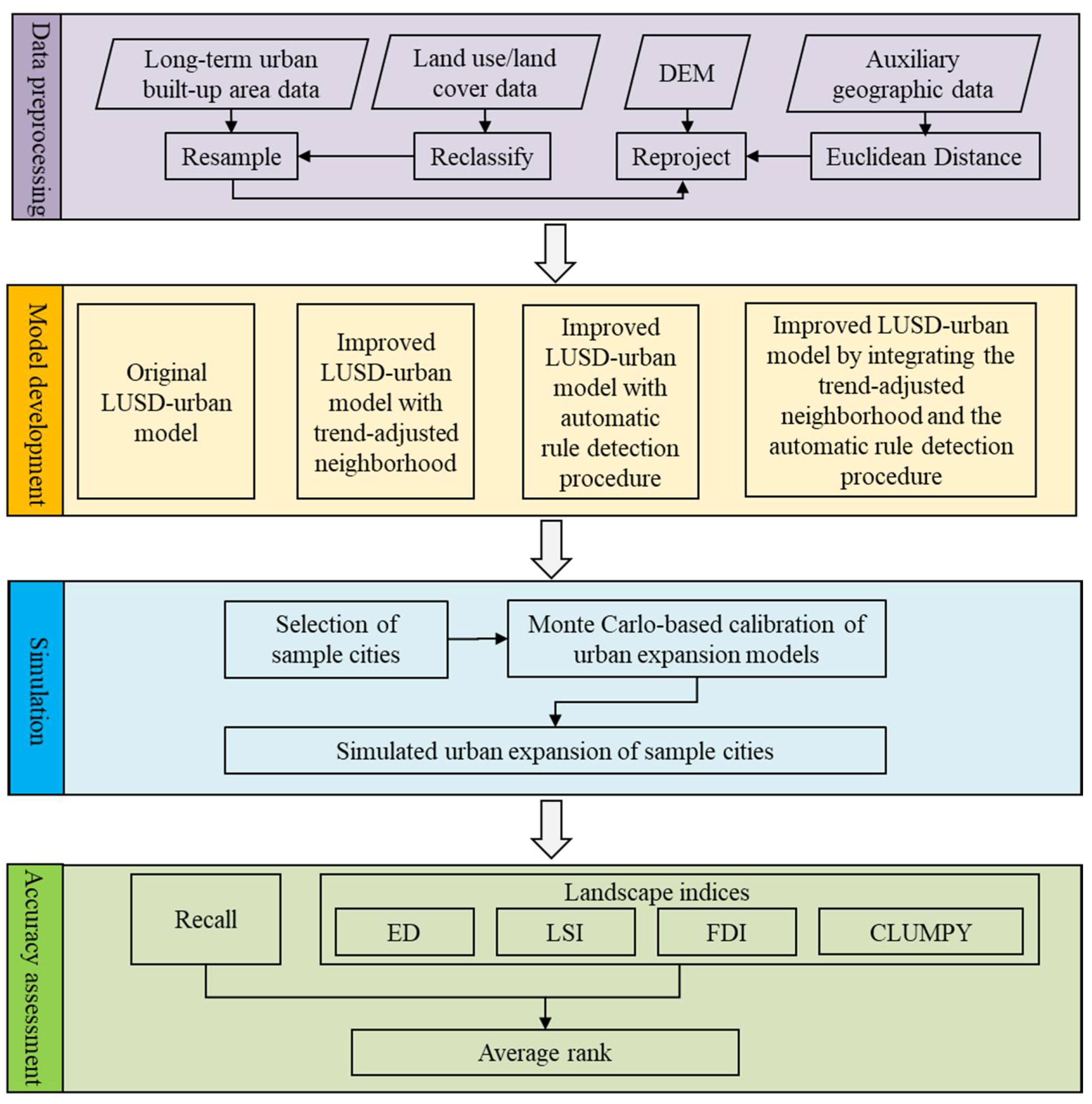
2. Methods
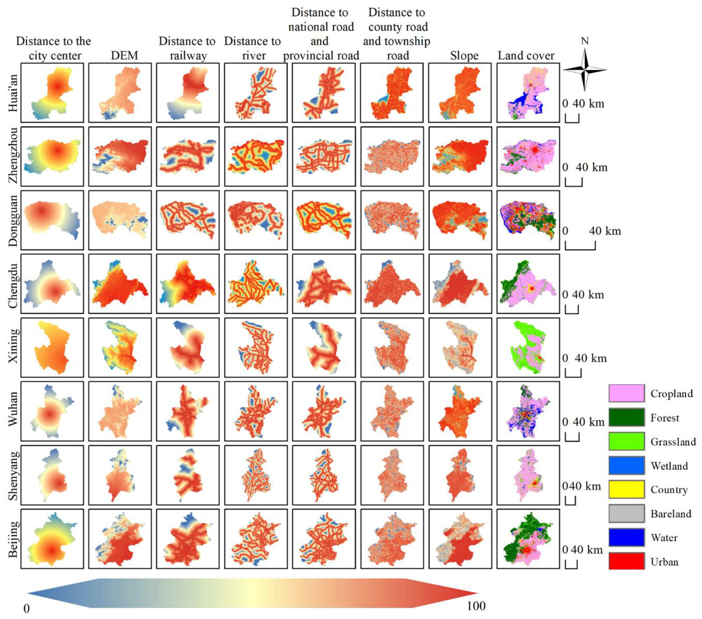
2.1. Data Preprocessing
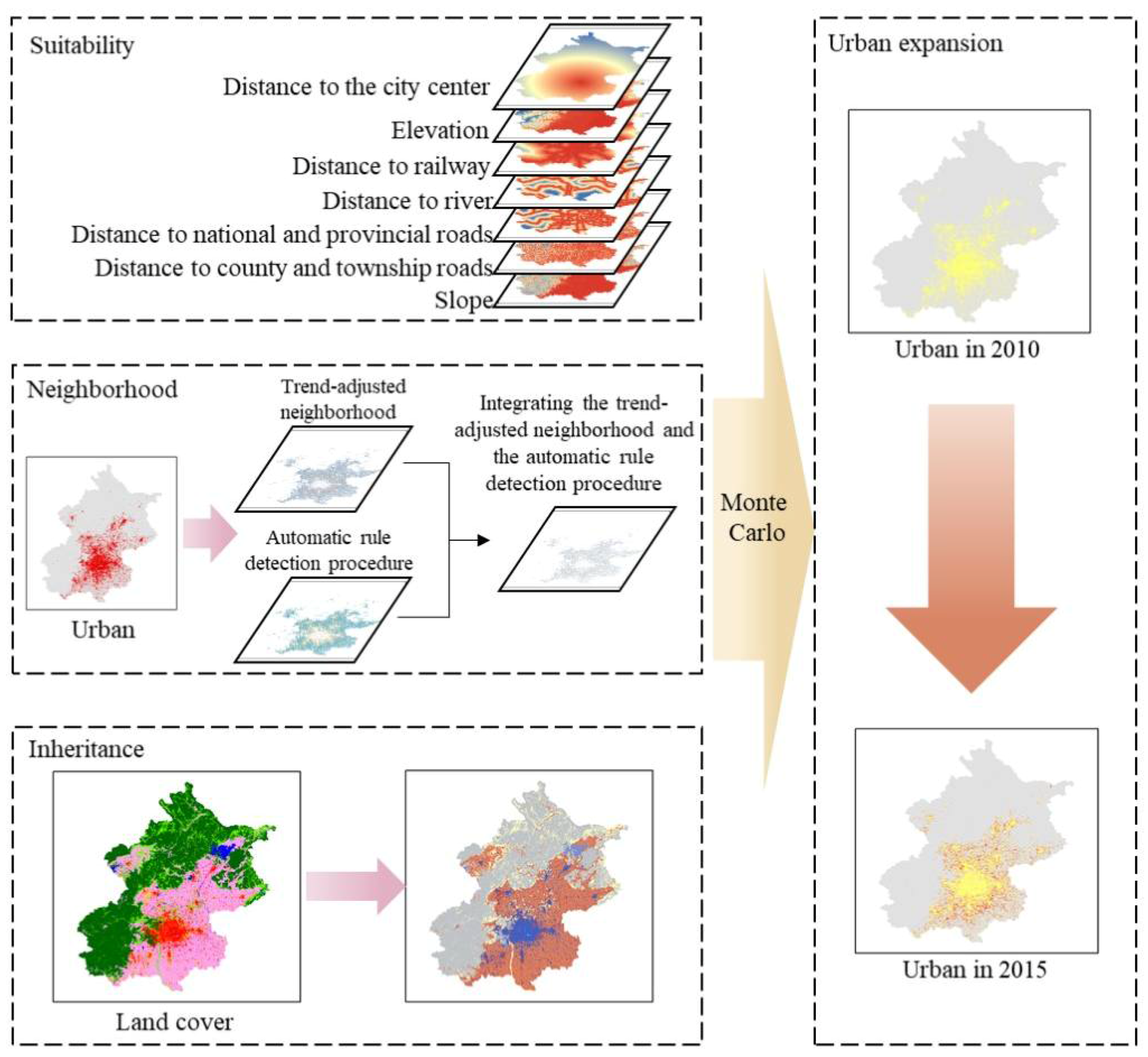
2.2. Model Development
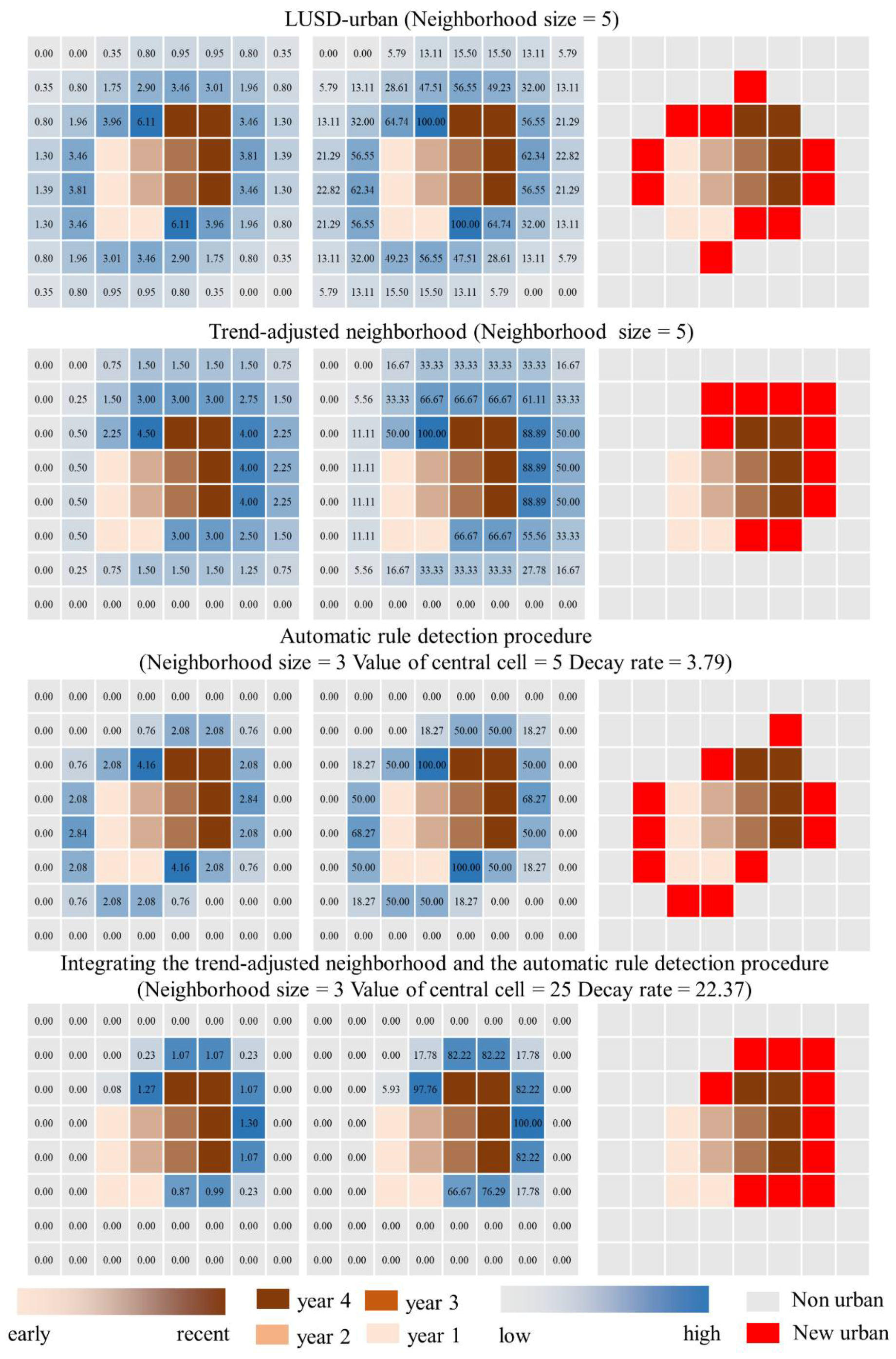
2.2.1. Original LUSD-Urban Model
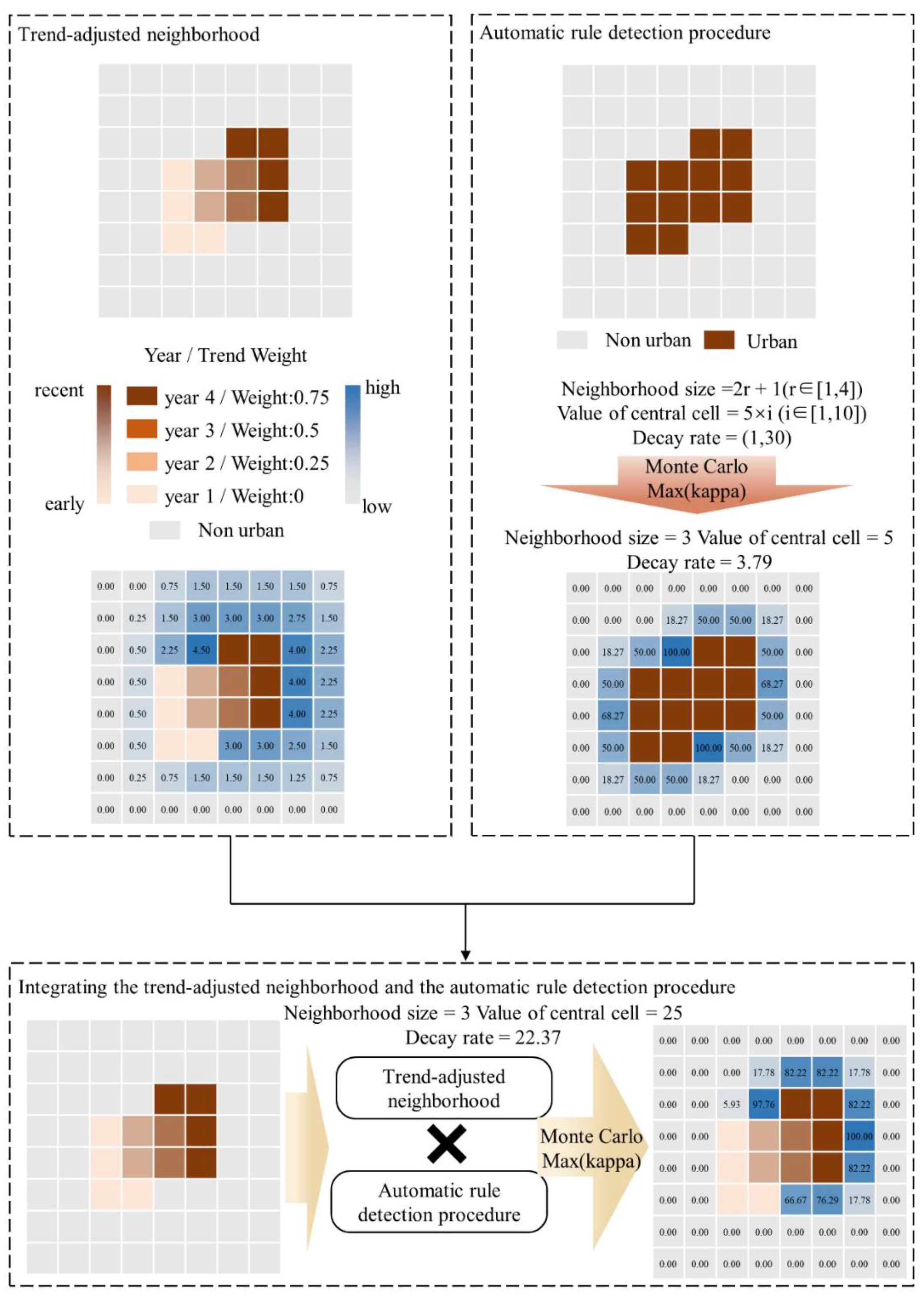
2.2.2. Improved LUSD-Urban Model with Trend-Adjusted Neighborhood
2.2.3. Improved LUSD-Urban Model with Automatic Rule Detection Procedure
2.2.4. Improved LUSD-Urban Model by Integrating the Trend-Adjusted Neighborhood and the Automatic Rule Detection Procedure
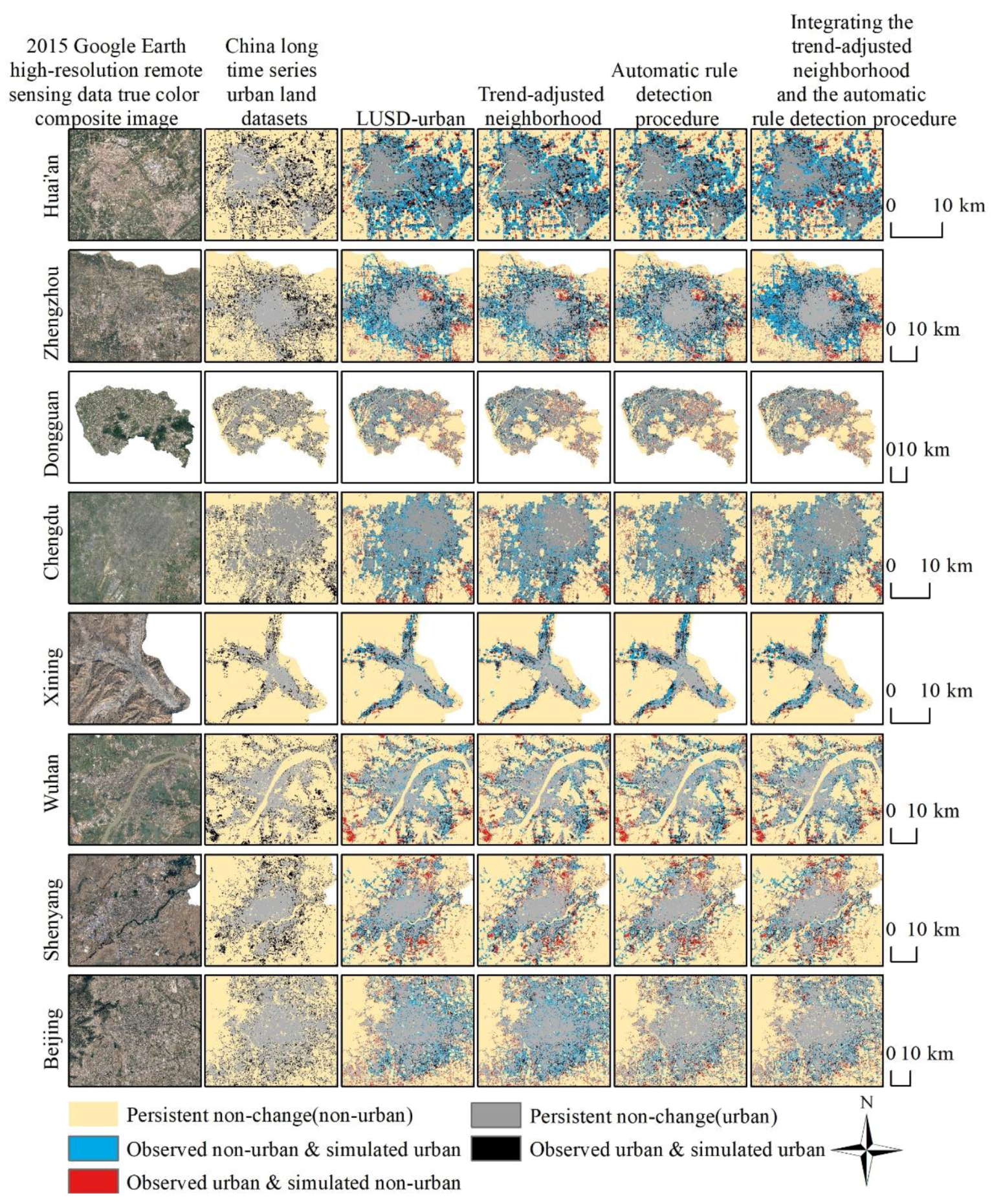
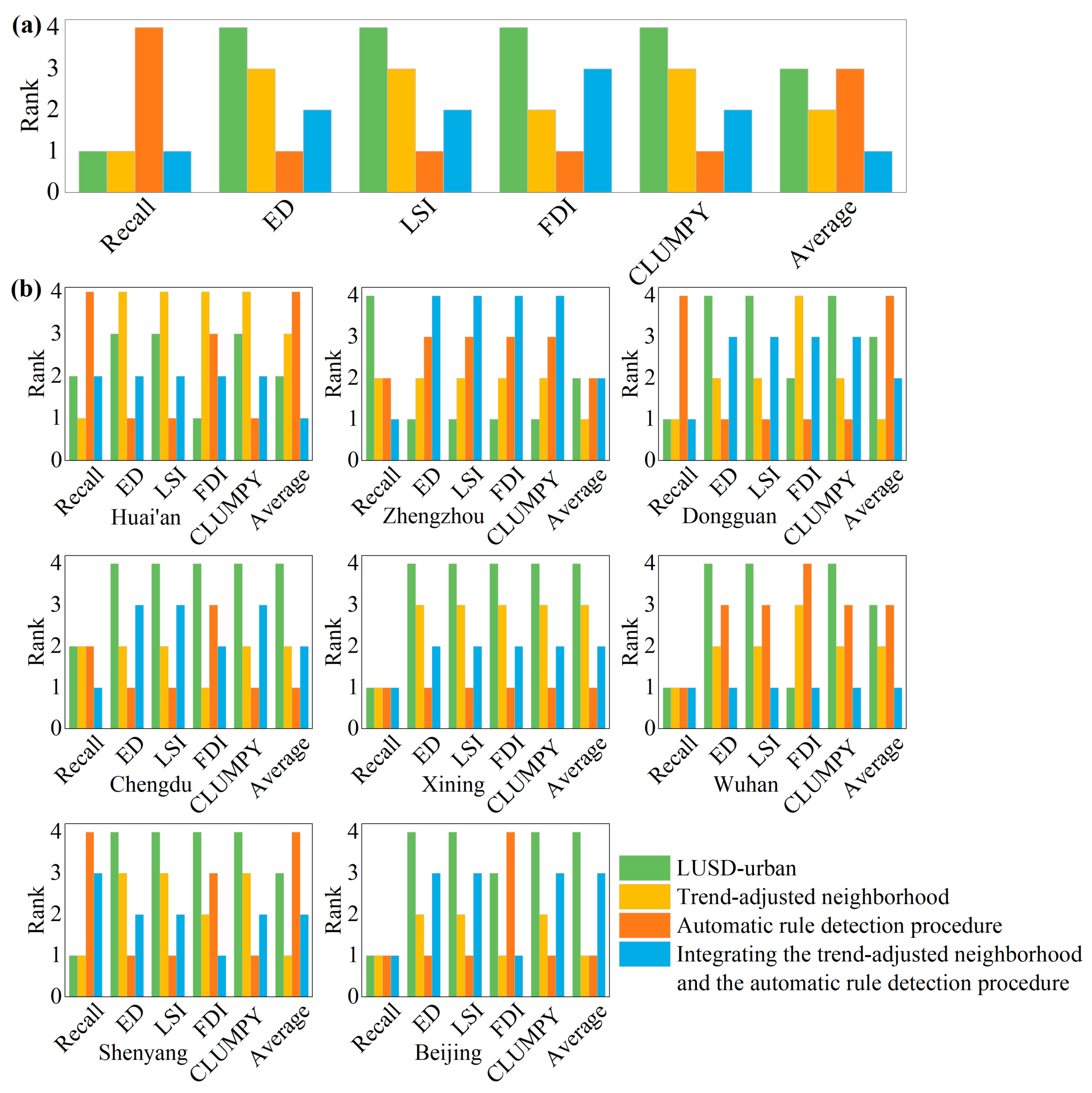
2.3. Simulation and Accuracy Assessment
3. Results
4. Discussion
4.1. Integrating the Trend-Adjusted Neighborhood Algorithm and ARD Procedure Can Increase the Accuracy of Simulated UE
4.2. Future Perspectives
5. Conclusions
Author Contributions
Funding
Institutional Review Board Statement
Informed Consent Statement
Data Availability Statement
Acknowledgments
Conflicts of Interest
Appendix A

| Distance to the City Center | DEM | Distance to Railway | Distance to River | Distance to National and Provincial Roads | Distance to County and Township Roads | Slope | Land Cover | Neighborhood | |
|---|---|---|---|---|---|---|---|---|---|
| Huai’an | 14 | 15 | 1 | 1 | 2 | 11 | 26 | 26 | 4 |
| Zhengzhou | 23 | 4 | 10 | 3 | 11 | 20 | 17 | 11 | 1 |
| Dongguan | 10 | 22 | 1 | 5 | 11 | 25 | 1 | 24 | 1 |
| Chengdu | 4 | 3 | 13 | 3 | 3 | 27 | 2 | 34 | 11 |
| Xining | 21 | 5 | 3 | 9 | 6 | 20 | 22 | 11 | 3 |
| Wuhan | 7 | 7 | 19 | 1 | 1 | 27 | 8 | 26 | 4 |
| Shenyang | 3 | 2 | 3 | 6 | 3 | 28 | 27 | 19 | 9 |
| Beijing | 11 | 22 | 4 | 1 | 18 | 4 | 3 | 11 | 26 |
| Automatic Rule Detection Procedure | Integrating the Trend-Adjusted Neighborhood and the Automatic Rule Detection Procedure | |||||
|---|---|---|---|---|---|---|
| Neighborhood Size | Value of Central Cell | Decay Rate | Neighborhood Size | Value of Central Cell | Decay Rate | |
| Huai’an | 11 | 20 | 28.95 | 11 | 25 | 29.99 |
| Zhengzhou | 11 | 40 | 1.05 | 3 | 40 | 7.14 |
| Dongguan | 11 | 50 | 2.14 | 11 | 40 | 14.50 |
| Chengdu | 5 | 50 | 29.80 | 7 | 15 | 28.87 |
| Xining | 9 | 20 | 29.04 | 11 | 20 | 15.96 |
| Wuhan | 11 | 25 | 1.18 | 11 | 20 | 1.43 |
| Shenyang | 11 | 35 | 6.30 | 11 | 20 | 29.70 |
| Beijing | 5 | 20 | 28.50 | 3 | 30 | 10.51 |
References
- Grimm, N.B.; Faeth, S.H.; Golubiewski, N.E.; Redman, C.L.; Wu, J.G.; Bai, X.M.; Briggs, J.M. Global change and the ecology of cities. Science 2008, 319, 756–760. [Google Scholar] [CrossRef] [PubMed] [Green Version]
- Seto, K.C.; Fragkias, M.; Guneralp, B.; Reilly, M.K. A Meta-Analysis of Global Urban Land Expansion. PLoS ONE 2011, 6, e23777. [Google Scholar] [CrossRef] [PubMed]
- Wu, J.G. Urban ecology and sustainability: The state-of-the-science and future directions. Landsc. Urban Plan. 2014, 125, 209–221. [Google Scholar] [CrossRef]
- Liu, Z.F.; Ding, M.H.; He, C.Y.; Li, J.W.; Wu, J.G. The impairment of environmental sustainability due to rapid urbanization in the dryland region of northern China. Landsc. Urban Plan. 2019, 187, 165–180. [Google Scholar] [CrossRef]
- Pan, X.; Wang, Y.; Liu, Z.; He, C.; Liu, H.; Chen, Z. Understanding Urban Expansion on the Tibetan Plateau over the Past Half Century Based on Remote Sensing: The Case of Xining City, China. Remote Sens. 2020, 13, 46. [Google Scholar] [CrossRef]
- Liu, Z.; He, C.; Yang, Y.; Fang, Z. Planning sustainable urban landscape under the stress of climate change in the drylands of northern China:A scenario analysis based on LUSD-urban model. J. Clean. Prod. 2020, 244, 118709. [Google Scholar] [CrossRef]
- Verburg, P.H.; de Koning, G.H.J.; Kok, K.; Veldkamp, A.; Bouma, J. A spatial explicit allocation procedure for modelling the pattern of land use change based upon actual land use. Ecol. Modell. 1999, 116, 45–61. [Google Scholar] [CrossRef]
- Li, X.; Yeh, A.G.O. Modelling sustainable urban development by the integration of constrained cellular automata and GIS. Int. J. Geogr. Inf. Sci. 2000, 14, 131–152. [Google Scholar] [CrossRef]
- Wu, F.L. Calibration of stochastic cellular automata: The application to rural-urban land conversions. Int. J. Geogr. Inf. Sci. 2002, 16, 795–818. [Google Scholar] [CrossRef]
- Fang, S.F.; Gertner, G.Z.; Sun, Z.L.; Anderson, A.A. The impact of interactions in spatial simulation of the dynamics of urban sprawl. Landsc. Urban Plan. 2005, 73, 294–306. [Google Scholar] [CrossRef]
- He, C.Y.; Okada, N.; Zhang, Q.F.; Shi, P.J.; Li, J.G. Modelling dynamic urban expansion processes incorporating a potential model with cellular automata. Landsc. Urban Plan. 2008, 86, 79–91. [Google Scholar] [CrossRef]
- Sante, I.; Garcia, A.M.; Miranda, D.; Crecente, R. Cellular automata models for the simulation of real-world urban processes: A review and analysis. Landsc. Urban Plan. 2010, 96, 108–122. [Google Scholar] [CrossRef]
- Zhao, L.; Yang, J.; Li, C.; Ge, Y.; Han, Z. Progress on Geographic Cellular Automata Model. Sci. Geogr. Sin. 2016, 36, 1190–1196. [Google Scholar]
- Moreno, N.; Wang, F.; Marceau, D.J. A Geographic Object-based Approach in Cellular Automata Modeling. Photogramm. Eng. Remote Sens. 2010, 76, 183–191. [Google Scholar] [CrossRef]
- Feng, Y.J.; Tong, X.H. Dynamic land use change simulation using cellular automata with spatially nonstationary transition rules. GISci. Remote Sens. 2018, 55, 678–698. [Google Scholar] [CrossRef]
- Hewitt, R.; van Delden, H.; Escobar, F. Participatory land use modelling, pathways to an integrated approach. Environ. Modell. Softw. 2014, 52, 149–165. [Google Scholar] [CrossRef]
- Roodposhti, M.S.; Hewitt, R.J.; Bryan, B.A. Towards automatic calibration of neighbourhood influence in cellular automata land-use models. Comput. Environ. Urban Syst. 2020, 79, 13. [Google Scholar] [CrossRef]
- He, C.Y.; Liu, Z.F.; Tian, J.; Ma, Q. Urban expansion dynamics and natural habitat loss in China: A multiscale landscape perspective. Glob. Change Biol. 2014, 20, 2886–2902. [Google Scholar] [CrossRef]
- He, C.Y.; Okada, N.; Zhang, Q.F.; Shi, P.J.; Zhang, J.S. Modeling urban expansion scenarios by coupling cellular automata model and system dynamic model in Beijing, China. Appl. Geogr. 2006, 26, 323–345. [Google Scholar] [CrossRef]
- Batty, M.; Couclelis, H.; Eichen, M. Urban Systems as Cellular Automata. Environ. Plan. B Plan. Des. 1997, 24, 159–164. [Google Scholar] [CrossRef]
- Wu, F.; Webster, C.J. Simulation of land development through the integration of cellular automata and multicriteria evaluation. Environ. Plan. B Plan. Des. 1998, 25, 103–126. [Google Scholar] [CrossRef]
- Li, X.; Yeh, A.G. Neural-network-based cellular automata for simulating multiple land use changes using GIS. Int. J. Geogr. Inf. Sci. 2002, 16, 323–343. [Google Scholar] [CrossRef]
- Clarke, K.C.; Hoppen, S.; Gaydos, L. A self-modifying cellular automaton model of historical urbanization in the San Francisco Bay area. Environ. Plan. B Plan. Des. 1997, 24, 247–261. [Google Scholar] [CrossRef] [Green Version]
- Verburg, P.H.; Soepboer, W.; Veldkamp, A.; Limpiada, R.; Espaldon, V.; Mastura, S.S.A. Modeling the spatial dynamics of regional land use: The CLUE-S model. Environ. Manag. 2002, 30, 391–405. [Google Scholar] [CrossRef]
- Liu, X.; Liang, X.; Li, X.; Xu, X.; Ou, J.; Chen, Y.; Li, S.; Wang, S.; Pei, F. A future land use simulation model (FLUS) for simulating multiple land use scenarios by coupling human and natural effects. Landsc. Urban Plan. 2017, 168, 94–116. [Google Scholar] [CrossRef]
- Liang, X.; Liu, X.P.; Chen, G.L.; Leng, J.Y.; Wen, Y.Y.; Chen, G.Z. Coupling fuzzy clustering and cellular automata based on local maxima of development potential to model urban emergence and expansion in economic development zones. Int. J. Geogr. Inf. Sci. 2020, 34, 1930–1952. [Google Scholar] [CrossRef]
- Liang, X.; Liu, X.P.; Li, X.; Chen, Y.M.; Tian, H.; Yao, Y. Delineating multi-scenario urban growth boundaries with a CA-based FLUS model and morphological method. Landsc. Urban Plan. 2018, 177, 47–63. [Google Scholar] [CrossRef]
- Couclelis, H. CELLULAR WORLDS—A framework for modeling micro-macro dynamics. Environ. Plan. A 1985, 17, 585–596. [Google Scholar] [CrossRef]
- White, R.; Engelen, G. Cellular automata and fractal urban form: A cellular modelling approach to the evolution of urban land-use patterns. Environ. Plan. A 1993, 25, 1175–1199. [Google Scholar] [CrossRef] [Green Version]
- Batty, M.; Xie, Y. From cells to cities. Environ. Plan. B Plan. Des. 1994, 21, S31–S38. [Google Scholar] [CrossRef]
- Pan, Y.; Roth, A.; Yu, Z.; Doluschitz, R. The impact of variation in scale on the behavior of a cellular automata used for land use change modeling. Comput. Environ. Urban Syst. 2010, 34, 400–408. [Google Scholar] [CrossRef]
- Liao, J.; Tang, L.; Shao, G.; Qiu, Q.; Wang, C.; Zheng, S.; Su, X. A neighbor decay cellular automata approach for simulating urban expansion based on particle swarm intelligence. Int. J. Geogr. Inf. Sci. 2014, 28, 720–738. [Google Scholar] [CrossRef]
- Zhou, Y.Y.; Li, X.C.; Asrar, G.R.; Smith, S.J.; Imhoff, M. A global record of annual urban dynamics (1992–2013) from nighttime lights. Remote Sens. Environ. 2018, 219, 206–220. [Google Scholar] [CrossRef]
- Gong, P.; Li, X.C.; Zhang, W. 40-Year (1978–2017) human settlement changes in China reflected by impervious surfaces from satellite remote sensing. Sci. Bull. 2019, 64, 756–763. [Google Scholar] [CrossRef] [Green Version]
- Huang, X.; Wang, Y.; Li, J.; Chang, X.; Cao, Y.; Xie, J.; Gong, J. High-resolution urban land-cover mapping and landscape analysis of the 42 major cities in China using ZY-3 satellite images. Sci. Bull. 2020, 65, 1039–1048. [Google Scholar] [CrossRef]
- Li, X.C.; Zhou, Y.Y.; Chen, W. An improved urban cellular automata model by using the trend-adjusted neighborhood. Ecol. Process. 2020, 9, 13. [Google Scholar] [CrossRef]
- Tobler, W.R. A Computer Movie Simulating Urban Growth in the Detroit Region. Econ. Geogr. 1970, 46, 234–240. [Google Scholar] [CrossRef]
- Batty, M.; Xie, Y.; Sun, Z. Modeling urban dynamics through GIS-based cellular automata. Comput. Environ. Urban Syst. 1999, 23, 205–233. [Google Scholar] [CrossRef] [Green Version]
- Development Research Center of the State Council PRC. Coordinated Regional Development Strategy and Policy Reports; Development Research Center of the State Council PRC: Beijing, China, 2005.
- Zhang, D.; Huang, Q.X.; He, C.Y.; Wu, J.G. Impacts of urban expansion on ecosystem services in the Beijing-Tianjin-Hebei urban agglomeration, China: A scenario analysis based on the Shared Socioeconomic Pathways. Resour. Conserv. Recycl. 2017, 125, 115–130. [Google Scholar] [CrossRef]
- Fawcett, T. An introduction to ROC analysis. Pattern Recognit. Lett. 2006, 27, 861–874. [Google Scholar] [CrossRef]
- Mcgarigal, K.S.; Cushman, S.; Neel, M.; Ene, E. Fragstats: Spatial Pattern Analysis Program for Categorical Maps; Version 4.2; University of Massachusetts: Amherst, MA, USA, 2002. [Google Scholar]
- Chen, Y.; Li, X.; Liu, X.; Ai, B. Modeling urban land-use dynamics in a fast developing city using the modified logistic cellular automaton with a patch-based simulation strategy. Int. J. Geogr. Inf. Sci. 2014, 28, 234–255. [Google Scholar] [CrossRef]

| Name | Classifications/Variables | Year | Spatial Resolution/Accuracy | Data Source/Reference/Hyperlink |
|---|---|---|---|---|
| Long-term urban built-up area data | Urban built-up area data | 1985, 1990, 1995, 2000, 2010 and 2015 | Spatial resolution: 30 m Kappa coefficient: above 0.90 | The dataset of urban land in China (Gong et al., 2019) (http://data.ess.tsinghua.edu.cn/, accessed on 10 November 2020) |
| Land use/land cover data | Cropland, forest, grassland, wetland, rural construction land, bare land, water, and urban | 2000 | Spatial resolution: 30 m Kappa coefficient: 0.79 | GlobalLand30 product (http://www.globallandcover.com/, accessed on 10 November 2020) |
| Digital elevation model | Spatial resolution: 30 m | Geospatial Data Cloud Platform of the Computer Network Information Center of the Chinese Academy of Sciences (http://www.gscloud.cn, accessed on 10 November 2020) | ||
| Auxiliary geographic data | Administrative boundary data, urban center points, roads, and rivers | National Basic Geographic Information Center (http://ngcc.sbsm.gov.cn/, accessed on 10 November 2020) |
| Model | Recall | ED | LSI | FDI | CLUMPY | Final Rank | ||||||
|---|---|---|---|---|---|---|---|---|---|---|---|---|
| Recall | Rank | Score | Rank | Score | Rank | Score | Rank | Score | Rank | |||
| Huai’an | LUSD-urban | 0.68 | 2 | 1.40 | 3 | 32.91 | 3 | 0.0021 | 1 | 0.1580 | 3 | 2 |
| TN 1 | 0.70 | 1 | 1.44 | 4 | 33.92 | 4 | 0.0037 | 4 | 0.1629 | 4 | 3 | |
| ARDP 2 | 0.66 | 4 | 1.15 | 1 | 27.16 | 1 | 0.0032 | 3 | 0.1304 | 1 | 4 | |
| ITN&ARDP 3 | 0.68 | 2 | 1.32 | 2 | 31.10 | 2 | 0.0029 | 2 | 0.1493 | 2 | 1 | |
| Zhengzhou | LUSD-urban | 0.75 | 4 | 5.18 | 1 | 35.77 | 1 | 0.0040 | 1 | 0.1041 | 1 | 2 |
| TN 1 | 0.76 | 2 | 5.63 | 2 | 38.82 | 2 | 0.0048 | 2 | 0.1130 | 2 | 1 | |
| ARDP 2 | 0.76 | 2 | 5.65 | 3 | 39.00 | 3 | 0.0049 | 3 | 0.1135 | 3 | 2 | |
| ITN&ARDP 3 | 0.77 | 1 | 5.84 | 4 | 40.28 | 4 | 0.0073 | 4 | 0.1172 | 4 | 2 | |
| Dongguan | LUSD-urban | 0.89 | 1 | 4.98 | 4 | 13.88 | 4 | 0.0017 | 2 | 0.0578 | 4 | 3 |
| TN 1 | 0.89 | 1 | 4.78 | 2 | 13.32 | 2 | 0.0022 | 4 | 0.0554 | 2 | 1 | |
| ARDP 2 | 0.88 | 4 | 4.36 | 1 | 12.17 | 1 | 0.0016 | 1 | 0.0506 | 1 | 4 | |
| ITN&ARDP 3 | 0.89 | 1 | 4.80 | 3 | 13.38 | 3 | 0.0021 | 3 | 0.0557 | 3 | 2 | |
| Chengdu | LUSD-urban | 0.79 | 2 | 1.61 | 4 | 38.28 | 4 | 0.0017 | 4 | 0.1453 | 4 | 4 |
| TN 1 | 0.79 | 2 | 1.44 | 2 | 34.43 | 2 | 0.0013 | 1 | 0.1308 | 2 | 2 | |
| ARDP 2 | 0.79 | 2 | 1.38 | 1 | 32.81 | 1 | 0.0016 | 3 | 0.1246 | 1 | 1 | |
| ITN&ARDP 3 | 0.80 | 1 | 1.49 | 3 | 35.57 | 3 | 0.0015 | 2 | 0.1350 | 3 | 2 | |
| Xining | LUSD-urban | 0.77 | 1 | 1.05 | 4 | 23.03 | 4 | 0.0118 | 4 | 0.1664 | 4 | 4 |
| TN 1 | 0.77 | 1 | 0.95 | 3 | 20.82 | 3 | 0.0093 | 3 | 0.1504 | 3 | 3 | |
| ARDP 2 | 0.77 | 1 | 0.91 | 1 | 19.98 | 1 | 0.0082 | 1 | 0.1444 | 1 | 1 | |
| ITN&ARDP 3 | 0.77 | 1 | 0.93 | 2 | 20.38 | 2 | 0.0084 | 2 | 0.1473 | 2 | 2 | |
| Wuhan | LUSD-urban | 0.74 | 1 | 2.58 | 4 | 41.95 | 4 | 0.0002 | 1 | 0.1451 | 4 | 3 |
| TN 1 | 0.74 | 1 | 2.36 | 2 | 38.40 | 2 | 0.0005 | 3 | 0.1328 | 2 | 2 | |
| ARDP 2 | 0.74 | 1 | 2.40 | 3 | 39.17 | 3 | 0.0006 | 4 | 0.1355 | 3 | 3 | |
| ITN&ARDP 3 | 0.74 | 1 | 2.21 | 1 | 36.06 | 1 | 0.0002 | 1 | 0.1247 | 1 | 1 | |
| Shenyang | LUSD-urban | 0.77 | 1 | 1.41 | 4 | 30.50 | 4 | 0.0025 | 4 | 0.1074 | 4 | 3 |
| TN 1 | 0.77 | 1 | 1.34 | 3 | 29.06 | 3 | 0.0020 | 2 | 0.1023 | 3 | 1 | |
| ARDP 2 | 0.75 | 4 | 1.14 | 1 | 24.58 | 1 | 0.0023 | 3 | 0.0865 | 1 | 4 | |
| ITN&ARDP 3 | 0.76 | 3 | 1.26 | 2 | 27.13 | 2 | 0.0019 | 1 | 0.0955 | 2 | 2 | |
| Beijing | LUSD-urban | 0.84 | 1 | 2.74 | 4 | 40.46 | 4 | 0.0008 | 3 | 0.0845 | 4 | 4 |
| TN 1 | 0.84 | 1 | 2.36 | 2 | 34.80 | 2 | 0.0004 | 1 | 0.0727 | 2 | 1 | |
| ARDP 2 | 0.84 | 1 | 2.34 | 1 | 34.50 | 1 | 0.0009 | 4 | 0.0721 | 1 | 1 | |
| ITN&ARDP 3 | 0.84 | 1 | 2.41 | 3 | 35.66 | 3 | 0.0004 | 1 | 0.0745 | 3 | 3 | |
| Average | LUSD-urban | 0.78 | 1 | 2.62 | 4 | 32.10 | 4 | 0.0031 | 4 | 0.1211 | 4 | 3 |
| TN 1 | 0.78 | 1 | 2.54 | 3 | 30.45 | 3 | 0.0030 | 2 | 0.1150 | 3 | 2 | |
| ARDP 2 | 0.77 | 4 | 2.42 | 1 | 28.67 | 1 | 0.0029 | 1 | 0.1072 | 1 | 3 | |
| ITN&ARDP 3 | 0.78 | 1 | 2.53 | 2 | 29.95 | 2 | 0.0031 | 3 | 0.1124 | 2 | 1 | |
Publisher’s Note: MDPI stays neutral with regard to jurisdictional claims in published maps and institutional affiliations. |
© 2021 by the authors. Licensee MDPI, Basel, Switzerland. This article is an open access article distributed under the terms and conditions of the Creative Commons Attribution (CC BY) license (https://creativecommons.org/licenses/by/4.0/).
Share and Cite
Pan, X.; Wang, Z.; Huang, M.; Liu, Z. Improving an Urban Cellular Automata Model Based on Auto-Calibrated and Trend-Adjusted Neighborhood. Land 2021, 10, 688. https://doi.org/10.3390/land10070688
Pan X, Wang Z, Huang M, Liu Z. Improving an Urban Cellular Automata Model Based on Auto-Calibrated and Trend-Adjusted Neighborhood. Land. 2021; 10(7):688. https://doi.org/10.3390/land10070688
Chicago/Turabian StylePan, Xinhao, Zichen Wang, Miao Huang, and Zhifeng Liu. 2021. "Improving an Urban Cellular Automata Model Based on Auto-Calibrated and Trend-Adjusted Neighborhood" Land 10, no. 7: 688. https://doi.org/10.3390/land10070688
APA StylePan, X., Wang, Z., Huang, M., & Liu, Z. (2021). Improving an Urban Cellular Automata Model Based on Auto-Calibrated and Trend-Adjusted Neighborhood. Land, 10(7), 688. https://doi.org/10.3390/land10070688