
Combining Site Characterization, Monitoring and Hydromechanical Modeling for Assessing Slope Stability

 , , ,
, , ,  , and
, and 
Abstract
1. Introduction
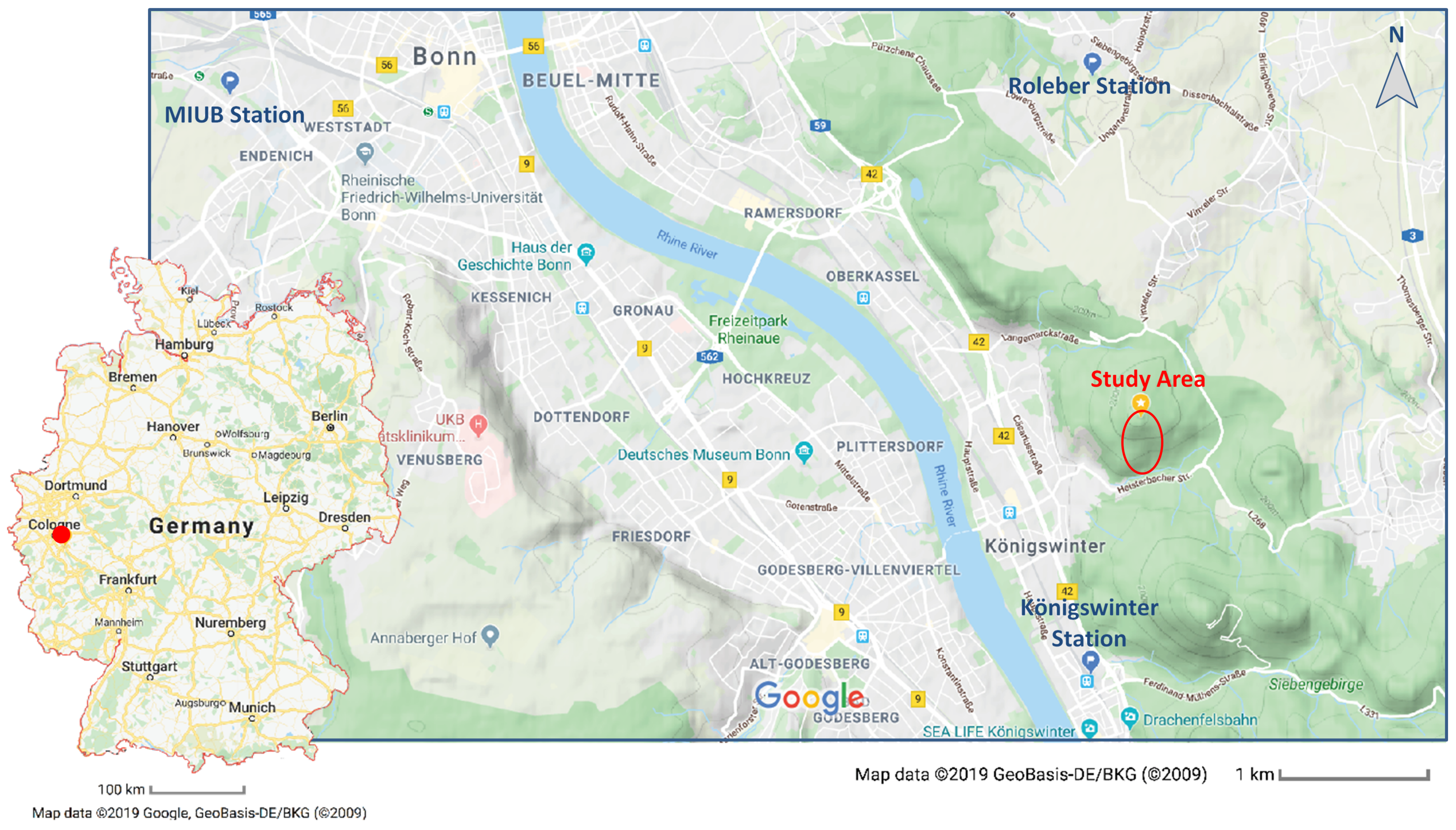
2. Study Area
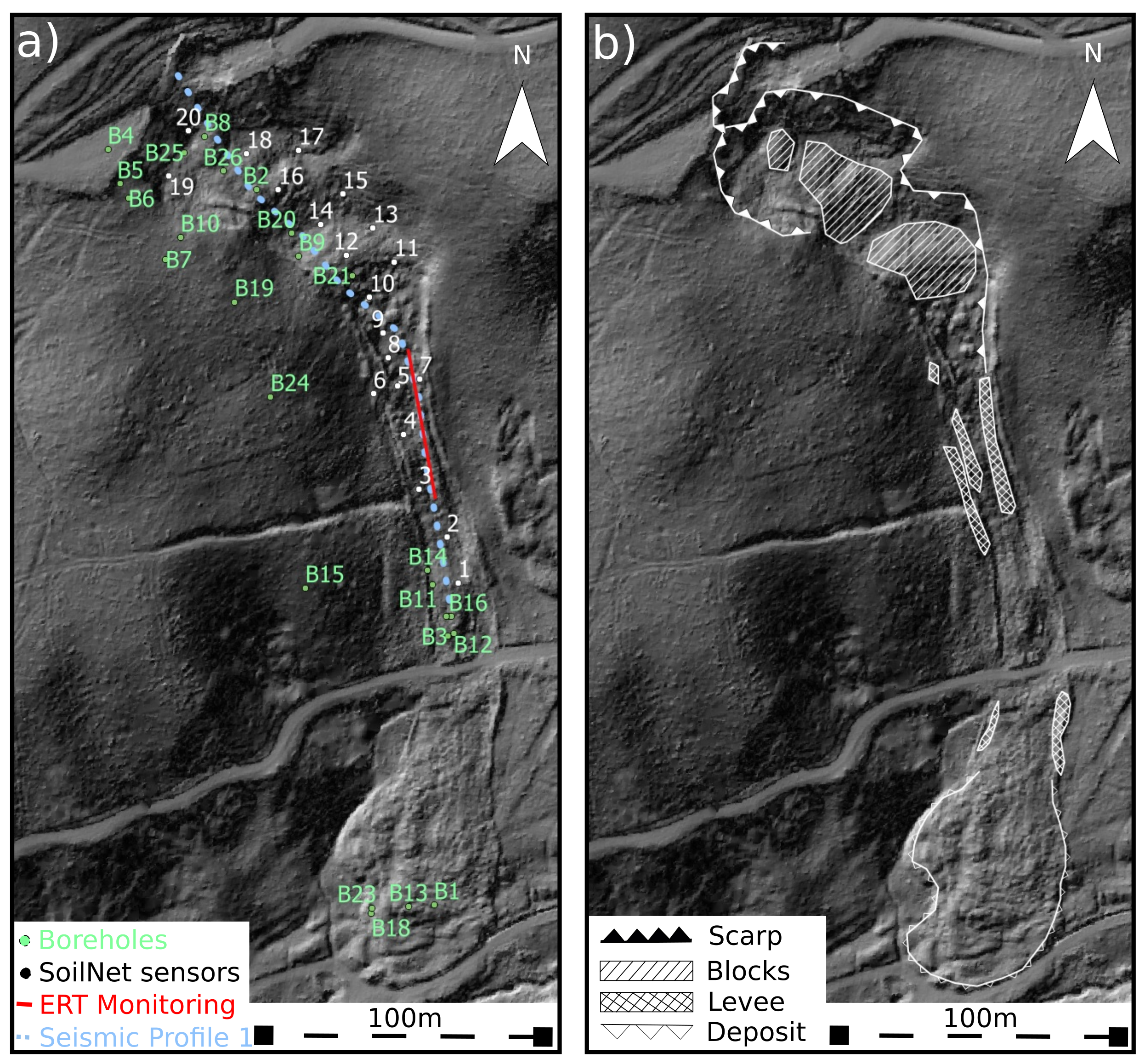
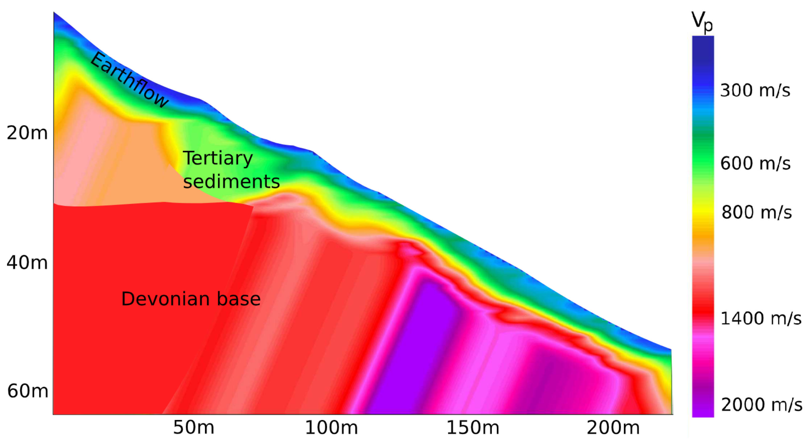
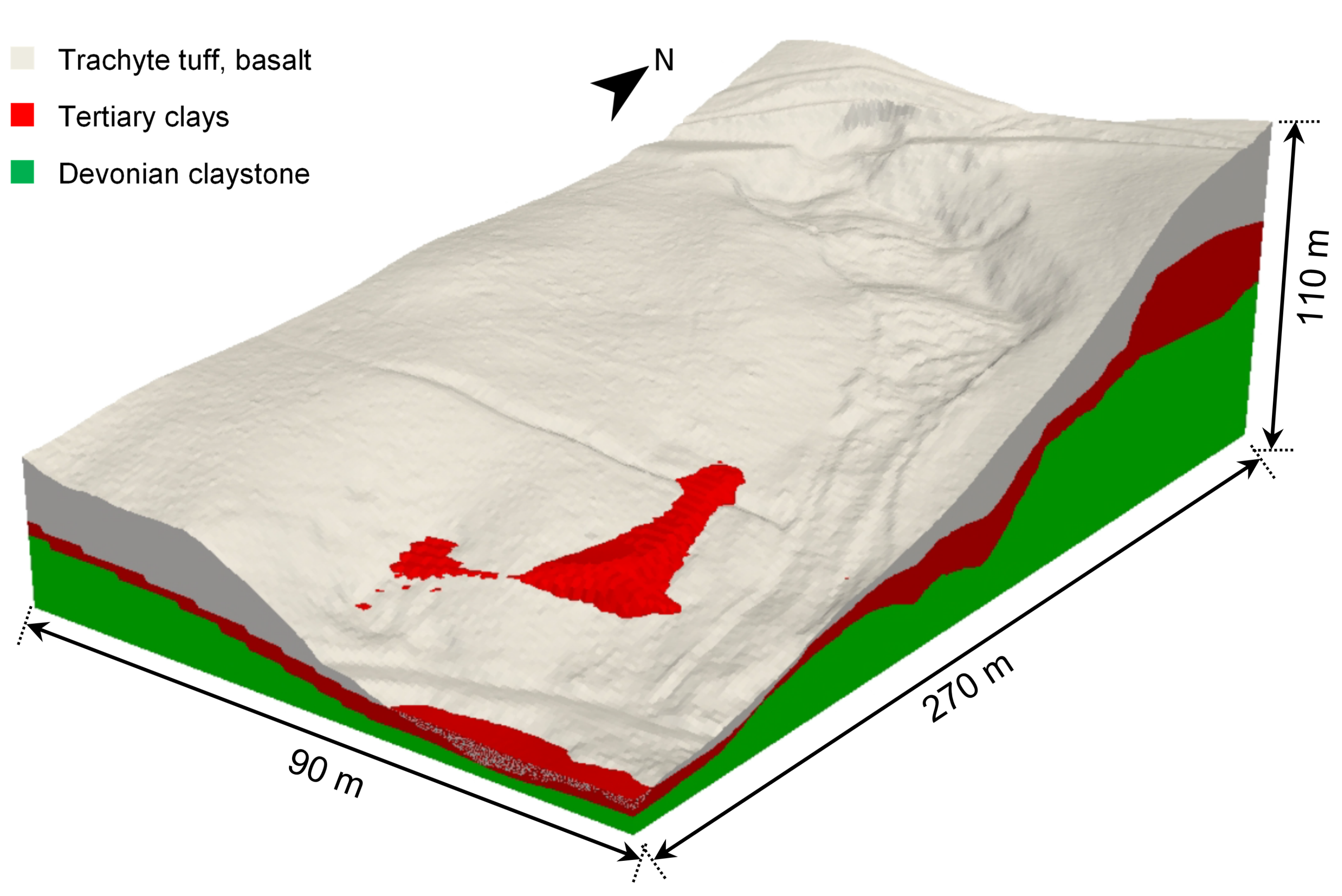
2.1. Site Characterization
- a top layer consisting of clayey sediments, trachyte tuff and loess, transported and mixed by the landslides;
- an intermediate layer of Tertiary sediments mainly consisting of silt and clay;
- a base layer of Devonian bedrock, strongly weathered at the top.
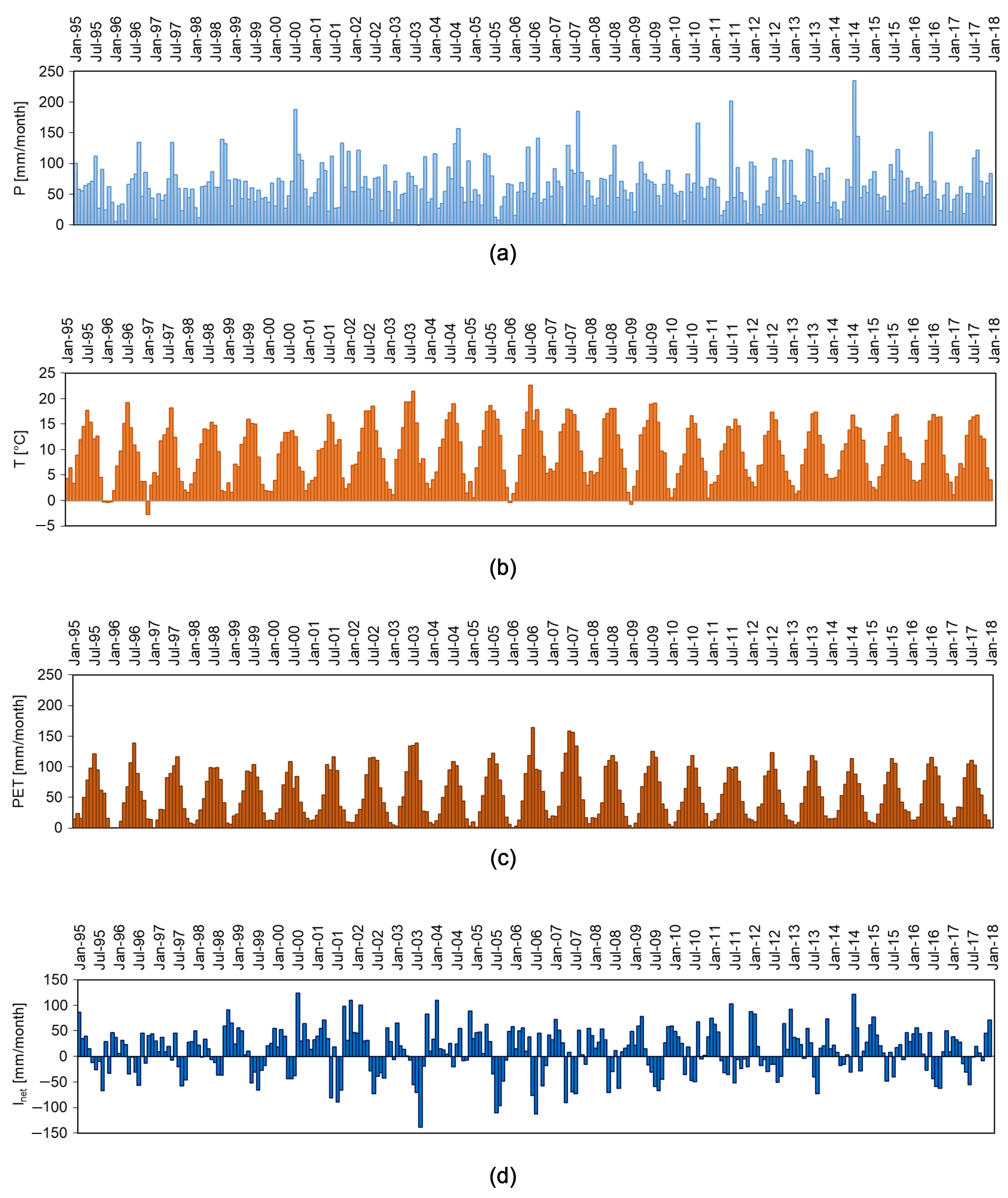
2.2. Meteorological Data
2.3. Monitoring of Ground Water Level and Soil Water Content
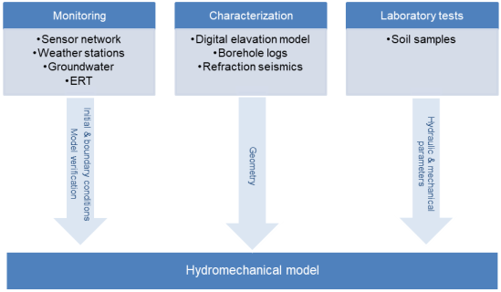
3. Hydromechanical Model
4. Combination of Field Observations and Hydromechanical Modeling
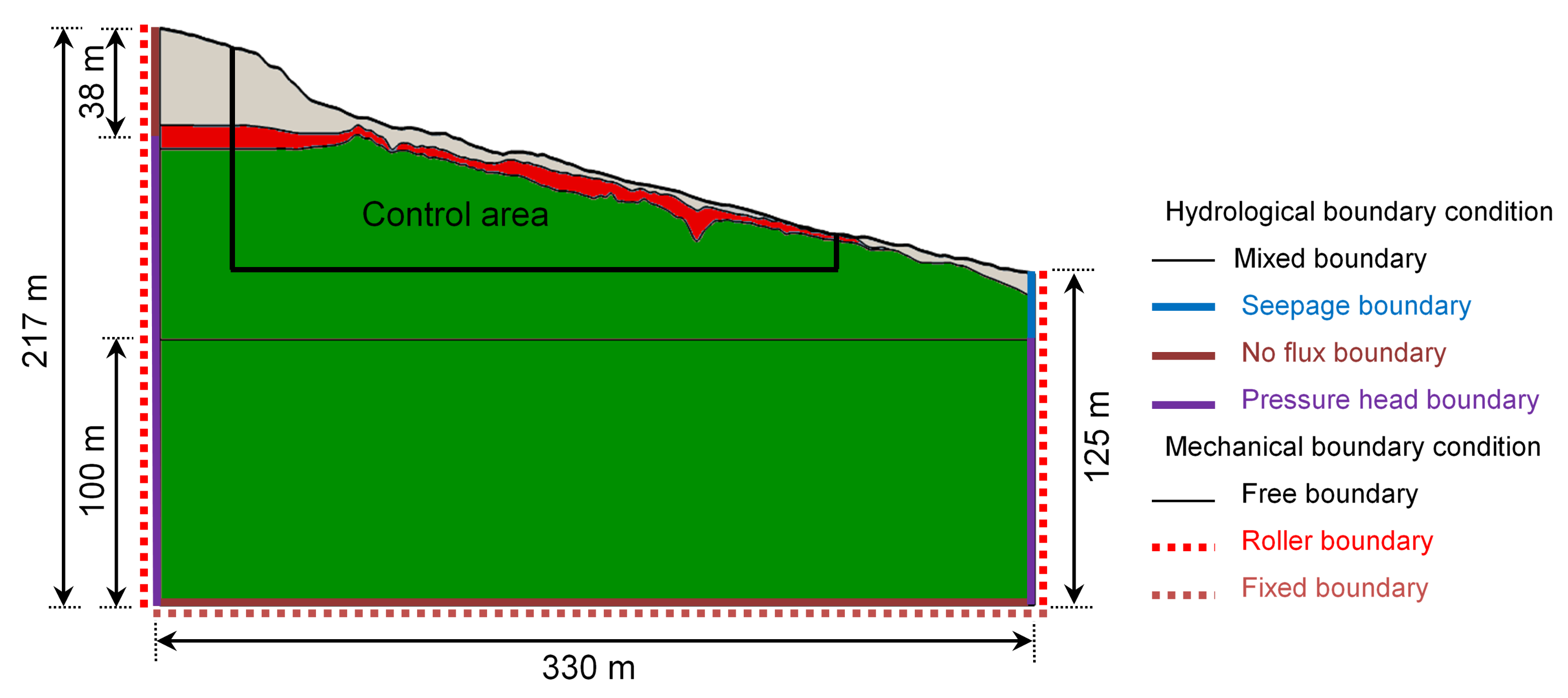
4.1. Model Setup
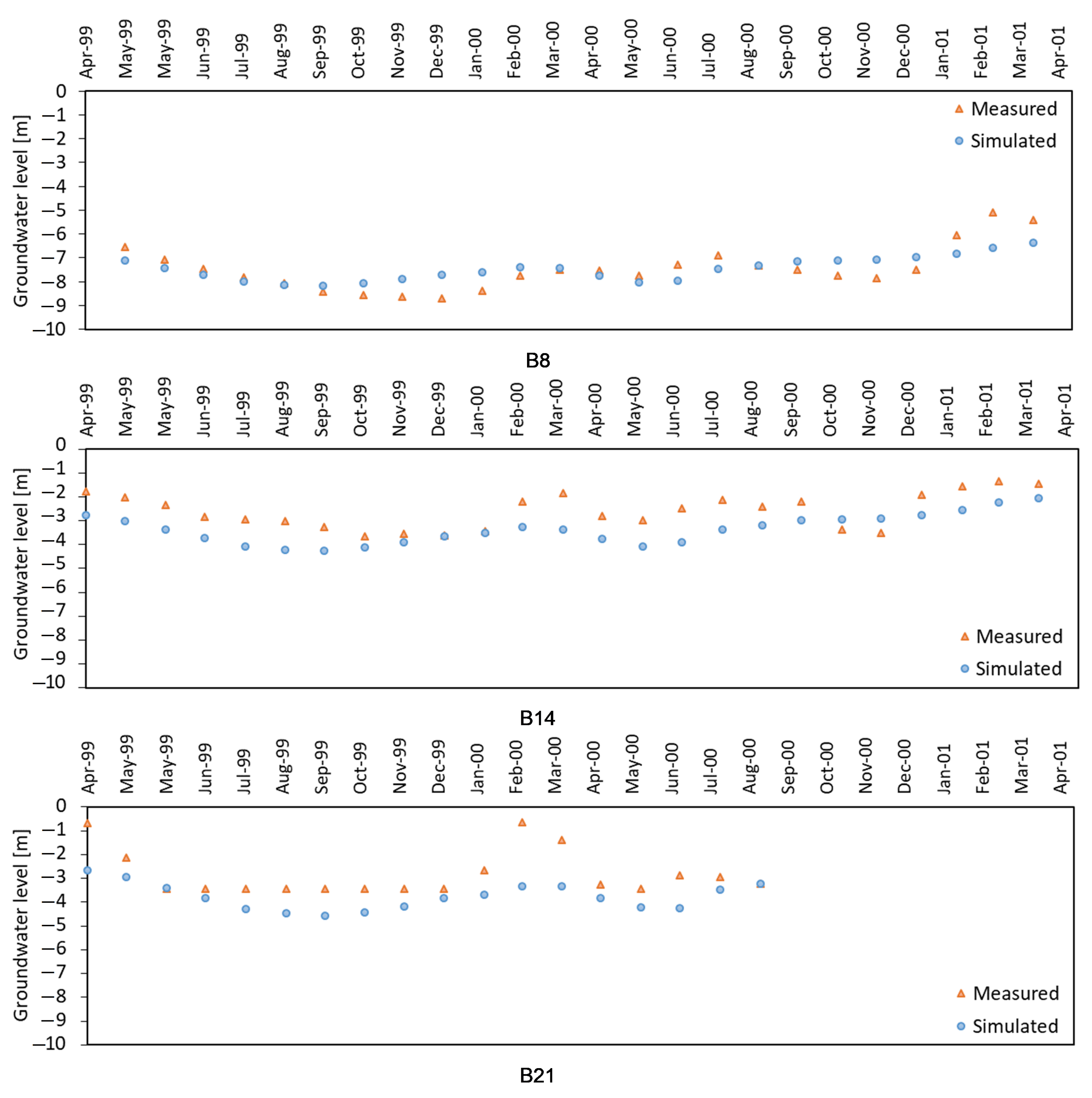
4.2. Model Calibration and Validation
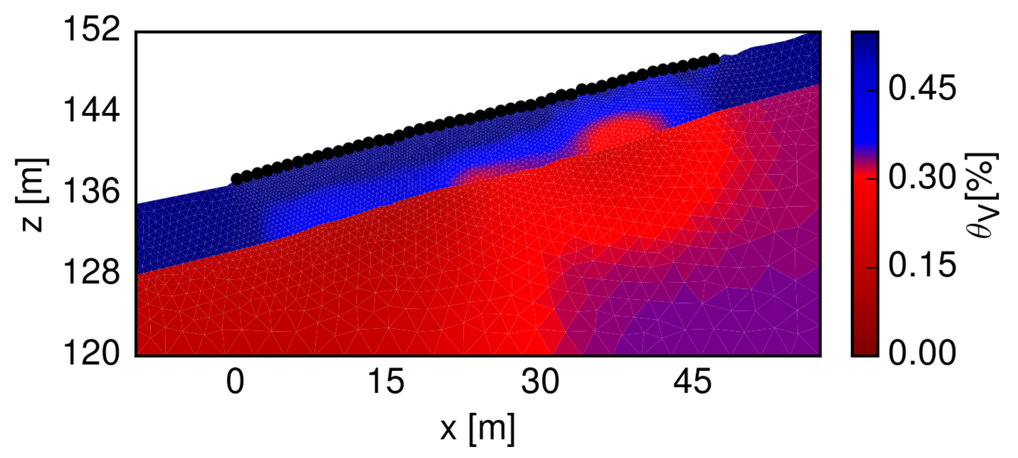
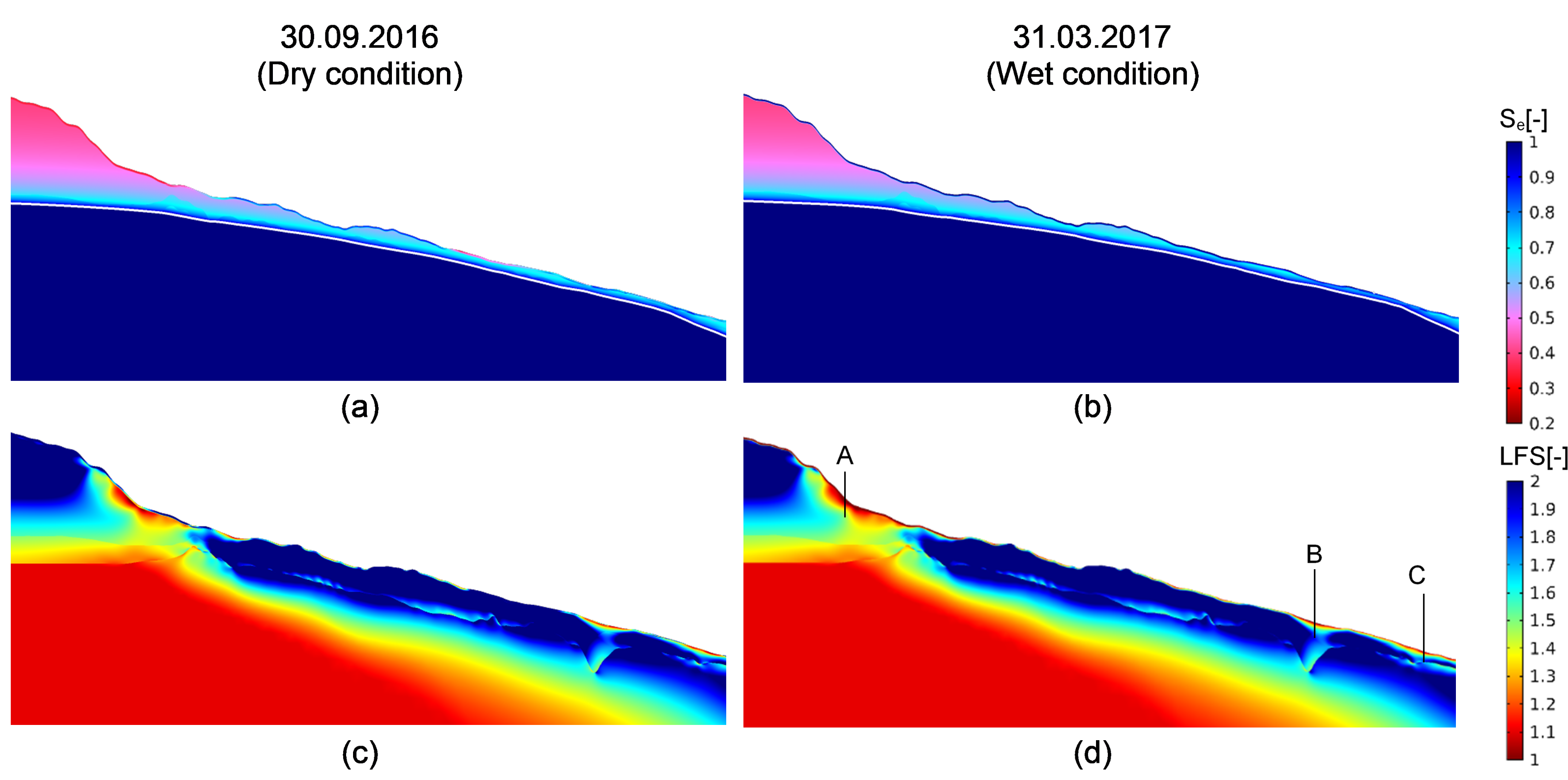
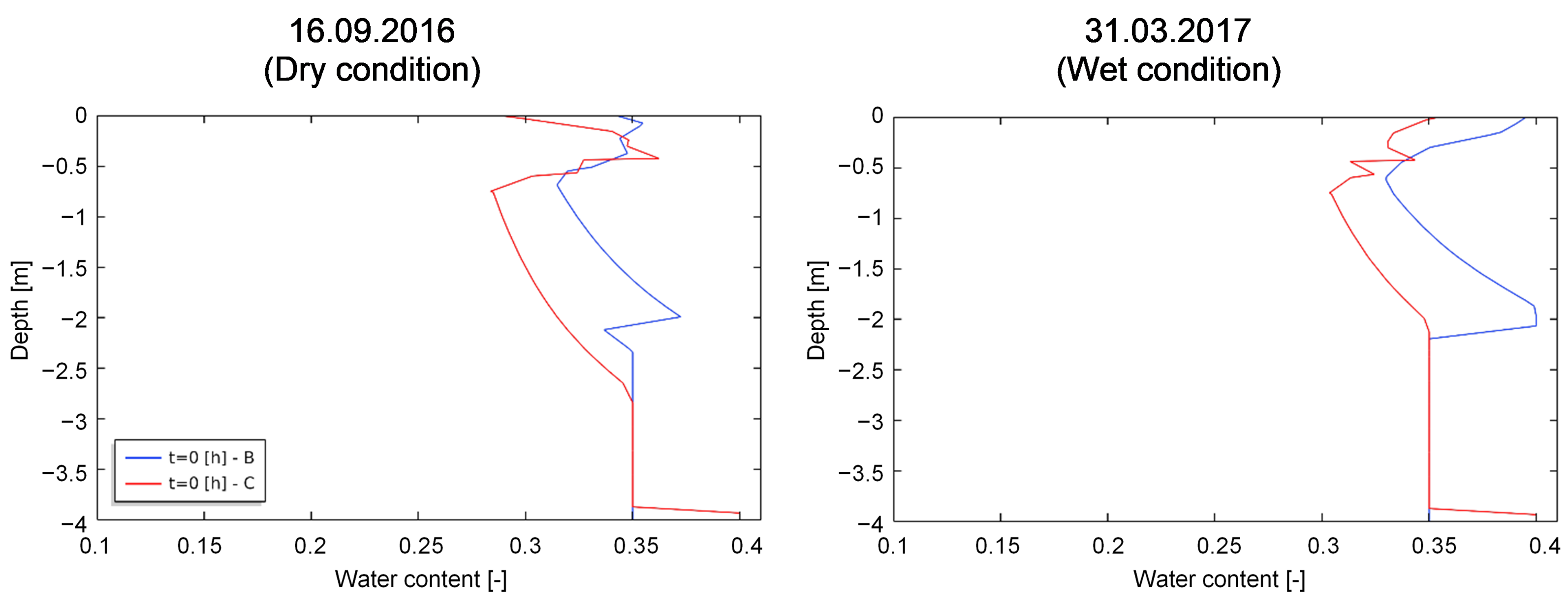
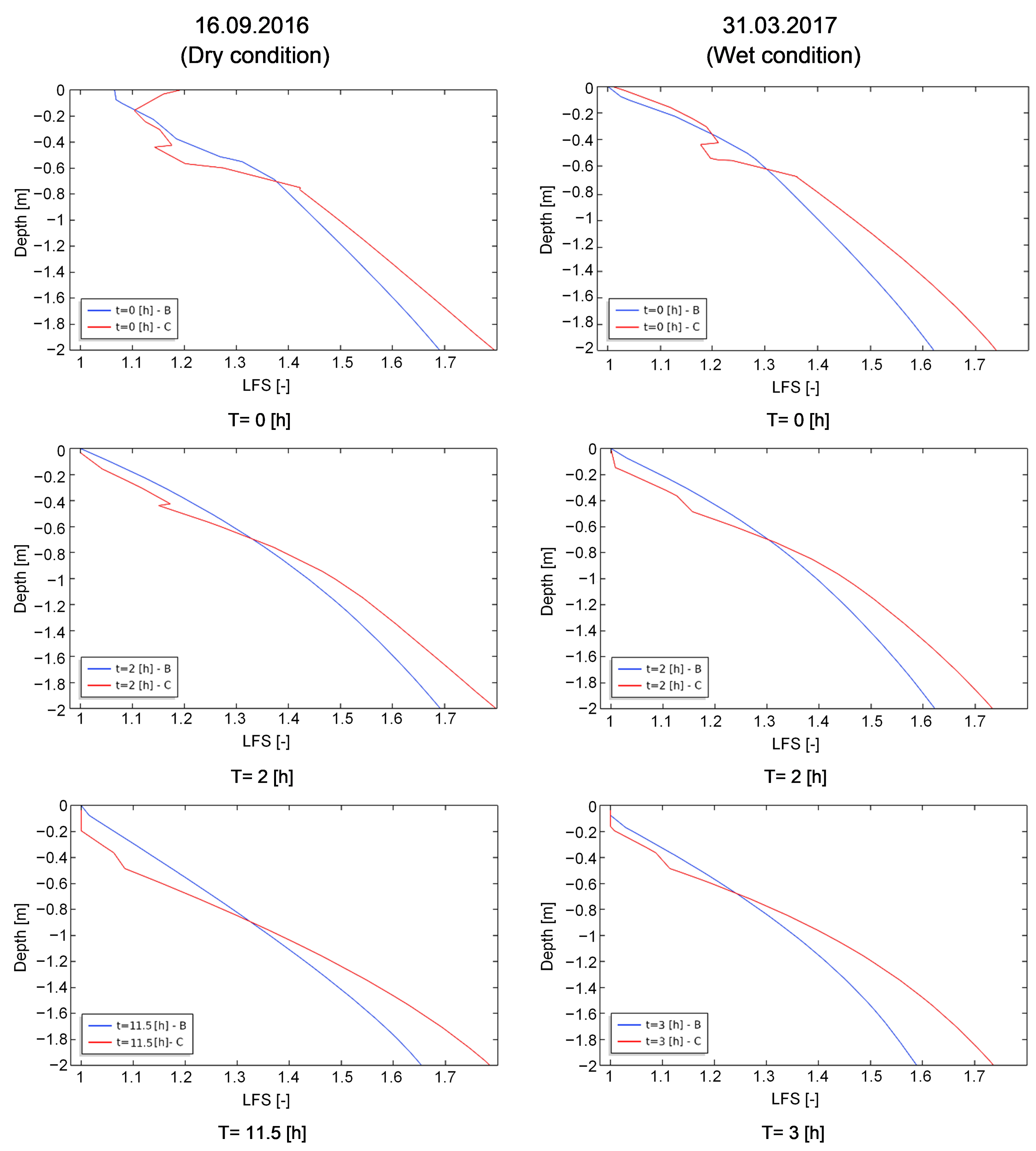
5. Model Results for Precipitation Events
6. Discussion
7. Conclusions
Author Contributions
Funding
Institutional Review Board Statement
Informed Consent Statement
Data Availability Statement
Acknowledgments
Conflicts of Interest
Abbreviations
| LFS | Local factor of safety |
| ERT | Electrical resistivity tomography |
| MIUB | Department of Meteorology of the University of Bonn |
| PET | Potential evapotranspiration |
References
- Jakob, M.; Lambert, S. Climate change effects on landslides along the southwest coast of British Columbia. Geomorphology 2009, 107, 275–284. [Google Scholar] [CrossRef]
- Petley, D.N. On the impact of climate change and population growth on the occurrence of fatal landslides in South, East and SE Asia. Q. J. Eng. Geol. Hydrogeol. 2010, 43, 487–496. [Google Scholar] [CrossRef]
- Saez, J.L.; Corona, C.; Stoffel, M.; Berger, F. Climate change increases frequency of shallow spring landslides in the French Alps. Geology 2013, 41, 619–622. [Google Scholar] [CrossRef]
- Lu, N.; Godt, J. Infinite slope stability under steady unsaturated seepage conditions. Water Resour. Res. 2008, 44. [Google Scholar] [CrossRef]
- Lu, N.; Sener-Kaya, B.; Wayllace, A.; Godt, J.W. Analysis of rainfall-induced slope instability using a field of local factor of safety. Water Resour. Res. 2012, 48, 1–14. [Google Scholar] [CrossRef]
- Liu, Q.Q.; Li, J.C. Effects of Water Seepage on the Stability of Soil-slopes. Procedia IUTAM 2015, 17, 29–39. [Google Scholar] [CrossRef]
- Rabie, M. Comparison study between traditional and finite element methods for slopes under heavy rainfall. HBRC J. 2014, 10, 160–168. [Google Scholar] [CrossRef]
- Stianson, J.; Chan, D.; Fredlund, D. Role of Admissibility Criteria in Limit Equilibrium Slope Stability Methods Based on Finite Element Stresses. Comput. Geotech. 2015, 66, 113–125. [Google Scholar] [CrossRef]
- Lanni, C.; McDonnell, J.; Hopp, L.; Rigon, R. Simulated effect of soil depth and bedrock topography on near-surface hydrologic response and slope stability. Earth Surf. Process. Landforms 2013, 38, 146–159. [Google Scholar] [CrossRef]
- Reid, M.E.; Iverson, R.M. Gravity-driven groundwater-flow and slope failure potential. 2. Effects of slope morphology, material properies, and hydraulic heterogeneity. Water Resour. Res. 1992, 28, 939–950. [Google Scholar] [CrossRef]
- Kim, M.S.; Onda, Y.; Kim, J.K.; Kim, S.W. Effect of topography and soil parameterisation representing soil thicknesses on shallow landslide modelling. Quat. Int. 2015, 384, 91–106. [Google Scholar] [CrossRef]
- Tromp-van Meerveld, H.J.; McDonnell, J.J. On the interrelations between topography, soil depth, soil moisture, transpiration rates and species distribution at the hillslope scale. Adv. Water Resour. 2006, 29, 293–310. [Google Scholar] [CrossRef]
- Moradi, S.; Huisman, J.; Class, H.; Vereecken, H. The effect of bedrock topography on timing and location of landslide initiation using the local factor of safety concept. Water 2018, 10, 1290. [Google Scholar] [CrossRef]
- Lapenna, V.; Lorenzo, P.; Perrone, A.; Piscitelli, S.; Sdao, F.; Rizzo, E. High-resolution geoelectrical tomographies in the study of Giarrossa landslide (Southern Italy). Bull. Eng. Geol. Environ. 2003, 62, 259–268. [Google Scholar] [CrossRef]
- Sass, O.; Bell, R.; Glade, T. Comparison of GPR, 2D-resistivity and traditional techniques for the subsurface exploration of the Öschingen landslide, Swabian Alb (Germany). Geomorphology 2008, 93, 89–103. [Google Scholar] [CrossRef]
- Jongmans, D.; Bievre, G.; Renalier, F.; Schwartz, S.; Beaurez, N.; Orengo, Y. Geophysical investigation of a large landslide in glaciolacustrine clays in the Trieves area (French Alps). Eng. Geol. 2009, 109, 45–56. [Google Scholar] [CrossRef]
- Gance, J.; Malet, J.P.; Supper, R.; Sailhac, P.; Ottowitz, D.; Jochum, B. Permanent electrical resistivity measurements for monitoring water circulation in clayey landslides. J. Appl. Geophys. 2016, 126, 98–115. [Google Scholar] [CrossRef]
- Uhlemann, S.; Chambers, J.; Wilkinson, P.; Maurer, H.; Merritt, A.; Meldrum, P.; Kuras, O.; Gunn, D.; Smith, A.; Dijkstra, T. 4D imaging of moisture dynamics during landslide reactivation. J. Geophys. Res. Earth Surf. 2016. [Google Scholar] [CrossRef]
- Göktürkler, G.; Balkaya, C.; Erhan, Z. Geophysical investigation of a landslide: The Altindag landslide site, Izmir (Western Turkey). J. Appl. Geophys. 2008, 65, 84–96. [Google Scholar] [CrossRef]
- Chambers, J.E.; Wilkinson, P.B.; Kuras, O.; Ford, J.R.; Gunn, D.A.; Meldrum, P.I.; Pennington, C.V.L.; Weller, A.L.; Hobbs, P.R.N.; Ogilvy, R.D. Three-dimensional geophysical anatomy of an active landslide in Lias Group mudrocks, Cleveland Basin, UK. Geomorphology 2011, 125, 472–484. [Google Scholar] [CrossRef]
- Mauritsch, H.J.; Seiberl, W.; Arndt, R.; Römer, A.; Schneiderbauer, K.; Sendlhofer, G.P. Geophysical investigations of large landslides in the Carnic region of southern Austria. Eng. Geol. 2000, 56, 373–388. [Google Scholar] [CrossRef]
- Glade, T.; Stark, P.; Dikau, R. Determination of potential landslide shear plane depth using seismic refraction—A case study in Rheinhessen, Germany. Bull. Eng. Geol. Environ. 2005, 64, 151–158. [Google Scholar] [CrossRef]
- Baron, I.; Supper, R. Application and reliability of techniques for landslide site investigation, monitoring and early warning- Outcomes from a questionnaire study. Nat. Hazards Earth Syst. Sci. 2013, 13, 3157–3168. [Google Scholar] [CrossRef]
- Lehmann, P.; Gambazzi, F.; Suski, B.; Baron, L.; Askarinejad, A.; Springman, S.M.; Holliger, K.; Or, D. Evolution of soil wetting patterns preceding a hydrologically induced landslide inferred from electrical resistivity survey and point measurements of volumetric water content and pore water pressure. Water Resour. Res. 2013, 49, 7992–8004. [Google Scholar] [CrossRef]
- Archie, G.E. The electrical resistivity log as an aid in determining some reservoir characteristics. Trans. AIME 1942, 146, 54–62. [Google Scholar] [CrossRef]
- Waxman, M.H.; Smits, L.J.M. Electrical conductivities in oil-bearing shaly sands. Soc. Pet. Eng. J. 1968, 8, 107–122. [Google Scholar] [CrossRef]
- Hübner, R.; Heller, K.; Günther, T.; Kleber, A. Monitoring Hillslope Moisture Dynamics with Surface ERT for Enhancing Spatial Significance of Hydrometric Point Measurements. Hydrol. Earth Syst. Sci. 2015, 19, 225–240. [Google Scholar] [CrossRef]
- Hibert, C.; Grandjean, G.; Bitri, A.; Travelletti, J.; Malet, J.P. Characterizing Landslides through Geophysical Data Fusion: Example of the La Valette Landslide (France). Eng. Geol. 2012, 128, 23–29. [Google Scholar] [CrossRef]
- Hojat, A.; Arosio, D.; Ivanov, V.I.; Longoni, L.; Papini, M.; Scaioni, M.; Tresoldi, G.; Zanzi, L. Geoelectrical Characterization and Monitoring of Slopes on a Rainfall-Triggered Landslide Simulator. J. Appl. Geophys. 2019, 170, 103844. [Google Scholar] [CrossRef]
- Heinze, T.; Limbrock, J.; Pudasaini, S.; Kemna, A. Relating Mass Movement with Electrical Self-Potential Signals. Geophys. J. Int. 2019, 216, 55–60. [Google Scholar] [CrossRef]
- Whiteley, J.S.; Chambers, J.E.; Uhlemann, S.; Wilkinson, P.B.; Kendall, J.M. Geophysical Monitoring of Moisture-Induced Landslides: A Review. Rev. Geophys. 2019, 57, 106–145. [Google Scholar] [CrossRef]
- Bogena, H.R.; Herbst, M.; Huisman, J.A.; Rosenbaum, U.; Weuthen, A.; Vereecken, H. Potential of wireless sensor networks for measuring soil water content variability. Vadose Zone J. 2010, 9, 1002–1013. [Google Scholar] [CrossRef]
- Srinivasan, K.; Howell, B.; Anderson, E.; Flores, A. A low cost wireless sensor network for landslide hazard monitoring. In Proceedings of the 2012 IEEE International Geoscience and Remote Sensing Symposium (IGARSS), Munich, Germany, 22–27 July 2012. [Google Scholar]
- Piegari, E.; Cataudella, V.; Di Maio, R.; Milano, L.; Nicodemi, M.; Soldovieri, M.G. Electrical resistivity tomography and statistical analysis in landslide modelling: A conceptual approach. J. Appl. Geophys. 2009, 68, 151–158. [Google Scholar] [CrossRef]
- Tric, E.; Lebourg, T.; Jomard, H.; Le Cossec, J. Study of Large-Scale Deformation Induced by Gravity on the La Clapière Landslide (Saint-Etienne de Tinée, France) Using Numerical and Geophysical Approaches. J. Appl. Geophys. 2010, 70, 206–215. [Google Scholar] [CrossRef]
- Ling, C.; Xu, Q.; Zhang, Q.; Ran, J.; Lv, H. Application of electrical resistivity tomography for investigating the internal structure of a translational landslide and characterizing its groundwater circulation (Kualiangzi landslide, Southwest China). J. Appl. Geophys. 2016, 131, 154–162. [Google Scholar] [CrossRef]
- Pasierb, B.; Grodecki, M.; Gwóźdź, R. Geophysical and Geotechnical Approach to a Landslide Stability Assessment: A Case Study. Acta Geophys. 2019, 67, 1823–1834. [Google Scholar] [CrossRef]
- Schmidt, J. The Role of Mass Movements for Slope Evolution. Ph.D. Thesis, Universitäts-und Landesbibliothek Bonn, Bonn, Germany, 2001. [Google Scholar]
- Hardenbicker, U. Hangrutschungen im Bonner Raum-Naturraeumliche Einordnung und ihre Anthropogenen Ursachen; Ferdinand Dümmlers Verlag: Bonn, Germany, 1994. [Google Scholar]
- García, A.; Hördt, A.; Fabian, M. Landslide monitoring with high resolution tilt measurements at the Dollendorfer Hardt landslide, Germany. Geomorphology 2010, 120, 16–25. [Google Scholar] [CrossRef]
- Schmidt, J.; Dikau, R. Preparatory and triggering factors for slope failure: Analyses of two landslides near Bonn, Germany. Z. Geomorphol. 2005, 49, 121–138. [Google Scholar]
- Weber, M. Welchen Beitrag kann die Luftbildinterpretation zur Erfassung und Datierung von Hangrutschungen leisten – Erste Ergebnisse aus dem Bonner Raum. Arb. Zur Rheinischen Landeskd. 1991, 60, 19–30. [Google Scholar]
- Reynolds, J.M. An Introduction to Applied and Environmental Geophysics; Wiley: Chichester, UK, 1997. [Google Scholar]
- Schön, J.H. Physical Propoperties of Rocks; Elsevier: Amsterdam, The Netherlands, 2011. [Google Scholar]
- Thornthwaite, C.W. An Approach toward a Rational Classification of Climate. Geogr. Rev. 1948, 38, 55–94. [Google Scholar] [CrossRef]
- Schrödter, H. Verdunstung: Anwendungsorientierte Meßverfahren und Bestimmungsmethoden; Springer: Berlin, Germany, 1985. [Google Scholar]
- Xiang, K.Y.; Li, Y.; Horton, R.; Feng, H. Similarity and difference of potential evapotranspiration and reference crop evapotranspiration—A review. Agric. Water Manag. 2020, 232, 1–16. [Google Scholar] [CrossRef]
- Bogena, H.R.; Huisman, J.A.; Schilling, B.; Weuthen, A.; Vereecken, H. Effective calibration of low-cost soil water content sensors. Sensors 2017, 17, 208. [Google Scholar] [CrossRef]
- Roth, K.; Schulin, R.; Fluhler, H.; Attinger, W. Calibration of time domain reflectometry for water content measurement using a composite dielectric approach. Water Resour. Res. 1990, 26, 2267–2273. [Google Scholar] [CrossRef]
- Robinson, D.A.; Jones, S.B.; Blonquist, J.M.; Friedman, S.P. A physically derived water content/permittivity calibration model for coarse-textured, layered soils. Soil Sci. Soc. Am. J. 2005, 69, 1372–1378. [Google Scholar] [CrossRef]
- Hayley, K.; Bentley, L.R.; Gharibi, M.; Nightingale, M. Low temperature dependence of electrical resistivity: Implications for near surface geophysical monitoring. Geophys. Res. Lett. 2007, 34, L18402. [Google Scholar] [CrossRef]
- Brunet, P.; Clément, R.; Bouvier, C. Monitoring soil water content and deficit using Electrical Resistivity Tomography (ERT)—A case study in the Cevennes area, France. J. Hydrol. 2010, 380, 146–153. [Google Scholar] [CrossRef]
- Kemna, A. Tomographic Inversion of Complex Resistivity. Ph.D. Thesis, Ruhr-Universität Bochum, Bochum, Germany, 2000. [Google Scholar]
- Slater, L.; Binley, A.; Daily, W.; Johnson, R. Cross-hole electrical imaging of a controlled saline tracer injection. J. Appl. Geophys. 2000, 44, 85–102. [Google Scholar] [CrossRef]
- Günther, T.; Rücker, C. A New Joint Inversion Approach Applied to the Combined Tomography of DC Resistivity and Seismic Refraction Data. In Symposium on the Application of Geophysics to Engineering and Environmental Problems 2006; Society of Exploration Geophysicists: Tulsa, OK, USA, 2006; pp. 1196–1202. [Google Scholar] [CrossRef]
- Doetsch, J.; Linde, N.; Pessognelli, M.; Green, A.G.; Günther, T. Constraining 3-D electrical resistance tomography with GPR reflection data for improved aquifer characterization. J. Appl. Geophys. 2012, 78, 68–76. [Google Scholar] [CrossRef]
- Nguyen, F.; Kemna, A. Strategies for Time-Lapse Electrical Resistivity Inversion. In Near Surface Geoscience 2005 11th European Meeting of Environmental and Engineering Geophysics; European Association of Geoscientists and Engineers: Houten, The Netherlands, 2005; p. A005. [Google Scholar] [CrossRef]
- Rhoades, J.D.; Manteghi, N.A.; Shouse, P.J.; Alves, W.J. Soil Electrical Conductivity and Soil Salinity: New Formulations and Calibrations. Soil Sci. Soc. Am. J. 1989, 53, 433. [Google Scholar] [CrossRef]
- Gillis, G.; Pirie, G. Schlumberger Oilfield Glossary—Geophysics Module. 2018. Available online:https://www.glossary.oilfield.slb.com (accessed on 15 October 2018).
- Van Genuchten, M.T. A Closed-form Equation for Predicting the Hydraulic Conductivity of Unsaturated Soils1. Soil Sci. Soc. Am. J. 1980, 44, 892. [Google Scholar] [CrossRef]
- Lu, N.; Likos, W.J. Suction stress characteristic curve for unsaturated soil. J. Geotech. Geoenviron. Eng. 2006, 132, 131–142. [Google Scholar] [CrossRef]
- Lu, N.; Godt, J.W.; Wu, D.T. A closed-form equation for effective stress in unsaturated soil. Water Resour. Res. 2010, 46, 1–14. [Google Scholar] [CrossRef]
- DIN. Baugrund, Untersuchung von Bodenproben—Bestimmung der Dichte des Bodens (DIN 18125); Deutsches Institut für Normung e.V. (DIN): Berlin, Germany, 1993. [Google Scholar]
- DIN. Baugrund, Versuche und Versuchsgeräte—Bestimmung des Wasseraufnahmevermögens (DIN 18132); Deutsches Institut für Normung e.V. (DIN): Berlin, Germany, 1993. [Google Scholar]
- DIN. Baugrund, Untersuchung von Bodenproben—Bestimmung des Wasserdurchlässigkeitsbeiwerts (DIN 18130); Deutsches Institut für Normung e.V. (DIN): Berlin, Germany, 1993. [Google Scholar]
- DIN. Baugrund, Untersuchung von Bodenproben—Bestimmung der Scherfestigkeit (DIN 18137); Deutsches Institut für Normung e.V. (DIN): Berlin, Germany, 1993. [Google Scholar]
- Schaap, M.G.; Leij, F.J.; van Genuchten, M.T. ROSETTA: A computer program for estimating soil hydraulic parameters with hierarchical pedotransfer functions. J. Hydrol. 2001, 251, 163–176. [Google Scholar] [CrossRef]
- Kezdi, A. Handbook of Soil Mechanics; Elsevier: Amsterdam, The Netherlands, 1980. [Google Scholar]
- Obrzud, R.; Truty, A. The Hardening Soil Model—A Practical Guidbook; Z_Soil.PC 100701 Report; Zace Services: Lausanne, Switzerland, 2018. [Google Scholar]
- Stahli, M.; Sattele, M.; Huggel, C.; McArdell, B.W.; Lehmann, P.; Van Herwijnen, A.; Berne, A.; Schleiss, M.; Ferrari, A.; Kos, A.; et al. Monitoring and prediction in early warning systems for rapid mass movements. Nat. Hazards Earth Syst. Sci. 2015, 15, 905–917. [Google Scholar] [CrossRef]
- Greco, R.; Pagano, L. Basic features of the predictive tools of early warning systems for water-related natural hazards: Examples for shallow landslides. Nat. Hazards Earth Syst. Sci. 2017, 17, 2213–2227. [Google Scholar] [CrossRef]
- Montrasio, L.; Schilirò, L.; Terrone, A. Physical and numerical modelling of shallow landslides. Landslides 2015. [Google Scholar] [CrossRef]
- Intrieri, E.; Gigli, G.; Mugnai, F.; Fanti, R.; Casagli, N. Design and implementation of a landslide early warning system. Eng. Geol. 2012, 147, 124–136. [Google Scholar] [CrossRef]
- Michoud, C.; Bazin, S.; Blikra, L.H.; Derron, M.H.; Jaboyedoff, M. Experiences from site-specific landslide early warning systems. Nat. Hazards Earth Syst. Sci. 2013, 13, 2659–2673. [Google Scholar] [CrossRef]
- Sättele, M.; Krautblatter, M.; Bründl, M.; Straub, D. Forecasting rock slope failure: How reliable and effective are warning systems. Landslides 2016, 13, 737–750. [Google Scholar] [CrossRef]


| Description | Unit | Trachyte Tuff | Tertiary Clay | Devonian Clay/Silt |
|---|---|---|---|---|
| Sand | % | 26 | 11 | 3 |
| Silt | % | 40 | 41 | 64 |
| Clay | % | 34 | 48 | 33 |
| kg m | 1900 | 2000 | 1900 |
| Symbol | Unit | Trachyte Tuff | Tertiary Clay | Devonian Clay/Silt |
|---|---|---|---|---|
| ‒ | 0.40 | 0.35 | 0.40 | |
| * | ‒ | 0.06 | 0.07 | 0.065 |
| * | m | 1.9 | 2.0 | 1.1 |
| n * | ‒ | 1.22 | 1.18 | 1.31 |
| m s | – | – ** | ||
| *** | m s | |||
| kg m | 1900 | 2000 | 1900 | |
| E ** | MPa | 15 | 15 | 30 |
| ** | ‒ | 0.35 | 0.35 | 0.35 |
| 34 | 32 | 30 | ||
| kPa | 20 | 10 | 30 |
| Soil Type | Very Soft to Soft | Medium | Stiff to Very Stiff | Hard |
|---|---|---|---|---|
| Silts with slight plasticity | 2.5–8 | 10–15 | 15–40 | 40–80 |
| Silts with low plasticity | 1.5–6 | 6–10 | 10–30 | 30–60 |
| Clays with low-medium plasticity | 0.5–5 | 5–8 | 8–30 | 30–70 |
| Clays with high plasticity | 0.35–4 | 4–7 | 7–20 | 20–32 |
Publisher’s Note: MDPI stays neutral with regard to jurisdictional claims in published maps and institutional affiliations. |
© 2021 by the authors. Licensee MDPI, Basel, Switzerland. This article is an open access article distributed under the terms and conditions of the Creative Commons Attribution (CC BY) license (https://creativecommons.org/licenses/by/4.0/).
Share and Cite
Moradi, S.; Heinze, T.; Budler, J.; Gunatilake, T.; Kemna, A.; Huisman, J.A. Combining Site Characterization, Monitoring and Hydromechanical Modeling for Assessing Slope Stability. Land 2021, 10, 423. https://doi.org/10.3390/land10040423
Moradi S, Heinze T, Budler J, Gunatilake T, Kemna A, Huisman JA. Combining Site Characterization, Monitoring and Hydromechanical Modeling for Assessing Slope Stability. Land. 2021; 10(4):423. https://doi.org/10.3390/land10040423
Chicago/Turabian StyleMoradi, Shirin, Thomas Heinze, Jasmin Budler, Thanushika Gunatilake, Andreas Kemna, and Johan Alexander Huisman. 2021. "Combining Site Characterization, Monitoring and Hydromechanical Modeling for Assessing Slope Stability" Land 10, no. 4: 423. https://doi.org/10.3390/land10040423
APA StyleMoradi, S., Heinze, T., Budler, J., Gunatilake, T., Kemna, A., & Huisman, J. A. (2021). Combining Site Characterization, Monitoring and Hydromechanical Modeling for Assessing Slope Stability. Land, 10(4), 423. https://doi.org/10.3390/land10040423