The Role of Land Use Transition on Industrial Pollution Reduction in the Context of Innovation-Driven: The Case of 30 Provinces in China

Abstract

With the world calling for environmental protection, China has to follow an innovation-driven development path in order to achieve its own high-quality and sustainable development. During this period, the problem of inefficient land use resulting from rapid progress in urbanisation is difficult to ignore. This study uses data from 30 provinces in mainland China to analyse the environmental protection effects of land use transition towards innovation-driven development, using spatial econometric models and entropy method. The results show that the innovation-oriented land use transition in four dimensions, human capital, material capital, urban function and government, is conducive to reducing industrial pollution emissions in the region, but this effect does not have a spillover effect. The results of this study provide some insights into the “triple-win” (environmental protection, innovation and land-use optimisation) approach to economic development in China.

1. Introduction

Since the industrial revolution, it seems that human development has inevitably led to environmental pollution. ”London Fog”, “greenhouse effect”, “nuclear leak” and other words related to pollution are familiar. Many studies have found that the harm of environmental pollution to human is unexpected and its impact is far-reaching. Dolk and Vrijheid found that water and industrial pollution induce infant congenital anomalies [1]. Grönqvist et al. found that even at a low exposure, the early lead exposure still has a long-term negative impact on children’s non cognitive ability [2]. Even plastic particles resulting from human misuse of plastics have been all over the world’s land, sea and air ecological cycle (including human body) [3,4,5]. Nowadays, more and more social organizations and individuals are calling for environmental protection. The Rio Declaration provides the basis for the world’s environmental protection. Industrial pollution, as the largest proportion of a kind of pollution, has a wide range of impacts [6] and can be deadly [7], making it difficult to be ignored. The focus of the academic community on industrial pollution has never been relaxed. There are studies on the calculation of industrial pollution emissions [8], studies on the reasonable formulation of pollution emission quota [9], and studies on industrial pollution and its driving factors, such as GDP [10], city size [11], openness [12,13,14], industrial agglomeration [15,16], financial subsidies [17], and environmental protection laws and regulations [18], etc. In recent years, scholars have shifted their research to innovation and environmental protection [19,20,21]; however, there is little studies on the role of land use transition in environmental protection.

China is in the era of innovation-driven development. As the second largest developing country in the world in terms of total economic output, China has responded positively to the call of the world. Since the “Ninth Five-Year Plan” period (1996–2000), the Chinese government has been consciously reducing energy consumption and emissions. In the “the 11th Five-Year Plan” (2006–2010), energy saving and emission reduction were made binding targets for the local government. For a developing country which is developing rapidly, energy saving and emission reduction are incompatible with economic development in the short term [22]. To address this issue, the Chinese government has made a decisive effort to transform its economy from a factor-input-driven sloppy growth model to an innovation-driven intensive growth model. Innovation is the first driving force leading development and the prevention front-end of green development [23]. Innovation can improve the efficiency of energy utilization, bring cleaner energy, and improve the return on capital, so that enterprises can save energy and reduce emissions and obtain profits. Schumpeter first defined innovation as an unprecedented combination of production factors and production conditions. From the subject level, innovation can be divided into national innovation, regional innovation, industrial innovation and enterprise innovation [24]. Compared with other concepts of innovation, the scope of innovation agglomeration is broader, which emphasizes the concentration of innovation level in a region. On the other hand, the contradiction between China’s growing economic development needs and inadequate land use efficiency has further prompted factories to promote innovative development and achieve energy saving and emission reduction. As one of the main elements of production and operation, the constraints of land resources on the current urban economic growth in China are increasing [25,26]. According to NUMBEO data, China’s housing price income ratio will be 28.4 in 2020, ranking eighth in Asia and more than 2 times of the world average. Soaring land price and exaggerated housing price income ratio declare innovation or bankruptcy with cruel facts. The land finance problem originated from the sub-loan crisis is one of the biggest obstacles to China’s economic development. In addition, land and property prices remain high because of price rigidity and immediate consumer demand. Therefore, in the context of an overall innovation-driven development pattern, China urgently needs to improve its land use and get rid of land constraints, i.e., to achieve an innovation-oriented transition of land use. Land use comprehensively reflects the degree of material circulation and energy exchange among various elements in the urban system, the overall system and the external environment and is the direct manifestation of land value realization in the process of economic development [27]. Land use transition is a manifestation of land use and is also a major research focus of land system science. Scholars have mostly focused on land use in terms of measurement methods and their spatial and temporal distribution characteristics [28,29,30]. Some scholars have optimised land use efficiency through innovation in management practices [31,32]. However, few studies have focused on the relationship between land use transition and environmental protection, and no studies have yet focused on the role of innovation-oriented transition of land use on industrial pollution.

In addition, spatial factors play an important role that cannot be ignored in the study of environmental economic issues [33,34]. Natural geographic factors such as water flow and wind direction allow environmental problems in a region to spread outwards. Not only that, but because knowledge is partly non-exclusive, there are inevitable spillovers in the process of trade and learning exchange between knowledge subjects [35,36]. Therefore, it is logical that there are spatial spillovers from innovation agglomerations. Previous studies have also confirmed the existence of spatial spillovers in urban land use [37,38]. Therefore, the assumption of inter-regional environmental independence in this study is inconsistent with reality and justifies the use of a spatial econometric model.

In summary, it is clear that China needs to improve insufficient land use, promote innovation and reduce industrial pollution emissions. This article runs through these seemingly separate issues, proposing a four-dimensional approach of human capital, material capital, urban function and government to drive land use transition. It also examines whether this land use transition that enhances innovation agglomeration can reduce industrial pollution. The aim of this study is to test whether a “triple-win” approach to land use transition, innovation and industrial pollution reduction can be achieved in a rational manner. Based on the above analysis, the paper makes 4 hypotheses. Hypotheses H3 and H4 are preliminary hypotheses only. Section 3.2 will illustrate the 4 dimensions of land use transition driven by innovation agglomeration and present further hypotheses. Figure 1 shows the mechanistic route of this study.

Hypothesis 1 (H1).

Innovation agglomeration helps to reduce industrial pollution emissions on the region.

Hypothesis 2 (H2).

Innovation agglomeration helps to reduce industrial pollution emissions on the surrounding regions.

Hypothesis 3 (H3).

The land use transition in the direction of innovation agglomeration can reduce industrial pollution emissions on the region.

Hypothesis 4 (H4).

The land use transition in the direction of innovation agglomeration can reduce industrial pollution emissions on the surrounding regions.

The rest of this article is as follows. Section 2 introduces the various research methods mentioned in the study, including the spatial weight matrix, Moran test, spatial econometric model and entropy weight method. Section 3 details the variables of the study and designs the empirical model. Section 4 depicts the spatio-temporal evolution patterns of industrial pollution and innovation agglomeration and the results of the model regressions and performs a series of robustness tests on the conclusions of the paper. Section 5 discusses the findings of the study. Section 6 concludes the paper with a series of recommendations for accelerating innovation-oriented land use transition and thus reducing industrial pollution emissions.

2. Methodology

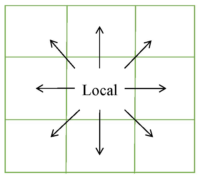
2.1. Spatial Weight Matrix

The spatial weight matrix is an indispensable element in the spatial econometric model. The spatial weight matrix can incorporate the unique spatial relationships of variables into the econometric model. Common spatial weight matrices are first-order contiguity matrix, geographical distance matrix and economic distance matrix.

2.1.1. First-Order Contiguity Matrix

First order adjacency matrix is a type of adjacency matrix, which mainly reflects the relationship between the local area and surrounding areas, that is, there is a common vertex or boundary between the two regions (Figure 2). The matrix limits the effective range of spillover effect and emphasizes that only the queen contiguity regions have obvious spillover effect. For example, the effective range of knowledge spillover effect is within 300 km (generally beyond the scope of a province in China) [39]. The expression of the first-order adjacency matrix is as follows:

$${\mathrm{W}}_{\mathrm{ij}}^{\mathrm{C}}=\{\begin{array}{l}1, \mathrm{i} \mathrm{and} \mathrm{j} \mathrm{are} \mathrm{queen} \mathrm{contiguity} \mathrm{relations}\\ 0, \mathrm{others}\end{array}$$

(1)

2.1.2. Geographical Distance Matrix

Tobler’s First Law of Geography pointed out “Everything is related to everything else, but near things are more related to each other” [40]. The geographic distance matrix best reflects this idea. Although this matrix does not limit the scope of spillover effects, it is believed that spillover effects weakens with increasing geographic distance. The expression of geographical distance matrix is as follows:

$${\mathrm{W}}_{\mathrm{ij}}^{\mathrm{D}}=\{\begin{array}{c}1/{\mathrm{d}}^2, \mathrm{i}\ne \mathrm{j}\\ 0, \mathrm{i}=\mathrm{j}\end{array}$$

(2)

2.1.3. Another Matrix

With the popularity of spatial econometric method, adjacency matrix and geographical distance matrix have been unable to meet the needs of economic research, and more and more new spatial weight matrices have appeared. For example, technological distance matrix reflects the impact of technological consistency between regions on spillover effects [41], institutional distance matrix reflects the impact of institutional disparity on spillover effects [42], and economic distance reflects the impact of economic disparity on spillover effects [43], etc. Among them, the economic distance matrix is used most frequently.

2.2. Moran’s I Test

Spatial econometric models require that there must be significant spatial autocorrelation of the explained variables. A commonly used test is the Moran’s I Test, specifically, the global Moran’s I test and the local Moran’s I test.

2.2.1. Global Moran’s I Test

The global spatial autocorrelation test tests the spatial autocorrelation degree of the whole sample, which reflects the spatial dependence of attribute values. Global Moran’s I test is the most commonly used method, which can visualize the spatial aggregation characteristics of attribute values [44]. Formula (3) shows the calculation process of global Moran’s I value.

$${\mathrm{I}}_{\mathrm{t}}^{\mathrm{G}}=\raisebox{1ex}{${\sum }_{\mathrm{i}=1}^{\mathrm{n}}{\sum }_{\mathrm{j}=1}^{\mathrm{n}}{\mathrm{W}}_{\mathrm{ij}}\left({\mathrm{X}}_{\mathrm{i},\mathrm{t}}-\overline{{\mathrm{X}}_{\mathrm{t}}}\right)\left({\mathrm{X}}_{\mathrm{j},\mathrm{t}}-\overline{{\mathrm{X}}_{\mathrm{t}}}\right)$}\!\left/ \!\raisebox{-1ex}{${\mathrm{S}}^2{\sum }_{\mathrm{i}=1}^{\mathrm{n}}{\sum }_{\mathrm{j}=1}^{\mathrm{n}}{\mathrm{W}}_{\mathrm{ij}}$}\right.$$

(3)

where i and j are individual labels; n is the number of samples; t is the time; ${\mathrm{X}}_{\mathrm{i}}$, ${\mathrm{X}}_{\mathrm{j}}$ and $\overline{\mathrm{X}}$ are the attribute value of i, j and average; ${\mathrm{W}}_{\mathrm{ij}}$ is the spatial weight matrix; ${\mathrm{S}}^2$ is the variance of the attribute value. The value of Moran’s I $\in \left[-1, 1\right]$. When $0<{\mathrm{I}}^{\mathrm{G}}<1$, there is a positive spatial agglomeration; when ${\mathrm{I}}^{\mathrm{G}}=0$, there is no spatial agglomeration, which means the attribute value is randomly distributed; when $-1<{\mathrm{I}}^{\mathrm{G}}<0$, there is a negative spatial agglomeration.

2.2.2. Local Moran’s I Test

Global spatial autocorrelation test can only test whether there is spatial autocorrelation in the whole sample, but it cannot judge the spatial autocorrelation characteristics of attribute values. We need to use the local spatial autocorrelation test to further explore the spatial autocorrelation characteristics of each attribute value (high-high agglomeration, low-low agglomeration, high-low agglomeration and low-high agglomeration). Moran scatter plot is one of the methods commonly used to test the characteristics of local regional aggregation. Formula (4) shows its calculation process.

$${\mathrm{I}}_{\mathrm{i}, \mathrm{t}}^{\mathrm{L}}=\raisebox{1ex}{$\left({\mathrm{X}}_{\mathrm{i},\mathrm{t}}-\overline{{\mathrm{X}}_{\mathrm{t}}}\right){\sum }_{\mathrm{j}=1}^{\mathrm{n}}{\mathrm{W}}_{\mathrm{ij}}\left({\mathrm{X}}_{\mathrm{j},\mathrm{t}}-\overline{{\mathrm{X}}_{\mathrm{t}}}\right)$}\!\left/ \!\raisebox{-1ex}{${\mathrm{S}}^2$}\right.$$

(4)

The meaning of each symbol is the same as above. In addition, when ${\mathrm{I}}^{\mathrm{L}}>0$, there is H-H or L-L agglomeration characteristics in adjacent areas; when ${\mathrm{I}}^{\mathrm{L}}<0$, there is L-H or H-L agglomeration characteristics in adjacent areas; when ${\mathrm{I}}^{\mathrm{L}}=0$, there is no local agglomeration characteristics in adjacent areas.

2.3. Description of Spatial Econometric Model

Common spatial econometric models include spatial lag model (SLM), spatial error model (SEM), and spatial Durbin model (SDM). SLM refers to the spatial lag of the explained variable, rather than the traditional time lag. The combination of the spatial lag and the explained variable is used as an explanatory variable to reflect the influence of the explained variable in other regions in the whole on the local. SEM can deal with spatial spillover effects caused by missing important variables or unobservable random shocks, that is, assuming that the disturbance term has spatial dependence. The characteristic of SDM is to add a combination of explanatory variables and spatial lags as new explanatory variables to reflect the influence of explanatory variables in other regions in the whole on the local. Formulas (5)–(7) are the general forms of SLM, SEM and SDM, respectively:

$$\mathrm{Y}=\mathsf{\alpha }\mathrm{WY}+\mathsf{\beta }\mathrm{X}+\mathsf{\epsilon }$$

(5)

$$\mathrm{Y}=\mathsf{\alpha }\mathrm{WY}+\mathsf{\beta }\mathrm{X}+\mathsf{\delta }\mathrm{WX}+\mathsf{\epsilon }$$

(6)

$$\begin{array}{c}\mathrm{Y}=\mathsf{\beta }\mathrm{X}+\mathsf{\mu }\\ \mathsf{\mu }=\mathrm{M}\mathsf{\mu }+\mathsf{\epsilon }\end{array}$$

(7)

where $\mathrm{W}$ and $\mathrm{M}$ are spatial weight matrices; $\mathsf{\alpha }$, $\mathsf{\beta }$ and $\mathsf{\delta }$ are coefficients of corresponding variables, and $\mathsf{\epsilon }$ is a random error term.

2.4. Entropy Method

Too many variables will likely lead to multicollinearity problems, and in this study, we will develop a multidimensional, innovation agglomeration-based indicator system that can facilitate land use transition. The entropy method is an effective method for evaluating comprehensive indicators. It can effectively reduce the dimensionality of indicators and give higher weights to secondary indicators with greater entropy (degree of variation), thus obtaining an efficient composite indicator. A brief calculation of the entropy method is as follows:

Step 1. A standardised matrix of indicator evaluation systems (${\mathrm{c}’}_{\mathrm{ab},\mathrm{t}}$) is created. where $\mathrm{a}$ is the cross-sectional individual $\mathrm{a}$ ($1\le \mathrm{a}\le \mathrm{n}$); b is the indicator b ($1\le \mathrm{b}\le \mathrm{k}$), and t is the period t.

$${\mathrm{c}’}_{\mathrm{ab},\mathrm{t}}=\raisebox{1ex}{${\mathrm{c}}_{\mathrm{ab},\mathrm{t}}-\underset{\mathrm{k}}{\min }\left|{\mathrm{c}}_{\mathrm{ab},\mathrm{t}}\right|$}\!\left/ \!\raisebox{-1ex}{$\underset{\mathrm{k}}{\max }\left|{\mathrm{c}}_{\mathrm{ab},\mathrm{t}}\right|-\underset{\mathrm{k}}{\min }\left|{\mathrm{c}}_{\mathrm{ab},\mathrm{t}}\right|$}\right.$$

(8)

Step 2. Formula (9) is the calculation of the information entropy (${\mathrm{E}}_{\mathrm{b},\mathrm{t}}$) for the indicator b in period t, and Formula (10) is the calculation of the weight for the indicator b in period t (${\mathrm{weight}}_{\mathrm{b},\mathrm{t}}$).

$$\begin{array}{c}{\mathrm{E}}_{\mathrm{b},\mathrm{t}}=-\ln {\left(\mathrm{n}\right)}^{-1}{\displaystyle \sum _{\mathrm{a}=1}^{\mathrm{n}}}\left({\mathrm{P}’}_{\mathrm{ab},\mathrm{t}}\right)\ln \left({\mathrm{P}’}_{\mathrm{ab},\mathrm{t}}\right)\\ \mathrm{s}.\mathrm{t}.{ \mathrm{P}’}_{\mathrm{ab},\mathrm{t}}=\raisebox{1ex}{${\mathrm{c}’}_{\mathrm{ab},\mathrm{t}}$}\!\left/ \!\raisebox{-1ex}{${\sum }_{\mathrm{a}=1}^{\mathrm{n}}{ \mathrm{c}\prime }_{\mathrm{ab},\mathrm{t}}$}\right.\end{array}$$

(9)

$${\mathrm{weight}}_{\mathrm{b},\mathrm{t}}=\raisebox{1ex}{$1-{\mathrm{E}}_{\mathrm{b},\mathrm{t}}$}\!\left/ \!\raisebox{-1ex}{$\mathrm{b}-{\sum }^{ }{\mathrm{E}}_{\mathrm{b},\mathrm{t}}$}\right.$$

(10)

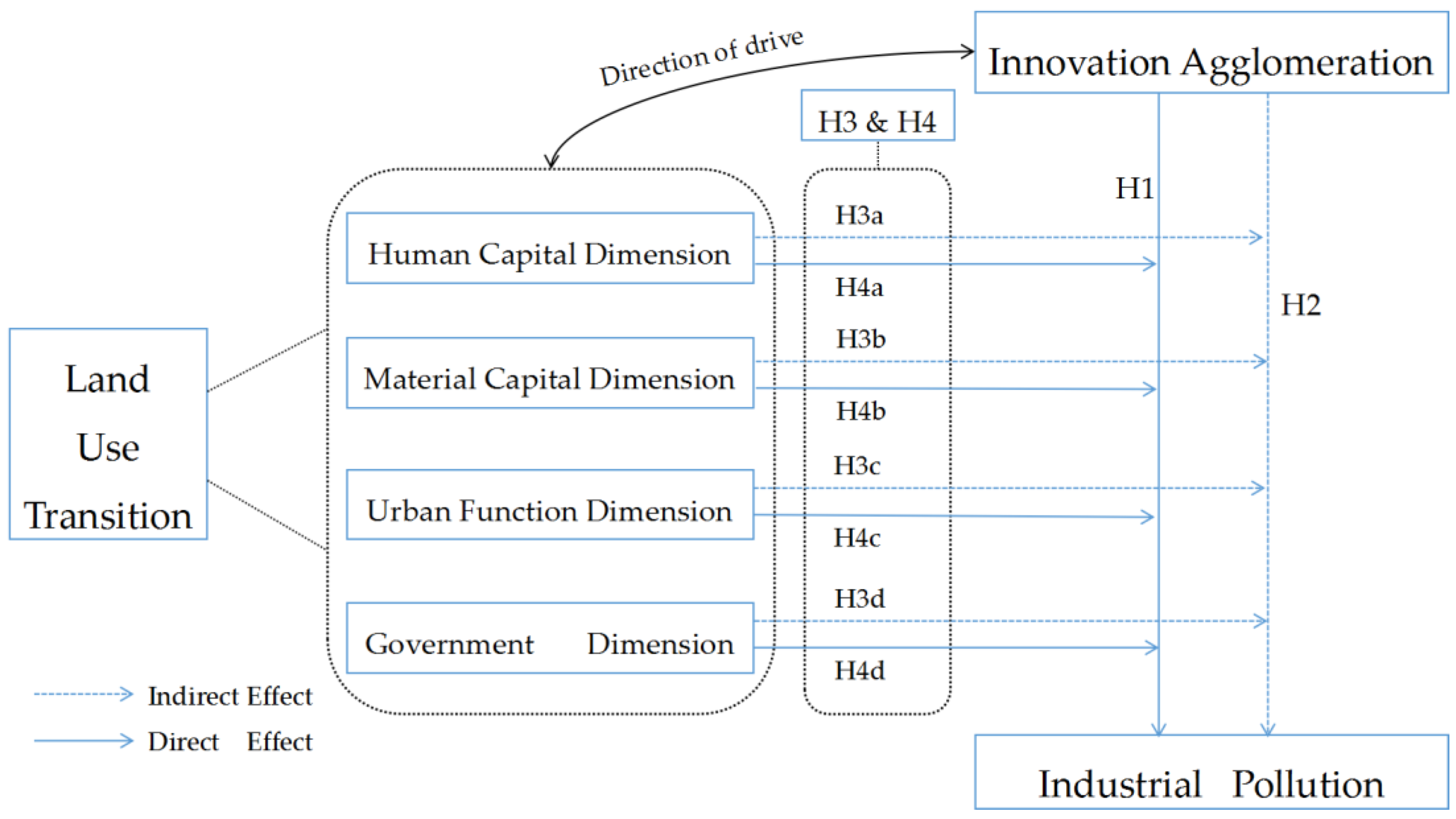
3. Design of Variables and Models

3.1. Explained Variable

Industrial pollution covers a wide range, but in this study, it refers specifically to “three wastes” (industrial effluent, industrial waste gas and industrial waste residue) pollution. Considering the availability of data, this study uses industrial effluent emissions, industrial SO₂ emissions and industrial soot emissions to measure the discharge of “three wastes”, respectively. Due to the different scales of regions, the absolute value data is easy to make the research conclusion “unfair”. Therefore, with reference to the design logic of location quotient, this study reduces the dimension of these 3 types of data into a kind of relative value data. The process is as follows:

Step 1. ${\mathrm{e}}_{\mathrm{it},\mathrm{p}}$ is the total emission of industrial pollution p (p = 3) of province i in period t; ${\mathrm{Y}}_{\mathrm{it}}$ is the actual total industrial output value of province i in period t, and ${\mathrm{E}}_{\mathrm{it},\mathrm{p}}$ is the economic efficiency of industrial pollution emission.

$${\mathrm{E}}_{\mathrm{it},\mathrm{p}}=\raisebox{1ex}{${\mathrm{e}}_{\mathrm{it},\mathrm{p}}$}\!\left/ \!\raisebox{-1ex}{${\mathrm{Y}}_{\mathrm{it}}$}\right.$$

(11)

Step 2. ${\mathrm{NE}}_{\mathrm{it},\mathrm{p}}$ is the economic efficiency of national industrial pollution emission in China. The 30 cross-section samples are represented by “30”.

$${\mathrm{NE}}_{\mathrm{it},\mathrm{p}}={\displaystyle \sum }_{\mathrm{i}=1}^{30}\raisebox{1ex}{${\mathrm{e}}_{\mathrm{it},\mathrm{p}}$}\!\left/ \!\raisebox{-1ex}{${\mathrm{Y}}_{\mathrm{it}}$}\right.$$

(12)

Step 3. Calculate the relative value of industrial pollution emission variables ($\mathrm{Ind}\_{\mathrm{pol}}_{\mathrm{it}}$). The higher the $\mathrm{Ind}\_{\mathrm{pol}}_{\mathrm{it}}$ is, the greater and the more serious the industrial pollution is; otherwise, the smaller the industrial pollution is, the lighter the industrial pollution is.

$$\mathrm{Ind}\_{\mathrm{pol}}_{\mathrm{it}}=\raisebox{1ex}{${\mathrm{E}}_{\mathrm{it},\mathrm{p}}$}\!\left/ \!\raisebox{-1ex}{${\mathrm{NE}}_{\mathrm{it},\mathrm{p}}$}\right.$$

(13)

3.2. Explanatory Variables

This study uses innovation agglomeration to represent the background of innovation-driven, so the moderate variable is innovation agglomeration (Inno_agg). The core explanatory variables reflect land use transition in the direction of innovation agglomeration and contain human capital dimension, material capital dimension, urban function dimension and government dimension. In addition, we have further set further Hypotheses H3 and H4 in this section.

3.2.1. Innovation Agglomeration

According to the above, innovation agglomeration emphasizes the concentration of innovation level in a region. Due to the type of available data and in order to reduce the potential for multicollinearity, this study uses the number of granted patents, which is processed to remove the effect of economic volume, to reflect more realistically the level of innovation agglomeration in the region. The processing steps are as follows:

$$\mathrm{Inno}\_{ \mathrm{agg}}_{\mathrm{it},\mathrm{p}}={\displaystyle \sum }_{\mathrm{i}=1}^{30}\raisebox{1ex}{${\mathrm{e}}_{\mathrm{it},\mathrm{p}}$}\!\left/ \!\raisebox{-1ex}{${\mathrm{G}}_{\mathrm{it}}$}\right.$$

(14)

where, $\mathrm{Inno}\_{ \mathrm{agg}}_{\mathrm{it},\mathrm{p}}$ represents level of innovation agglomeration of province i in period t. ${\mathrm{G}}_{\mathrm{it}}$ is GDP of province i in period t.

3.2.2. Human Capital Dimension

Knowledge is the original force of innovation-driven, and people are the carrier and core of knowledge. On the one hand, the higher the human capital of a region, the higher the innovation development of the region, the higher the rate of return on capital, thereby promoting land use transition and achieving energy conservation and emission reduction. On the other hand, higher levels of human capital will require a higher quality of life. These will force the local government to improve their infrastructure and beautify the environment to retain talents and elites. Accordingly, this study selects the following three variables to reflect the level of human capital and makes further hypotheses. (I) Population density. People are agglomerated and will gather in areas with more employment opportunities, a more developed economy and a higher living environment. Observing domestic and foreign cities, it can be found that the population density of such high-quality cities is usually high (of course, it does not mean that cities with higher population density must be high-quality). (II) Average educational level. Education is a medium for passing on knowledge and the basis for generating new knowledge. Innovative agglomeration will attract more highly educated people to settle here, which will increase the average education level of local residents [45]. Average educational level is proportion of (population of college and above * 16 + population of high school * 12 + population of junior high school * 9+population of elementary school * 6) in population over 6 years old. (III) Full-time equivalent of R & D personnel. It reflects the degree of hard work of scientific researchers in the region. R & D is a time-consuming and labour-intensive process, and a large number of valuable innovations are based on the work of scientific researchers day and night. The average weights corresponding to urban population density, average educational level and full-time equivalent of R & D personnel are 0.2907, 0.2280 and 0.48124, respectively (Appendix A

Table A1. Weight of human capital dimension.

Year	Urban Population Density	Average Educational Level	Full-Time Equivalent of R & D Personnel	Year	Urban Population Density	Average Educational Level	Full-Time Equivalent of R & D Personnel
2018	0.311	0.295	0.394	2011	0.183	0.169	0.647
2017	0.285	0.288	0.428	2010	0.307	0.197	0.496
2016	0.175	0.160	0.665	2009	0.326	0.204	0.470
2015	0.458	0.222	0.320	2008	0.338	0.293	0.369
2014	0.364	0.219	0.417	2007	0.228	0.213	0.559
2013	0.177	0.152	0.670	2006	0.240	0.245	0.515
2012	0.389	0.307	0.304

for the complete data).

Hypothesis 3a (H3a).

The land use transition driven by human capital dimension can reduce industrial pollution emissions on the region.

Hypothesis 4a (H4a).

The land use transition driven by human capital dimension can reduce industrial pollution emissions on surrounding regions.

3.2.3. Material Capital Dimension

Just as production and operation are inseparable from material capital investment, innovation requires a lot of capital support (such as the development of COVID-19 vaccines). In terms of innovation agglomeration, it will gather a large amount of material capital (mainly capital). On the one hand, money capital has a certain degree of speculation. Therefore, high capital clusters often have a higher rate of return on capital, thereby accelerating land use transition. On the other hand, the agglomeration of material capital cannot only speed up the progress of scientific research but also clear its funding barriers, thereby improving various pollution emission, also alleviating the problem of “financing difficulties” for companies using environmental protection equipment. Accordingly, this study chooses the following three variables to reflect level of material capital and makes further hypotheses. (I) Internal expenditure of R & D funds. It refers to the actual expenditure of enterprises and institutions for internal R & D activities (including basic research, applied research and experimental development). This is the most intuitive capital investment directly used for scientific research. (II) Financial institutions density. Financial institutions can promote the financing, which is the inevitable outcome of financial development to a certain period. High financial institutions density is the inevitable product of innovation development. It can not only improve the investment and financing efficiency of enterprises but also form a competitive environment, thus reducing the investment and financing costs [46]. The average weights corresponding to internal expenditure of R & D funds and financial institutions density are 0.6072 and 0.3928, respectively (Appendix A

Table A2. Weight of material capital dimension.

Year	Internal Expenditure of R & D Funds	Financial Institutions Density	Year	Internal Expenditure of R & D Funds	Financial Institutions Density
2018	0.561	0.439	2011	0.644	0.356
2017	0.610	0.390	2010	0.531	0.469
2016	0.696	0.304	2009	0.695	0.305
2015	0.580	0.420	2008	0.770	0.230
2014	0.451	0.549	2007	0.508	0.492
2013	0.629	0.371	2006	0.595	0.405
2012	0.624	0.376

for the complete data).

Hypothesis 3b (H3b).

The land use transition driven by material capital dimension can reduce industrial pollution emissions on the region.

Hypothesis 4b (H4b).

The land use transition driven by material capital dimension can reduce industrial pollution emissions on surrounding regions.

3.2.4. Urban Function Dimension

Urban function refers to the role and division of labour that a city plays in the economic and social development of a certain area, and it can also be simply described as the characteristics of a city. Urban development often has a significant negative impact on ecosystems [47], especially in developing countries that need to develop industries to improve their economic levels. After the reform and opening-up, the industrial-based development mode has brought “miracle growth” to China, but it has also been accompanied by many environmental problems. At that time, developing industry and increasing GDP were the main theme of most cities. Nowadays, with China’s national power is becoming stronger and stronger, people’s requirements for the quality of the living environment are constantly increasing, and China’s economic development has new requirements, that is, an innovation-driven development mode. In the process of innovation agglomeration, the urban functions need to be improved, and land use transition gradually is taking shape. On the one hand, the industrial structure of the city has changed, and the proportion of the secondary industry has decreased, while the proportion of the tertiary industry has increased year by year, which reduces the industrial pollution emissions. On the one hand, the industrial structure of cities has undergone changes, the proportion of the secondary industry has decreased, and the proportion of the tertiary industry has increased year by year, reducing industrial pollution emissions. On the other hand, as the government’s focus gradually shifts to the quality of life of residents, the city’s infrastructure will be improved accordingly. In the context of innovation agglomeration, local governments will build more humane and better infrastructure to meet the development needs of innovation, thereby accelerating land use transition and reducing industrial pollution emissions. Accordingly, this study chooses the following two variables to reflect level of urban function and makes further hypotheses. (I) Industrial structure evolution. Kuznets defines the industrial structure evolution as a re-allocation process of economic resources among agriculture, industry and service industries [48,49]. With the increase in economic development and the level of innovation agglomeration, the trend of economic servitization has accelerated, and the proportion of tertiary industry in GDP has also increased, thereby reducing the level of industrial pollution emissions. Although the industrial structure evolution is a comprehensive process, this study mainly focuses on the change phenomenon of the primary, secondary, and tertiary industries. Therefore, the ratio of tertiary industry’s GDP to total GDP is used to measure it. (II) Urban road area per capita. With the deepening of urbanization and the adjustment of urban functions, infrastructure is developing in the direction of convenience. Urban road area per capita directly reflects the city’s traffic convenience and indirectly reflects the city’s tendency to improve the life quality of residents. The average weights corresponding to industrial structure evolution and urban road area per capita are 0.6961 and 0.30392, respectively (Appendix A

Table A3. Weight of urban function dimension.

Year	Industrial Structure Evolution	Urban Road Area Per Capita	Year	Industrial Structure Evolution	Urban Road Area Per Capita
2018	0.680	0.320	2011	0.725	0.275
2017	0.715	0.285	2010	0.641	0.359
2016	0.737	0.263	2009	0.615	0.385
2015	0.771	0.229	2008	0.669	0.331
2014	0.800	0.200	2007	0.639	0.361
2013	0.777	0.223	2006	0.533	0.467
2012	0.748	0.252

for the complete data).

Hypothesis 3c (H3c).

The land use transition driven by urban function dimension can reduce industrial pollution emissions on the region.

Hypothesis 4c (H4c).

The land use transition driven by urban function dimension can reduce industrial pollution emissions on surrounding regions.

3.2.5. Government Dimension

The government dimension reflects what the government has done to strengthen the role of innovation agglomeration in industrial pollution reduction. China’s special national conditions and development history determine that the position and authority of the Communist Party of China as the ruling party are recognized [50], and the behaviour of local governments has a strong influence on social development [10]. On the one hand, innovation agglomeration urges the government to further increase the investment in science and technology expenditure in the general government budget, promote innovation and development, so as to promote land use transition and reduce industrial pollution emissions. On the other hand, under the requirement of sustainable development, the local government has restricted the pollution emission of enterprises with large industrial pollution emission, and gradually controlled the total industrial pollution emission from the total amount. Accordingly, this study chooses the following two variables to reflect the government dimension and makes further hypotheses. (I) Proportion of technology expenditure. Similar to internal expenditure of R & D funds, this variable is the proportion of science and technology expenditure in the general government budget, which reflects the government’s support and attitude to science and technology research. (II) Green coverage. Since it is difficult to directly measure the degree of government restrictions on industrial pollution emissions from enterprises, this study uses green coverage to indirectly reflect the government’s focus on the environment. The average weights corresponding to proportion of technology expenditure and green coverage are 0.7636 and 0.2364, respectively (Appendix A

Table A4. Weight of government dimension.

Year	Proportion of Technology Expenditure	Green Coverage	Year	Proportion of Technology Expenditure	Green Coverage
2018	0.793	0.207	2011	0.767	0.233
2017	0.755	0.245	2010	0.865	0.135
2016	0.677	0.323	2009	0.743	0.257
2015	0.792	0.208	2008	0.660	0.340
2014	0.849	0.151	2007	0.854	0.146
2013	0.673	0.327	2006	0.750	0.250
2012	0.751	0.249

for the complete data).

Hypothesis 3d (H3d).

The land use transition driven by government dimension can reduce industrial pollution emissions on the region.

Hypothesis 4d (H4d).

The land use transition driven by government dimension can reduce industrial pollution emissions on surrounding regions.

3.3. Control Variables

There are many factors that affect industrial pollution. The core explanatory variable of this article is only to filter out variables that can promote land use transition from the perspective of innovation agglomeration. Therefore, control variables should also be selected from the following aspects to prevent endogenous problems caused by omission of important explanatory variables. (I) Per capita GDP (Per_GDP). Buryn et al. found a close relationship between economic development and pollution emissions [51]. On the one hand, the higher the per capita GDP of a region, the higher the residents’ requirements for the quality of life and living environment. On the other hand, companies that can support a high level of per capita GDP often have a higher rate of return on investment, which is difficult for traditional industrial companies to achieve. (II) Foreign direct investment (FDI). In the early period of reform and opening-up, China had cheap labour, raw materials and land, which was extremely attractive to foreign manufacturers. They can use cheap production factors and perform corporate social responsibilities with low standards. However, with the increase in the cost of setting up manufactures in China and the Chinese awareness of environmental protection, the role of FDI in increasing industrial pollution emissions may weaken or even reverse [52]. This is not the focus of this article. However, it is undeniable that FDI in this study is a good control variable reflecting foreign influence. (III) Energy structure. Wang et al. found that there is a highly positive correlation between the proportion of coal energy and industrial pollution [53]. When the proportion of traditional coal energy drops, it indicates that the proportion of other relatively clean energy (wind power, hydroelectric power, etc.) in China has risen, thereby affecting industrial pollution emissions. Accordingly, this study uses the ratio of total electricity generation to total energy consumption to measure the energy structure. In addition, the converted standard coal coefficient (1.229 tonnes of standard coal/10,000 kWh) is used to convert the units of electricity generation into million tonnes of standard coal.

Table 1. Variable description.

Type	Variable	Unit	Obs	Mean	Std.	Label
Explained variable	Industrial pollution	-	390	4.4162	0.7752	Ind_pol
Moderate variable	Innovation agglomeration	item	390	9.0124	1.5499	Inno_agg
Explanatory variables (Human capital dimension)	Urban population density	person/km2	390	7.8374	0.4484	Human
	Average educational level	year/person	390	2.1703	0.1067
	Full-time equivalent of R & D personnel	10,000 man-year	390	10.9526	1.1148
Explanatory variables (Material capital dimension)	Internal expenditure of R & D funds	10,000 yuan	390	14.1989	1.4054	Material
	Financial institutions density	Unit/km2	390	−5.6902	0.4764
Explanatory variables (Urban function dimension)	Industrial Structure Evolution	%	390	3.7468	0.1932	Urban
	Urban road area per capita	m2/person	390	2.5838	0.3305
Explanatory variables (Government dimension)	Proportion of technology expenditure	%	390	−1.0851	0.4764	Government
	Green coverage	%	390	3.6197	0.1338
Control variables	Per capita GDP	yuan/person	390	10.4694	0.5826	Per_GDP
	Foreign direct investment	10,000 dollar	390	12.5964	1.6338	FDI
	Energy structure	%	390	2.6562	0.4717	Ener_stru

Mean and Std. are both values in logarithmic form.

summarizes the indicator system.

3.4. Data Resource

Since 2006 (the starting point of the 11th Five-Year Plan), China has strictly controlled pollution emissions and strengthened its efforts to carry out green development. Therefore, this study uses the panel data of 30 provinces in China after 2006 (2006–2018) for research. In view of the integrity and availability of the data, the Tibet Autonomous, Hong Kong, Macao and Taiwan were excluded. All raw data comes from China Statistical Yearbook, China statistical yearbook on Science and technology, provincial statistical yearbook. Some of the missing data are supplemented using the moving average method.

3.5. Model Design

This study takes the form of the Cobb-Douglas production function and considers industrial pollution emissions as an “output”. By taking the logarithm of both sides of the C-D production function, we transform the equation into a linear function and at the same time mitigate the heteroskedasticity generated by the panel data. ${\mathsf{\epsilon }}_{\mathrm{it}}$ is the random perturbation term.

$$\ln {\mathrm{Y}}_{\mathrm{it}}={\mathsf{\theta }}_{\mathrm{it}}+\mathsf{\beta }\ln {\mathrm{X}}_{\mathrm{it}}+\mathsf{\gamma }\ln {\mathrm{Control}}_{\mathrm{it}}+{\mathsf{\epsilon }}_{\mathrm{it}}$$

(15)

Since the spatial Durbin model has the widest range of applicability, we transform Formula (15) into the form of SDM.

$$\ln {\mathrm{Y}}_{\mathrm{it}}=\mathsf{\beta }\ln {\mathrm{X}}_{\mathrm{it}}+{\mathsf{\delta }}_1\mathrm{W}\ln {\mathrm{X}}_{\mathrm{it}}+\mathsf{\gamma }\ln {\mathrm{Control}}_{\mathrm{it}}+{\mathsf{\delta }}_2\mathrm{W}\ln {\mathrm{Control}}_{\mathrm{it}}+{\mathsf{\epsilon }}_{\mathrm{it}}$$

(16)

Panel models usually use either fixed effects or random effects. Random effects assume that all regression variables containing individual random effects are exogenous and are often used to “see the big picture”. Fixed effects, on the other hand, assume that the variables containing the effects of individuals are endogenous. [53] Therefore, as the study is for 30 provinces in China, fixed effects are used in this paper. There are three forms of fixed effects in the spatial panel model: spatial fixed effect, time-period fixed effect and spatial and time-period (S&T) fixed effect. The spatial fixed effect reflects characteristics that do not vary with time but vary with individuals (${\mathsf{\sigma }}_{\mathrm{i}}$), while the time-period fixed effect reflects characteristics that do not vary with individuals but vary with time (${\mathsf{\tau }}_{\mathrm{t}}$). Since industrial pollution emissions have distinct regional characteristics and Yu et al. found that smog pollution has a time-varying trend and diffusivity [34], the S&T fixed effect model was used in this study and the spatial lag term of the explanatory variable (Ind_pol) was added to control for this (see Formula (17)).

$$\ln {\mathrm{Y}}_{\mathrm{it}}=\mathsf{\alpha }\mathrm{W}\ln {\mathrm{Y}}_{\mathrm{it}}+\mathsf{\beta }\ln {\mathrm{X}}_{\mathrm{it}}+\mathsf{\delta }\mathrm{W}\ln {\mathrm{X}}_{\mathrm{it}}+\mathsf{\gamma }\ln {\mathrm{Control}}_{\mathrm{it}}+\mathsf{\omega }\mathrm{W}\ln {\mathrm{Control}}_{\mathrm{it}}+{\mathsf{\sigma }}_{\mathrm{i}}+{\mathsf{\tau }}_{\mathrm{t}}+{\mathsf{\epsilon }}_{\mathrm{it}}$$

(17)

Finally, substituting the variables mentioned in the article into Formula (17), get Formula (18). In which, ${\mathrm{Explanatory}}_{\mathrm{v},\mathrm{it}}$ represents the explanatory variables for period t of province i in dimension v, that is, human capital dimension, material capital dimension, urban function dimension and government dimension.

$$\begin{array}{ll}\ln \mathrm{Ind}\_{ \mathrm{pol}}_{\mathrm{it}}=& \mathsf{\alpha }\mathrm{W}\ln \mathrm{Ind}\_{ \mathrm{pol}}_{\mathrm{it}}+{\mathsf{\beta }}_1\mathrm{W}\ln \mathrm{Inno}\_{ \mathrm{agg}}_{\mathrm{it}}\\ & +{\mathsf{\beta }}_2\ln \left({\mathrm{Explanatory}}_{\mathrm{v},\mathrm{it}}\ast \ln \mathrm{Inno}\_{ \mathrm{agg}}_{\mathrm{it}}\right)\\ & +{\mathsf{\delta }}_1\mathrm{W}\ln \mathrm{Inno}\_{ \mathrm{agg}}_{\mathrm{it}}\\ & +{\mathsf{\delta }}_2\mathrm{W}\ln \left({\mathrm{Explanatory}}_{\mathrm{v},\mathrm{it}}\ast \ln \mathrm{Inno}\_{ \mathrm{agg}}_{\mathrm{it}}\right)\\ & +{\mathsf{\gamma }}_1\ln \mathrm{Per}\_{ \mathrm{GDP}}_{\mathrm{it}}+{\mathsf{\gamma }}_2\ln {\mathrm{FDI}}_{\mathrm{it}}+{\mathsf{\gamma }}_3\ln \mathrm{Ener}\_{ \mathrm{stru}}_{\mathrm{it}}\\ & +{\mathsf{\omega }}_1\mathrm{W}\ln \mathrm{Per}\_{ \mathrm{GDP}}_{\mathrm{it}}+{\mathsf{\omega }}_2\mathrm{W}\ln {\mathrm{FDI}}_{\mathrm{it}}+{\mathsf{\omega }}_3\mathrm{W}\ln \mathrm{Ener}\_{ \mathrm{stru}}_{\mathrm{it}}\\ & +{\mathsf{\sigma }}_{\mathrm{i}}+{\mathsf{\tau }}_{\mathrm{t}}+{\mathsf{\epsilon }}_{\mathrm{it}}\end{array}$$

(18)

4. Results

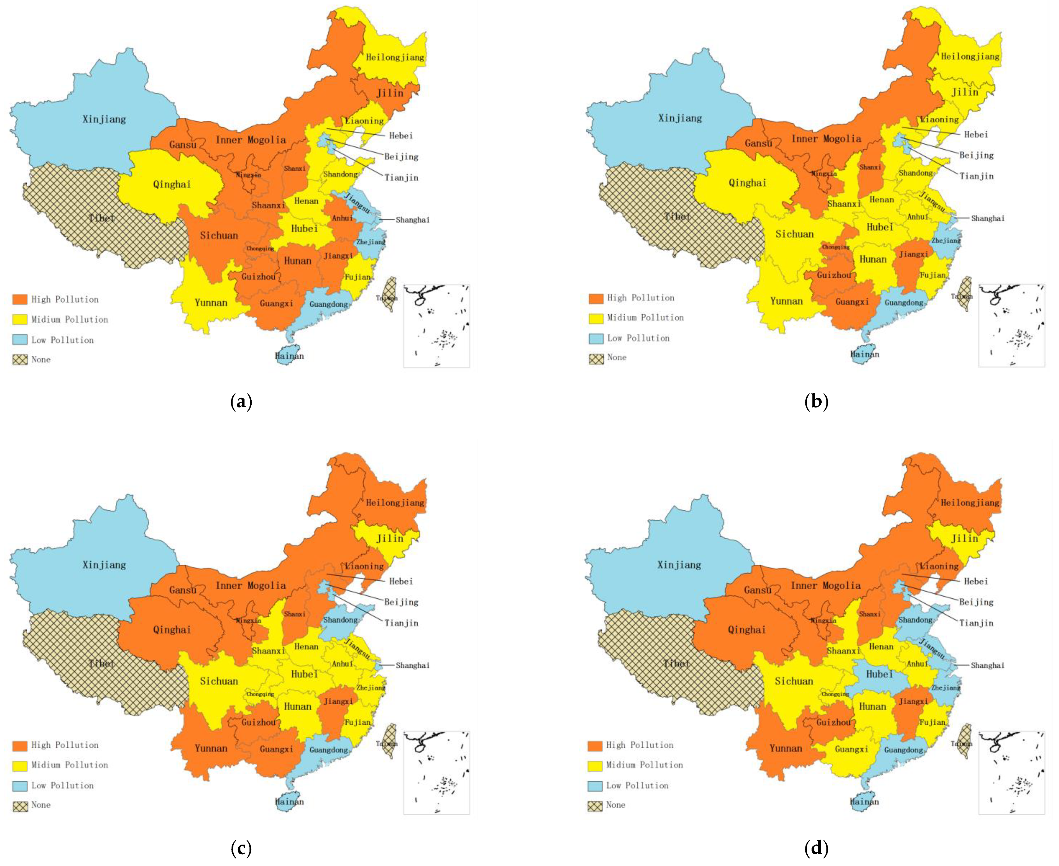
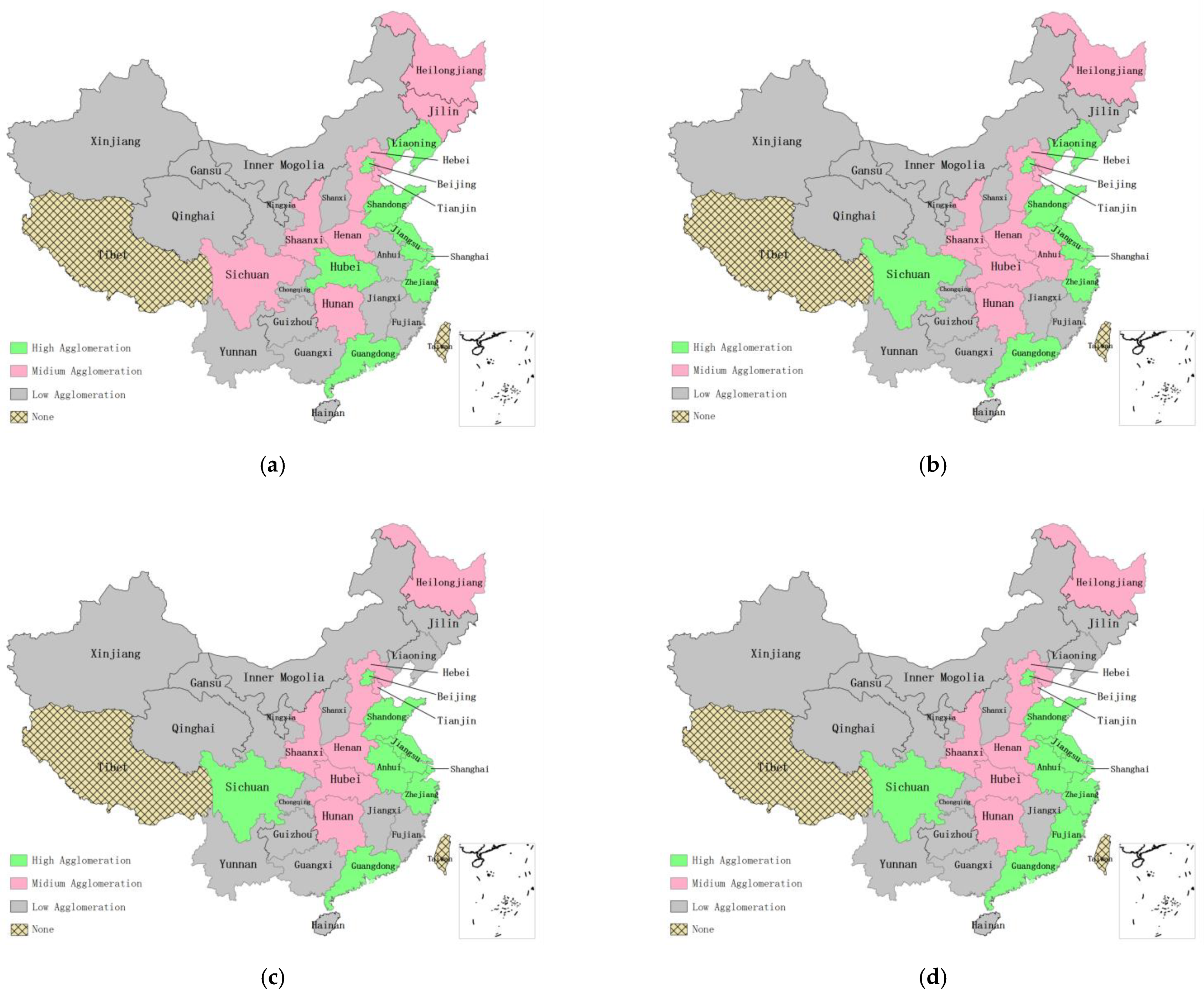
4.1. Analysis of Spatial-Temporal Evolution

4.1.1. Industrial Pollution

Figure 3 shows that the regions of medium and low industrial pollution are mostly the more economically developed regions, and there is a clear distribution characteristic—the eastern coastal region have less industrial pollution, while some parts of central and western China have more. However, over time, the eastern region solidified its low industrial pollution levels, while the central region generally maintained medium industrial pollution levels and northern China clearly behaved in a high industrial pollution trend.

4.1.2. Innovation Agglomeration

Figure 4 shows that, Overall, innovation agglomeration is more extreme across China’s provinces—there are fewer regions of high agglomeration and more regions of medium and low agglomeration. Analysing the spatial distribution pattern, it is clear that innovation agglomeration is high in the eastern region and low in the western region, with Sichuan Province standing out as the core province in western China. Combined with the time evolution pattern, it can be found that the divisional pattern has not changed significantly during the 13 years, indicating that the spatial distribution pattern has further solidified and behaved with obvious high and high agglomeration characteristics.

4.2. Spatial Regression Results

Table 2. Regression results.

Explanatory Variables	I	II	III	IV	V
Inno_agg	−0.2315 **	−0.3096 **	−0.2340 *	−0.2214 *	−0.2193 *
Human	0.0655 ***	-	-	-	-
Material	−0.1296 **	-	-	-	-
Urban	0.0264	-	-	-	-
Government	0.0828 **	-	-	-	-
Inno_agg * Human	-	−0.0627 ***	-	-	-
Inno_agg * Material	-	-	−0.0152 *	-	-
Inno_agg * Urban	-	-	-	−0.0018 *	-
Inno_agg * Government	-	-	-	-	−0.0104 *
Per_GDP	−0.4558 *	−0.4325 *	−0.4865 *	−0.4871 *	−0.4903 *
FDI	−0.1439 *	−0.1374 *	−0.1341 *	−0.1329 *	−0.1309 *
Ener_stru	−0.3496 *	−0.3658 *	−0.3709 *	−0.3784 *	−0.3693 *
W * Inno_agg	0.2287	0.1623	0.1853	0.2215	0.2171
W * Human	0.0424	-	-	-	-
W * Material	0.0076	-	-	-	-
W * Urban	0.0248	-	-	-	-
W * Government	−0.0382	-	-	-	-
W * Inno_agg * Human	-	−0.0403	-	-	-
W * Inno_agg * Material	-	-	−0.0390	-	-
W * Inno_agg * Urban	-	-	-	0.0185	-
W * Inno_agg * Government	-	-	-	-	−0.0145
W * Per_GDP	−0.6703 **	−0.7312 **	−0.7095 **	−0.7450 **	−0.7369 *
W * FDI	0.1292	0.1382	0.1372	0.1531	0.1467
W * Ener_stru	−0.8653 **	−0.8275 **	−0.8191 **	−0.8171 **	−0.8204 **
R-square	0.2320	0.2611	0.2625	0.2509	0.2594
Log-L	53.6512	48.3867	45.2893	44.0831	44.2472
rho	−2.51 **	−2,24 **	−2.35 **	−2.25 **	−2.32 **

***, **, and * respectively indicate statistical significance at the 1%, 5%, and 10% levels.

presents the regression results for the direct and indirect effects of the five regression in this study. Model I test Hypotheses H1 and H2. Models II, III, IV, and IV test hypotheses H3 and H4.

From Model I, the direct effect coefficient of innovation agglomeration is −0.2315 (significant), while its indirect effect coefficient is 0.2287 (insignificant). Therefore, hypothesis H1 holds, but Hypotheses H2 does not, i.e., innovation agglomeration helps to reduce industrial pollution emissions on the region, but it does not have a spillover effect.

In Models II–V, Hypotheses H3 and H4 can be tested by the direct and indirect effect coefficients of the interaction terms of innovation agglomeration and the explanatory variables (Human, Material, Urban and Government). The direct effect coefficients of the four models are −0.0627, −0.0152, −0.0018 and −0.0104, respectively, and all of them pass the 10% significance level test, indicating that Hypotheses H3 (H3a, H3b, H3c and H3d) holds, but the indirect effects are not significant, indicating that Hypotheses H4 (H4a, H4b, H4c and H4d) does not.

4.3. Robustness Tests

4.3.1. Spatial Autocorrelation Test

Spatial autocorrelation is the basis for spatial econometric model. Although industrial pollution is inherently spillover in nature, it is logical to use a spatial econometric model for the study. However, in order to be rigorous, this study still measured the spatial autocorrelation of industrial pollution between 2006 and 2018, and visualised the results using global Moran’s I statistics and Moran scatter.

Table 3. Global Moran’s I value.

Year	Moran’s I	p-Value	Year	Moran’s I	p-Value
2006	2.356	0.018	2013	1.192	0.117
2007	2.451	0.014	2014	1.762	0.078
2008	2.317	0.021	2015	1.690	0.091
2009	2.316	0.021	2016	1.794	0.073
2010	2.205	0.027	2017	1.624	0.096
2011	2.992	0.003	2018	1.523	0.128
2012	1.687	0.090

shows the global Moran’s I statistics in 2006–2018, which shows that the majority of p-values are less than 0.10, indicating that industrial pollution in China has spatial autocorrelation at the provincial level. Figure 5 shows that there are obvious agglomeration characteristics in the distribution of industrial pollution in China, among which, low-low agglomeration is predominant. In summary, it is reasonable to use spatial econometric models in this study.

4.3.2. Model Applicability Test

To test the superiority of SDM over SAR, we made the hypothesis that the spatial lag of the explanatory variables in the model, WX = 0. It was found that all regression models rejected the null hypothesis, i.e., SDM should be used for research rather than SAR.

To test the superiority of SDM over SEM, we made the hypothesis that the spatial lag of the explanatory variable in the model, WX = −rho * X. It was found that all regression models rejected the null hypothesis, i.e., SDM should be used for research rather than SEM.

In order to verify that the S&T fixed effect model outperforms the time-period fixed effect model and the spatial fixed effect model in this study, all regression models were tested using the F-test and the null hypothesis was rejected. (

Table 4. F statistic value.

	I	II	III	IV	V
Spatial fixed effect	115.86 ***	121.47 ***	120.71 ***	126.13 ***	119.75 ***
Time-period fixed effect	22.55 ***	36.54 ***	35.92 ***	37.86 ***	34.89 ***

*** indicate statistical significance at the 1% levels.

).

5. Discussions

Table 2 proves that Hypotheses H1 and H3 (H3a, H3b, H3c and H3d) are valid, while H2 and H4 (H4a, H4b, H4c and H4d) are not. This suggests that (1) innovation agglomeration contributes to the reduction of industrial emissions in the region but does not have a significant effect on its surrounding regions; (2) it is feasible to enhance the effect of innovation agglomeration on industrial pollution reduction by land use transition on the region, but this effect does not have a significant influence on the surrounding regions. Specifically: hypothesis H3a holds, which suggests that an increase in the human capital dimension will, on the one hand, help to drive land use transition and thus strengthen the reduction of industrial pollution emissions from innovation agglomeration; on the other hand, the government will be more active in implementing strategies to reduce emissions and retain elite talent. Based on the weight of the secondary indicators of human capital dimension, it can be further argued that full-time equivalent of R & D personnel plays the greatest role, followed by population density and finally average educational level. This enlightens us that increasing the workload of R & D personnel and attracting the inflow of foreign population can bring greater benefits. Hypothesis H3b holds, which suggests that an increase in the material capital dimension will help to remove financial barriers to research, ease the “difficulty of financing” the use of environmental equipment by firms, accelerate land use transition and reduce industrial pollution emissions. In addition, the demand of capitalists for adequate returns on capital will also increase the level of land use in the region, thus promoting land use change and reducing industrial pollution emissions. Based on the weight of the secondary indicator of material capital dimension, it can be further argued that although the role of internal expenditure of R & D funds in reducing emissions is stronger than that of financial institutions density, both are very important. This reveals to us that although R & D expenses are important, the role of financial institutions in financing should not be neglected, which reduces the difficulty of innovative enterprises in obtaining funds. Hypothesis H3c holds, indicating that the upgrading of the urban function dimension is conducive to the transition and upgrading of industries in the region, achieving land use transition while also reducing industrial pollution emissions and, on the other hand, encouraging the government to build more humane and innovative infrastructure, thus accelerating land use transition. Based on the weight of the secondary indicators of the urban function dimension, it can be further argued that industrial structure evolution is the main force in promoting innovation and achieving industrial pollution reduction, which reveals to us that promoting industrial structure upgrading and accelerating the service-oriented economy is a triple-win path of accelerating land use transition, promoting innovation and achieving environmental protection. Hypothesis H3d holds that the government’s efforts help to accelerate land use transition and reduce industrial pollution emissions. Based on the weights of the secondary indicators of the government dimension, it can be further argued that, on the one hand, the government, by supporting innovation development, has the guidance to promote land use transition and strengthen innovation agglomeration, thus reducing industrial pollution; on the other hand, the government’s greening efforts help retain elites and provide an environmental basis for innovation agglomeration, which also indirectly curbs industrial pollution emissions.

For other variables, the direct effect coefficient of Per_GDP is negative and passes the 10% significance level test. The indirect effect coefficient was also negative and passed the 10% significance level test. This indicates that an increase in per capita GDP within a region not only helps to reduce industrial pollution emissions in the region but also helps to reduce emissions in neighbouring regions. This is consistent with the findings of Buryn et al. [51]. The coefficient of the direct effect of FDI is negative and passes the 10% significance level test. However, its indirect effect is not significant. This suggests that as the Chinese and the government have become more environmentally conscious, the role of foreign investors in increasing emissions has been reversed and has instead helped to reduce industrial pollution, which is consistent with Jorgenson’s findings [52]. This is because China is focusing on bringing in high quality FDI (advanced production technologies) and gradually abandoning its role as a “processing plant”. The direct effect coefficient of energy structure is negative and passes the 10% significance level test. The indirect effect coefficient is also negative and passes the 10% significance level test. This indicates, when the proportion of traditional coal energy drops, that the proportion of other relatively clean energy (wind power, hydroelectric power, etc.) in China has risen, thereby affecting industrial pollution emissions. This is consistent with the results of Wang et al.’s study [53], implying the importance of energy structure transformation in reducing industrial pollution.

6. Conclusions

Innovation and environmental protection are the main themes of China’s development today, and the lack of efficient land use is one of the main problems of China’s development. This paper analyses the relationship between innovation agglomeration, land use transition and industrial pollution, and subtly investigates the question of whether innovation-oriented land use transition can reduce industrial pollution emissions. Using provincial-level data from 2006–2018, the paper draws conclusions through a spatial econometric model and proposes a series of targeted policy implications based on an analysis of the spatio-temporal evolution of industrial pollution and innovation agglomeration, in the hope of providing theoretical support for China’s triple-win development (innovation, land use transition and environmental protection).

The conclusions are as follows:

(1)

Both industrial pollution and innovation agglomeration have a clear spatial and temporal distribution. In eastern China, the level of industrial pollution is lower, while in northern China it is higher. Moreover, this distribution characteristic has become increasingly evident over time; innovation agglomeration is more extreme across China’s provinces—there are fewer regions of high agglomeration and more regions of medium and low agglomeration. Analysing the spatial distribution pattern, it is clear that innovation agglomeration is high in the eastern region and low in the western region. Moreover, this distribution characteristic has not changed significantly over time.

(2)

The land use transition towards an innovation-driven direction contributes to the reduction of industrial pollution emissions on the region but has no significant impact on the surrounding regions. In human capital dimension, full-time equivalent of R & D personnel plays the greatest role, followed by population density and finally average educational level; in material capital dimension, the role of internal expenditure of R & D funds is stronger than that of financial institutions density; in urban function dimension, the role of industrial structure evolution is significantly stronger than that of urban road area per capita, due to the high level of infrastructure development in China and the limited variation in urban road area per capita across regions; in government dimension, the role of proportion of technology expenditure is significantly stronger than that of green coverage for the same reasons as above.

(3)

In line with existing research, increasing per capita GDP and FDI and improving energy structure can help reduce industrial pollution. Moreover, increasing per capita GDP and improving energy structure can also generate positive spillover effects and promote the reduction of industrial pollution in neighbouring provinces.

Based on the above, we have obtained some inspiration on policy making:

(1)

Adhere to the policy of compulsory education, continue to strengthen the training of talents, improve the mechanism of training talents, and improve the treatment of talents, especially R & D personnel. For the eastern regions with a high degree of innovation agglomeration, various policies should be formulated for the introduction of talents to attract the inflow of more innovative talents.

(2)

Encourage and subsidise enterprises to undertake R & D; especially northern China, where the degree of innovation agglomeration is weak, should not be neglected because of its weak innovation agglomeration, but should instead be supported more vigorously, as these regions are heavily polluted by industry and their potential for improvement is enormous. Improve the distribution of financial institution outlets and ensure that a certain number of financial institutions are maintained throughout China to facilitate investment and financing for enterprises and to help them break down the barriers to financing.

(3)

Continue to improve supply-side reforms in order to promote the industrial structures. This is especially true for the more polluted regions of western and northern China. For the eastern regions, where pollution is low and the industrial structure is more advanced, there should be a targeted move towards demand-side reform. In addition, maintain or reduce the investment in road infrastructure, especially in the central and eastern regions, but infrastructure development in the western regions should be further strengthentened.

(4)

Strengthen financial support for science and technology research and development, and build a platform for cross-regional, cross-university and cross-disciplinary collaboration to increase the utilisation of research funds. At the same time, the government should continue to maintain the level of green coverage in all regions.

References

1. Dolk, H.; Vrijheid, M. The impact of environmental pollution on congenital anomalies. Br. Med. Bull. 2003, 68, 25–45. [Google Scholar] [CrossRef] [Green Version]
2. Grönqvist, H.; Nilsson, J.P.; Robling, P.-O. Understanding How Low Levels of Early Lead Exposure Affect Children’s Life Trajectories. J. Polit. Econ. 2020, 128, 3376–3433. [Google Scholar] [CrossRef]
3. Juan, B.; Ana, C.; Jean-Paul, V.; Omer, C.; Muriel, C. Protected areas in the Atlantic facing the hazards of micro-plastic pollution: First diagnosis of three islands in the Canary Current. Mar. Pollut. Bull. 2014, 80, 302–311. [Google Scholar]
4. Desforges, J.-P.W.; Galbraith, M.; Dangerfield, N.; Ross, P.S. Widespread distribution of microplastics in subsurface seawater in the NE Pacific Ocean. Mar. Pollut. Bull. 2014, 79, 94–99. [Google Scholar] [CrossRef]
5. Evangeliou, N.; Grythe, H.; Klimont, Z.; Heyes, C.; Eckhardt, S.; Lopez-Aparicio, S.; Stohl, A. Atmospheric transport is a major pathway of microplastics to remote regions. Nat. Commun. 2020, 11, 1–11. [Google Scholar] [CrossRef]
6. Olayinka, K.; Alo, B. Studies on Industrial Pollution in Nigeria: The effect of Textile effluents on the quality of Groundwater in some parts of Lagos. Niger. J. Health Biomed. Sci. 2004, 3, 44–50. [Google Scholar] [CrossRef]
7. Lloyd, O.L.; Smith, G.; Lloyd, M.M.; Holland, Y.; Gailey, F. Raised mortality from lung cancer and high sex ratios of births associated with industrial pollution. Occup. Environ. Med. 1985, 42, 475–480. [Google Scholar] [CrossRef]
8. Cameron, J.F. Radioisotope Techniques for Measurement and Control of Industrial Pollution. Meas. Control 1971, 4, 303–307. [Google Scholar] [CrossRef]
9. Ebiefung, A.A.; Udo, G. An industrial pollution emission control model. Comput. Ind. Eng. 1999, 37, 371–374. [Google Scholar] [CrossRef]
10. De Bruyn, S.; Bergh, J.V.D.; Opschoor, J. Economic growth and emissions: Reconsidering the empirical basis of environmental Kuznets curves. Ecol. Econ. 1998, 25, 161–175. [Google Scholar] [CrossRef]
11. Glaeser, E.L.; Kahn, M.E. The greenness of cities: Carbon dioxide emissions and urban development. J. Urban Econ. 2010, 67, 404–418. [Google Scholar] [CrossRef] [Green Version]
12. Cole, M.A. Trade, the pollution haven hypothesis and the environmental Kuznets curve: Examining the linkages. Ecol. Econ. 2004, 48, 71–81. [Google Scholar] [CrossRef]
13. Managi, S.; Hibiki, A.; Tsurumi, T. Does trade openness improve environmental quality? J. Environ. Econ. Manag. 2009, 58, 346–363. [Google Scholar] [CrossRef]
14. Ozturk, I.; Acaravci, A. The long-run and causal analysis of energy, growth, openness and financial development on carbon emissions in Turkey. Energy Econ. 2013, 36, 262–267. [Google Scholar] [CrossRef]
15. Su, Y.; Yu, Y.-Q. Spatial agglomeration of new energy industries on the performance of regional pollution control through spatial econometric analysis. Sci. Total Environ. 2020, 704, 135261. [Google Scholar] [CrossRef]
16. Zeng, D.Z.; Zhao, L. Pollution havens and industrial agglomeration. J. Environ. Econ. Manag. 2009, 58, 141–153. [Google Scholar] [CrossRef] [Green Version]
17. Han, L.; Kung, J.K.S. Fiscal incentives and policy choices of local governments: Evidence from China. J. Dev. Econ. 2015, 116, 89–104. [Google Scholar] [CrossRef]
18. Dean, J.M.; Lovely, M.E.; Wang, H. Are foreign investors attracted to weak environmental regulations? Evaluating the evidence from China. J. Dev. Econ. 2009, 90, 1–13. [Google Scholar] [CrossRef] [Green Version]
19. Zhu, C.; Lee, C.-C. The internal and external effects of air pollution on innovation in China. Environ. Sci. Pollut. Res. 2021, 28, 9462–9474. [Google Scholar] [CrossRef]
20. Ahn, S.J.; Yoon, H.Y. ‘Green chasm’ in clean-tech for air pollution: Patent evidence of a long innovation cycle and a technological level gap. J. Clean. Prod. 2020, 272, 122726. [Google Scholar] [CrossRef]
21. Omri, A.; Hadj, T.B. Foreign investment and air pollution: Do good governance and technological innovation matter? Environ. Res. 2020, 185, 109469. [Google Scholar] [CrossRef] [PubMed]
22. Ghosh, S. Examining carbon emissions economic growth nexus for India: A multivariate cointegration approach. Energy Policy 2010, 38, 3008–3014. [Google Scholar] [CrossRef]
23. Brunnermeier, S.B.; A Cohen, M. Determinants of environmental innovation in US manufacturing industries. J. Environ. Econ. Manag. 2003, 45, 278–293. [Google Scholar] [CrossRef]
24. Schumpeter, J.; Backhaus, U. The Theory of Economic Development; Springer: Boston, MA, USA, 2006; pp. 61–116. [Google Scholar]
25. Taylor, M.S.; Copeland, B.R. Trade, Growth and the Environment; NBER Working Paper; National Bureau of Economic Research: Cambridge, MA, USA, 2003; p. 9823. [Google Scholar]
26. Ji, X.; Wang, K.; Ji, T.; Zhang, Y.; Wang, K. Coupling Analysis of Urban Land Use Benefits: A Case Study of Xiamen City. Land 2020, 9, 155. [Google Scholar] [CrossRef]
27. Ji, Z.H.; Zhang, P. Spatial Difference and Driving Mechanism of Urban Land Use Efficiency Under the Environmental Constraints: Based on 285 Cities in China. China Land Sci. 2020, 34, 72–79. [Google Scholar] [CrossRef]
28. Huang, J.; Xue, D. Study on Temporal and Spatial Variation Characteristics and Influencing Factors of Land Use Efficiency in Xi’an, China. Sustainability 2019, 11, 6649. [Google Scholar] [CrossRef] [Green Version]
29. Yu, J.; Zhou, K.; Yang, S. Land use efficiency and influencing factors of urban agglomerations in China. Land Use Policy 2019, 88. [Google Scholar] [CrossRef]
30. Li, J.; Lewis, J.; Rowland, J.; Tappan, G.; Tieszen, L. Evaluation of land performance in Senegal using multi-temporal NDVI and rainfall series. J. Arid. Environ. 2004, 59, 463–480. [Google Scholar] [CrossRef]
31. Chen, C.-L. Establishing Urban Industrial Parks to Drive Regional Innovation System. Int. J. Autom. Smart Technol. 2012, 2, 283–286. [Google Scholar] [CrossRef]
32. Yun, W.; Zhu, D.; Tang, H. Reshaping and innovation of China land consolidation strategy. Trans. Chin. Soc. Agric. Eng. 2016, 32, 1–8. [Google Scholar]
33. Anselin, L. Spatial Effects in Econometric Practice in Environmental and Resource Economics. Am. J. Agric. Econ. 2001, 83, 705–710. [Google Scholar] [CrossRef]
34. Yu, X.; Shen, M.; Shen, W.; Zhang, X. Effects of Land Urbanization on Smog Pollution in China: Estimation of Spatial Autoregressive Panel Data Models. Land 2020, 9, 337. [Google Scholar] [CrossRef]
35. Romer, P.M. Increasing Returns and Long-Run Growth. J. Polit. Econ. 1986, 94, 1002–1037. [Google Scholar] [CrossRef] [Green Version]
36. Romer, P. Endogenous Technological Change. J. Polit. Econ. 1989, 98, 71–102. [Google Scholar] [CrossRef] [Green Version]
37. Motlagh, Z.K.; Lotfi, A.; Pourmanafi, S.; Ahmadizadeh, S.; Soffianian, A. Spatial modeling of land-use change in a rapidly urbanizing landscape in central Iran: Integration of remote sensing, CA-Markov, and landscape metrics. Environ. Monit. Assess. 2020, 192, 1–19. [Google Scholar] [CrossRef] [PubMed]
38. Tian, F.; Li, M.; Han, X.; Liu, H.; Mo, B. A Production–Living–Ecological Space Model for Land-Use Optimisation: A case study of the core Tumen River region in China. Ecol. Model. 2020, 437, 109310. [Google Scholar] [CrossRef]
39. Bottazzi, L.; Peri, G. Innovation and spillovers in regions: Evidence from European patent data. Eur. Econ. Rev. 2003, 47, 687–710. [Google Scholar] [CrossRef]
40. Tobler, W.R. A Computer Movie Simulating Urban Growth in the Detroit Region. Econ. Geogr. 1970, 46, 234. [Google Scholar] [CrossRef]
41. Jaffe, A.B. Real effects of academic research. Am. Econ. Rev. 1989, 46, 957–970. [Google Scholar]
42. Xu, D.; Shenkar, O. Note: Institutional Distance and the Multinational Enterprise. Acad. Manag. Rev. 2002, 27, 608–618. [Google Scholar] [CrossRef]
43. Conley, T.G.; Topa, G. Socio-economic distance and spatial patterns in unemployment. J. Appl. Econ. 2002, 17, 303–327. [Google Scholar] [CrossRef]
44. Pianta, M.; Archibugi, D. Innovation Surveys and Patents as Technology Indicators: The State of the Art. 1996. Available online: https://www.irpps.cnr.it/pubblicazioni/innovation-surveys-and-patents-as-technology-indicators-the-state-of-the-art/ (accessed on 22 March 2021).
45. Wang, L.M.; Wang, N. The Interactive Effects of Talent Agglomeration, Technological Innovation and High-quality Economic Growth: Empirical Analysis of VAR Model based on Provincial Panel Data. J. Henan Norm. Univ. 2021, 48, 88–94. [Google Scholar] [CrossRef]
46. Alberti, M. The Effects of Urban Patterns on Ecosystem Function. Int. Reg. Sci. Rev. 2005, 28, 168–192. [Google Scholar] [CrossRef]
47. Kuznets, S. Quantitative Aspects of the Economic Growth of Nations: II. Industrial Distribution of National Product and Labor Force. Econ. Dev. Cult. Chang. 1957, 5, 1–111. [Google Scholar] [CrossRef]
48. Kuznets, S. Modern economic growth: Findings and reflections. Am. Econ. Rev. 1973, 63, 247–258. [Google Scholar]
49. Zhang, S.G. Promoting financial reform and adjusting monetary policy in accordance with the requirements of Marketization. J. Financ. 1996, 5, 8–10. [Google Scholar]
50. Taylor, C.; Pollard, S.; Angus, A.; Rocks, S. Better by design: Rethinking interventions for better environmental regulation. Sci. Total Environ. 2013, 447, 488–499. [Google Scholar] [CrossRef]
51. Jorgenson, A.K. Foreign direct investment and the environment, the mitigating influence of institutional and civil society factors, and relationships between industrial pollution and human health: A panel study of less-developed countries. Organ. Environ. 2009, 22, 135–157. [Google Scholar] [CrossRef]
52. Wang, L.P.; Li, T.T.; Hu, Y.W. Economic Growth, Energy Structure and Industrial Pollution—Empirical Analysis Based on Spatial Panel Metering. J. Ind. Technol. Econ. 2016, 8, 3–11. [Google Scholar]
53. Mundlak, Y. On the Pooling of Time Series and Cross Section Data. Econom. J. Econom. Soc. 1978, 46, 69. [Google Scholar] [CrossRef]
Figure 1. Mechanistic route.
Land 10 00353 g001
Figure 2. Queen contiguity.
Land 10 00353 g002
Figure 3. Industrial pollution distribution. (a) Industrial pollution in 2006. (b) Industrial pollution in 2010. (c) Industrial pollution in 2014. (d) Industrial pollution in 2018.
Land 10 00353 g003
Figure 4. Innovation agglomeration distribution. (a) Innovation agglomeration in 2006. (b) InnovaTable 2010. (c) Innovation agglomeration in 2014. (d) Innovation agglomeration in 2018.
Land 10 00353 g004
Figure 5. Moran scatters. (a) Local Moran’s I in 2006. (b) Local Moran’s I in 2010. (c) Local Moran’s I in 2014. (d) Local Moran’s I in 2018.
Land 10 00353 g005