Abstract
The current work aims to examine the effect of meteorological parameters as well as the temporal variation on the Burdur Lake surface water body areas in Turkey. The data for the surface area of Burdur Lake was collected over 34 years between 1984 and 2019 by Google Earth Engine. The seasonal variation in the water bodies area was collected using our proposed extraction method and 570 Landsat images. The reduction in the total area of the lake was observed between 206.6 km2 in 1984 to 125.5 km2 in 2019. The vegetation cover and meteorological parameters collected that affect the observed variation of surface water bodies for the same area include precipitation, evapotranspiration, albedo, radiation, and temperature. The selected meteorological variables influence the reduction in lake area directly during various seasons. Correlations showed a strong positive or negative significant relationship between the reduction and the selected meteorological variables. A factor analysis provided three components that explain 82.15% of the total variation in the data. The data provide valuable references for decision makers to develop sustainable agriculture and industrial water use policies to preserve water resources as well as cope with potential climate changes.
1. Introduction
The availability of water resources is necessary for human economic prosperity, agriculture, drinking, and the promotion of sustainable development [1,2,3]. Climate change, in combination with urbanization, population growth, and water consumption is projected to intensify the strain on natural water resources [4,5]. Interannual and intra-annual changes in surface waters can be dramatically affected by climate change and human activity with far-reaching implications for habitats and human society [6,7].
Climate change has adverse effects on the water bodies in Turkey and in the rest of the countries [8,9,10,11]. The Burdur Lake basin, located in the Turkish Mediterranean region, has been subjected to significant environmental degradation, including increased emissions and a decline in water levels [12]. It is critical for the future development of the area to determine the origin of this disaster and whether it is natural (climate, seismic) or anthropogenic [13]. To ensure the river basin’s long-term economic and social development, as well as the ecosystem’s resilience, the spatial-temporal variance characteristics of surface waters need to be precisely mapped [14]. Former research used several algorithms and different data sources to map the surface water [15]. Due to the high frequency, low cost, and repeatability of measurements, satellite-based methods have advantages in surface water mapping over conventional methods [16]. Recently, Landsat, IKONOS, QuickBird MODIS, and Sentinel [17,18] satellite images were used to explore and evaluate the areas of surface water at global, continental, and regional scales.
In the meantime, several satellite-based methods for detecting surface water have been established. There are two types of surface water detection algorithms: thematic water surface extraction algorithms and classification algorithms. Classification algorithms consist of Maximum Likelihood [19], Artificial Neural Networks [20,21,22], Support Vector Machine [23,24,25], Random Forest [26,27], Decision Tree [28], Naïve Bayes [29,30], and Logistic Regression [30]. However, since these approaches require human experience for the manual tasks involved in the data processing, skills to pick samples and train algorithms as well as a significant technological infrastructure such as high-performance computing machines capable of delivering the necessary processing, analysis, and storage platform, they are challenging to use to rapidly map water bodies using multitemporal images over a wide area, a large region, or on a global scale [29,31]. In contrast, satellite spectral bands and various types of water indices are the two main components of thematic water surface extraction algorithms. Multiband water indices such as the Normalized Difference Water Index (NDWI) exploit the variations in reflectance between the visible and infrared bands of the electromagnetic spectral spectrum. The low reflection and high absorption of long wavelengths of electromagnetic energy in water, especially in the near-infrared sections of the electromagnetic spectrum, are used in most water indices. Meanwhile, water indices have been successfully utilized for mapping surface water using remotely-sensed data. The main advantages of water indices are the precise, quick, easy, and reproducible mapping of surface water to investigate the dramatic interannual and intra-annual surface water volatility [31]. Xu utilized the Modified Normalized Difference Water Index (MNDWI) to enhance water features. The study reported that zero threshold works much better for the MNDWI than the NDWI [32]. However, the short-wave infrared bands (SWIR) are not available in Landsat 1, 2, 3, and 4.
Although several satellites have advanced capabilities to map water bodies such as Sentinel-1 SAR imagery, which does not have the cloud limitation [33], these satellites have only been available for a few years. Landsat imagery is considered as the most suitable images to extract the NDWI maps for a long period [34]. In addition, the Normalized Difference Vegetation Index (NDVI) was employed because it is well known and easy to apply. Furthermore, much of the research used these indices because of their reliable results. Moreover, the NDVI is used to determine land cover changes [35,36,37], drought monitoring [38], and forest health tracking [39], etc.; the NDWI is used to detect the water surface and its changes [40].
Water bodies have significant interannual and intra-annual differences in surface area. Therefore, there are many unknowns when using a single image to extract the regions of surface water [41]. Although some former studies in the literature that analyzed the surface area of Burdur Lake [15,42], all the available articles have utilized few images to analyze the degradation in the area. Since surface water has interannual water variability, describing long patterns of surface water variability with several years of images taken at the same time can result in inconsistent areas of surface water and uncertainties in the outcomes. In addition, it is challenging to identify the suitable period in a year for a single image and the same date’s image over various years. Meanwhile, the areas of surface water could be mapped during rainy seasons, while the permanent water area could be detected during dry seasons. Choosing an acceptable time to take satellite images for various reasons can be difficult. Therefore, using all available images within a year helps to prevent these mapping challenges, inconsistencies, and reduce such uncertainty. As a result, a wide-ranging investigation is needed to examine the continuous shift of surface water areas using sufficient photos taken over several seasons and years.
Among the current satellites, Landsat images have the longest-running terrestrial satellite records and the highest consistency spectrum. As a result, Landsat images have been successfully utilized in mapping the surface water and studying the effects of human-caused factors and climate change. Since January 2008, petabytes of long-term Landsat image files have been available for free download due to the open-data policy of Landsat [43,44]. Simultaneously, some cloud computing systems have been created to handle vast amounts of geospatial data. Google Earth Engine (GEE) is an example of a cloud computing platform that can efficiently handle big data due to the capabilities of parallel computing. GEE is made up of multipetabyte remote sensing data that has been preprocessed and made accessible and usable [45,46]. Recently, the GEE platform has been widely employed to extract the crop planting areas [47,48], forests [35,49,50,51,52], coastal tidal flats [53,54], surface water bodies [55,56,57] from Landsat images at a national or regional scale.
This paper aims to examine the spatial and temporal variation in the Burdur Lake surface water body areas from 1984 to 2019 as well as to determine the key driving influencers (vegetation cover, precipitation, evapotranspiration, albedo, radiation, and temperature) that affect the observed variation of surface water bodies. In this paper, the degradation and seasonal variation in the Burdur Lake surface water area were extracted and analyzed over 34 years utilizing the GEE cloud computing platform and using the time series of Landsat imagery. The mapping of the Burdur Lake surface water for such a long period with this continuation are not yet established. The statistical relationship between meteorological variables and the reduction in the area of the lake is presented and assessed. The correlation matrix and factor analysis between the selected variables and the degradation of the surface area were assessed and discussed. The research provides valuable references for decision makers to develop sustainable agriculture and industrial water use policies to preserve water resources as well as to cope with potential climate changes.
2. Materials and Methods
2.1. Study Area
The study area is located in the southwest of Turkey, which lies in the administrative area of the Burdur and Isparta provinces. Geographically, it is located in the Mediterranean region and is under the rain shadow of the Taurus Mountains. The lake is fed from the rainfall of the surrounding watershed with a total area of 3211 km2 as shown in Figure 1. The annual average temperature of the area is 13.2 °C, and the annual total precipitation of the area is 428.3 mm [58]. According to the Köppen classification, the area is Csa, which represents lukewarm in the winter and very hot in the summer [59].
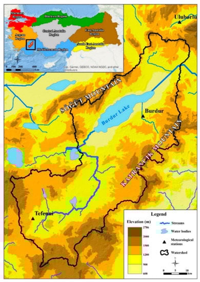
Figure 1.
Location of Burdur Lake in Turkey and the local watershed.
2.2. Data Source (Landsat5 TM, 7 ETM+, 8 OLI Data, NDVI Data, and Climate Data)
Burdur Lake is covered by Paths 178 and 179 and Row 34. By utilizing the GEE Landsat-hosted dataset, 570 scenes have been obtained from 1984 to 2019.
The Landsat images were collected from the Landsat 4–5 Thematic Mapper sensor (TM) [60], Landsat 7 Enhanced Thematic Mapper Plus (ETM+) [61], and Landsat 8 Operational Land Imager (OLI)/Thermal Infrared Sensor (TIRS) [62] instruments.
The 3-hourly Global Land Data Assimilation System (ERA5-Land) product [63], which ingests ground-based observational and satellite data, was used to collect the annual cumulative precipitation, annual cumulative evapotranspiration, albedo, radiation, and annual average temperature.
The data of the vegetation cover was obtained from the combined 16 days MODIS NDVI through the GEE platform [64]. The MODIS-NDVI data was only available from 2000 to 2019.
2.3. Surface Water Body Extraction
The detailed methodology consists of three stages as illustrated in Figure 2: Firstly, there are the Landsat 5, 7, and 8 images listed from the GEE datasets across the Burdur area since 1984 to 2019. A total of 883 images were collected from Landsat 5, 612 images were collected from Landsat 7, and 425 images were gathered from Landsat 8. Although the GEE provides the possibility of filtering and removing the low-quality images by shadows, snow, and clouds, all the images found were masked based on the study area. Analyzing the maximum obtainable images enhances the time series continuity. Therefore, during the exploration of the Landsat images, several Landsat tiles (tiles within Paths 178 and 179 and Row 34 based on the Landsat World Reference System WRS-2) were found mainly cloudy but not cloudy within the area of Burdur Lake. Thus, these Landsat tiles were utilized to support the continuity of the extracted time series.
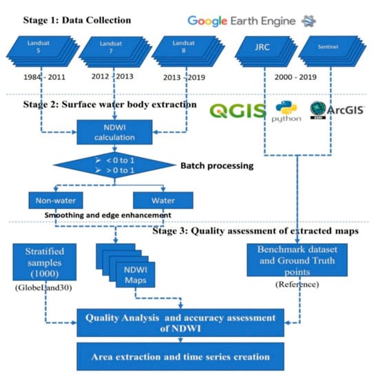
Figure 2.
A flowchart of the surface water extraction methodology using Landsat 5, 7, and 8 data utilizing GEE and the ArcGIS model builder iterator.
Secondly, the NDWI index was calculated from the various Landsat images in the GEE platform. Due to the limited 5 min of time processing and limited 5000 processing points provided by the GEE platform or temporal and spatial analysis, batch processing was implemented using Python within QGIS using the GEE plugin to overcome this problem. The NDWI method delineates the body of surface water by extracting the normalized difference between a reflected green visible band and a near-infrared band [65]. The NDWI index enhances the presence of surface water bodies and eliminates the presence of terrestrial vegetation and soil features. The NDWI index is calculated by using :
where
the NDWI is the normalized difference water index,
Green is the reflected green visible light and
the NIR is the reflected near-infrared energy.
Based on the data used in this analysis, the surface water bodies were extracted by Equations (2)–(4).
The postprocessing operations were performed in the second stage in the ArcGIS environment using a model builder iterator. The NDWI images were calculated on a pixel-by-pixel basis, then different thresholds were defined between the range of <0 and 0.1 to 1 based on different Landsat images and based on the visual interpretation. When the condition was met, the pixels were categorized as surface water and assigned 1 value. When the condition was not met, the pixels were categorized as non-surface water and assigned 0 value (5). Most of the threshold values were assigned 0 except some of the images were assigned 0.1 due to the complex image digital values. The different threshold values were assigned to distinguish the normal water bodies from water with high sand content and mudflats with high water content.
To extract the final vector polygon of Burdur Lake we proceeded as follows: (1) The results from the binary NDWI images were smoothed using a low-pass filter (kernel 3 by 3 pixels) to remove the noisy pixels and reduce the implication of abnormal cells. (2) The smoothed images again enhanced the subdued edges by utilizing a high-pass filter (kernel 3 by 3 pixels). (3) The results from the enhanced images were converted to a GIS vector format, and only the polygons of Burdur Lake were stored. The lake polygons were separated from other discrete plates by spatially intersecting them with the general diagonal line of Burdur Lake. A model builder with a vector iterator was built in ArcGIS, then ran over the polygons to extract only the Burdur Lake polygons. (4) Based on the visual interpretation using the satellite image as a base image for verification, several polygons were excluded from the list due to high gaps in the polygon area. Then, the area of each polygon was calculated as shown in Figure 3. (5) The monthly base time series were formed in Microsoft Excel using the PivotTable. The timeline of the collected data was classified into four seasons using the meteorological seasons in the Northern Hemisphere. The meteorological autumn (September, October, and November), winter (December, January, and February), spring (March, April, and May), and summer (June, July, and August) [66].
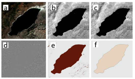
Figure 3.
Results of Burdur Lake mapping of each processing stage. (a) the original Landsat image, (b) the NDWI map of Burdur Lake, (c) the smoothed NDWI image using a low-pass filter, (d) the edge-enhanced NDWI image using high-pass filter, (e) the binary map of water and non-water areas, (f) final extracted vector polygon of the Burdur area.
2.4. Accuracy Assessment of Extracted Surface Water Data
This section aims to prove the efficiency of the proposed method of surface water body extraction and illustrates the quality of the extracted data of the lake borders. The process involves 3 datasets as follows:
- (1)
- The proposed dataset uses the raw Landsat images to extract the lake borders to monitor the degradation process. To generate a base for an accuracy assessment and to avoid any statistical misrepresentation of the location of assessment points, pixel-by-pixel accuracy assessment methods were employed. By applying the pixel-by-pixel accuracy assessment method, hundreds of thousands of pixels were taken around the coastline of the lake. A rectangle was drawn over the lake area and clipped the lake area from the Sentinel satellite image. The clipped image consists of 3588 rows and 3210 columns, which lead to producing 4,035,395 pixels. These pixels were converted to points. The points were used as a base to extract the pixels values from the NDWI images. The confusion matrix was calculated again using 4,035,395 pixels.
- (2)
- Lastly, the 4,035,395 points act as ground truth points to visually interpret the non-water and water areas based on the 10 m resolution Sentinel-2. Due to the limited temporal Sentinel-2 satellite images, we searched and matched between the images of the same month and year from two datasets (Sentinel images and our produced NDWI). The matching processing is to avoid the sensitivity and seasonality problem of the water area during the accuracy comparison. The found Sentinel images were for the years 2016, 2017, 2018, and 2019 and the 8, 9, 8, 9 months, respectively.
The confusion matrix was generated to compute the User Equation (5), Producer Equation (6), and Overall Accuracy Equation (7) [67]. In addition, Cohen’s Kappa index was calculated to measure the agreement among the two datasets [68]:
where TP = true positive value, FP = false positive value, TN = true negative value, and FN = false negative value.
2.5. Statistical Analysis
The extracted results from the Landsat images were analyzed using descriptive statistics and the Pearson correlation analysis [69]. Furthermore, a factor analysis was used to identify the sources of variation in the data. A factor analysis (FA) is a multivariate technique used to produce new uncorrelated variables using the original data values. A principal components analysis (PCA) is usually used to extract the factors from the correlation matrix of the selected variables. The extracted components are usually rotated to reduce the contribution of less significant variables [70,71]. The process will result in a few factors that account for the same amount of information as the original dataset.
3. Results and Discussion
3.1. Accuracy Assessment of Surface Water Map
The extracted results from the Landsat images were compared point-to-point with the Sentinel-2 images over the last four years in our time series duration (2016, 2017, 2018, and 2019). Table 1 presents each water and non-water point extracted from Sentinel-2 images and their User’s Accuracy, Producer’s Accuracy, as well as Overall Accuracy and the number of points in each category. The Overall Accuracy of our extraction methodology was more than 99%, the Producer’s Accuracy for non-water areas and water areas was more than 99%, and the User’s Accuracy was more than 99% for non-water areas and water areas over the years 2016, 2017, 2018, and 2019.

Table 1.
Accuracy assessment of the last 4 years of the Burdur NDWI area (2016, 2017, 2018, and 2019) based on the visual interpretation from Sentinel-2 images using the pixel-by-pixel method.
The obtained results show a high degree of accuracy for the proposed extraction method results in this study and the benchmark data. This high degree of accuracy is a supportive indicator of the quality of the extracted data and the employed methodology where the dissimilarity is reasonable since there should be a margin of error even in the benchmark dataset extraction methodology as well as the proposed method.
Ultimately, this assessment reflects the effectiveness and the simplicity of the proposed method, triggers the potential for publishing the data on an open-source platform, and paves the way for applying the same principle to other attractive geographical areas for further investigation.
3.2. Spatial and Temporal Changes of Burdur Lake Area from 1984 to 2019
The analysis of long-term, remotely-sensed data of Burdur Lake has shown that the water body of the lake has dramatically decreased from 1984 to 2019. The trend of the decrease in the lake area was observed by utilizing Landsat images at roughly five-year intervals. The follow-up of the changes in the area covering the lake was examined within seven periods as 1984–1990, 1995, 2000, 2005, 2010, 2015, 2019 as shown in Figure 4. As a result, the areal changes of Burdur Lake were determined, considering the periods as 206.6, 192.2, 172.9, 158, 156.8, 144.2, 135.8, 125.5 km2, respectively.
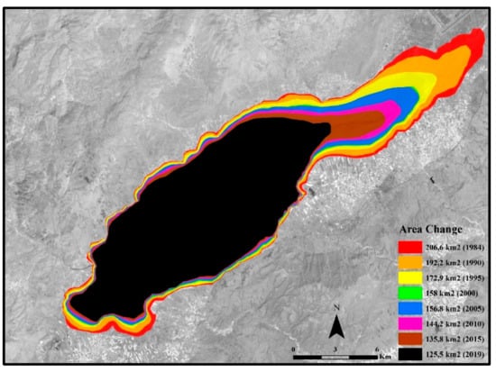
Figure 4.
The coastline and areal changes of Burdur Lake’s water body according to years.
Burdur Lake lies in a southwest-northeast direction, and the depth of the lake is shallower on the northeast side. For this reason, the maximum areal changes of the lake had taken place by 1984–2000, which is the first three periods on the northeast edge of the water body [72,73]. The radical reduction in the lake area led to a severe loss of wetland habitat, resulting in the drying up of shallow areas of great importance to waterfowl. Figure 5 shows the trend and temporal variation in the lake area between 1984 and 2019. It is obvious that during the thirty-four years, the lake area continually decreased except for the period between 2003 and 2004. Unfortunately, after 2006, the area continued to decrease with an almost fixed rate of reduction. The trend of the annual area shows the same reduction pattern after 2006 until 2019. Figure 5 indicates that the decrease in the lake area is ongoing and will lead to further reduction. According to the general trend of the lake, the annual reduction in the area is 2.35 km2 per year. In case the lake conditions persist, starting in 2019, the lake will lose half of its area in eight and a half years.
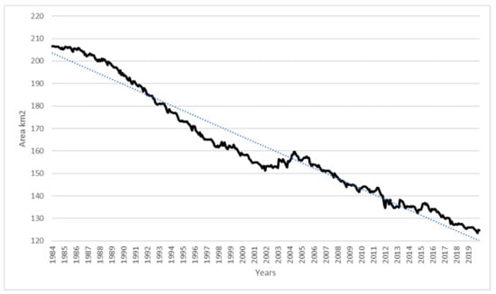
Figure 5.
The trend and temporal variation in the lake area between 1984 and 2019.
Moreover, the seasonal and annual redaction variation in the lake area between 1985 and 2019 are presented in Figure 6. Generally, the reduction in the lake area happened most of the time except the years 1985, 1998, 2002, 2003, 2004, and 2005, when the area of Burdur Lake increased annually to 0.39, 0.15, 1.4, 2.24, 0.83, and 0.36 km2, respectively. Between 2003 and 2006, the decrease in the area stopped and started to recover. The lake area slightly increased from 154 to 158 km2. The worst redaction was in 2011, where the area was reduced by 6.23 km2 in one year. Figure 6 also presents the seasonal variation in redactions. The two subfigures show that the redactions happened during the summer and autumn seasons, while in the winter and spring seasons, the lake gained some area over a few years especially after the year 2000. These outcomes indicate the strong linkage between the lake area and the rainy-snowy seasons as well as the source of lake water.
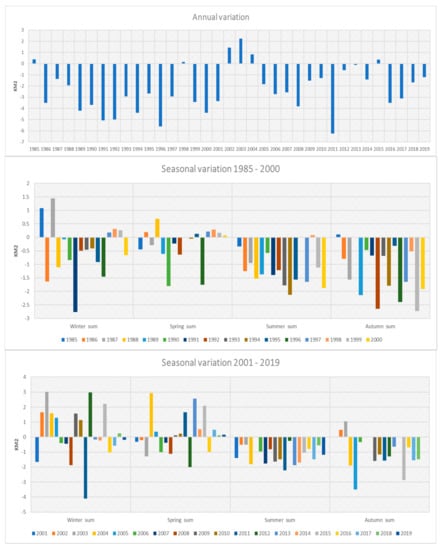
Figure 6.
Seasonal and annual temporal redaction variation between 1985 and 2000.
3.3. Descriptive Statistics of Climatological Data, Vegetation, and Temporal Area
The results for temperature, evaporation, precipitation, albedo, radiation, and the reduction of the lake area are summarized as a minimum, maximum, mean, and standard deviation (Table 2). The lowest average value was observed for evaporation, which was −0.002, and the highest average value was observed for radiation, which was 1.6478000. Furthermore, the standard deviation was low and acceptable, except radiation was high, which was 6,449,530. This was due to the seasonal variation as well as cloudy times. The collected data were further analyzed based on the season. The boxplot for the reduction of the area of the lake and selected variables are presented in Figure 7 showing the first, second (median), and third quartiles with minimum and maximum values. Figure 7 exhibits a very big fluctuation for the selected variables during the various season and within each season as well. The higher changes in the area of the lake may be attributed to the high changes in all selected meteorological parameters, especially in winter and spring. In summary, the selected variables behave differently during each season and between various seasons.
Table 2.
Minimum, maximum, mean, and standard deviations for the selected variables.
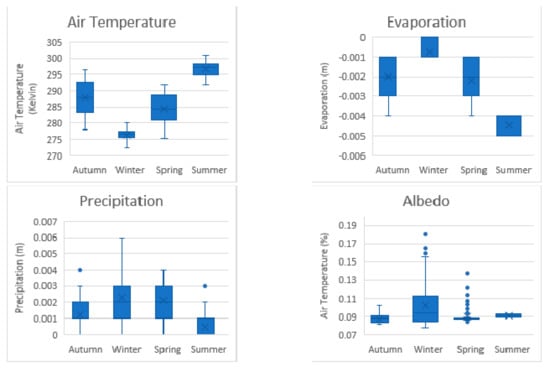
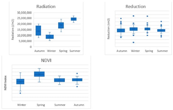
Figure 7.
Boxplot for the selected variables based on season.
3.4. Correlation Analysis
The relationship between selected variables (temperature, evaporation, precipitation, albedo, radiation, and NDVI) of the lake area was studied to understand the behavior of each variable in the presence of other variables. The correlation matrix for the coefficient of correlation is presented in Table 3. The correlation matrix showed a strong positive or negative significant relationship (p-value < 0.01 or p-value < 0.05) as presented in Table 3 between the reduction and the selected variables. Furthermore, a strong correlation was exhibited between various variables in the presence of other variables. In summary, the selected variables influence the reduction in the lake area directly during various seasons.
Table 3.
Correlation matrix for the selected variables.
3.5. Factor Analysis
The collected data were further analyzed to identify the amount of explained variation in the data. A factor analysis is a multivariate method used to describe the relationship between various selected variables which are highly correlated with a smaller number of new, uncorrelated variables called factors. A factor analysis is considered as a data reduction method that proposes how many variates are important to explain the observed variances in the data. The analysis was provided only three components which explain 82.15% of the total variation in the data. The contribution of each variable to each factor is represented by the coefficient associated with each variable in Equations (8)–(10):
The first factor (F1) explains more than 45% (45.06) of the total variation in the data, this contribution is mainly due to the difference between temperature, radiation, and from the other side evaporation and precipitation. The second factor (F2) explains 18.90% which is mainly due to the difference between vegetation cover (NDVI) and albedo, whilst the third factor (F3) explains only 18.19% of the total variation in the data which is due to the reduction in the area of the lake. The contribution of the selected variables in explaining the total variation during various seasons is represented in a boxplot as shown in Figure 8 showing the effect during various seasons. The values of the factors behave differently during various seasons. Furthermore, winter exhibited the highest fluctuation for factors 2 and 3 which is due to the NDVI, albedo, and reduction of the lake area. The lake is fed by rainfall of the basin, the rivers that flow into the lake, and groundwaters. Since there is no water flow out of the lake, water losses occur only through evaporation and infiltration [72]. The water level of the lake has decreased by 14 m, and the total volume of the lake has decreased by 38%. A high correlation was found between the decrease in the lake level and the temperature and total evaporation [73].
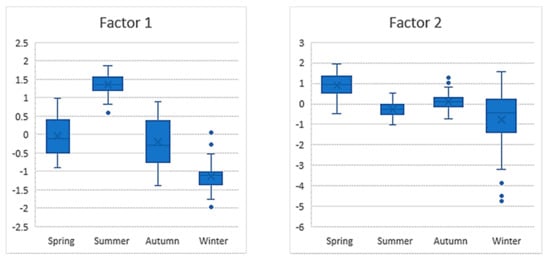
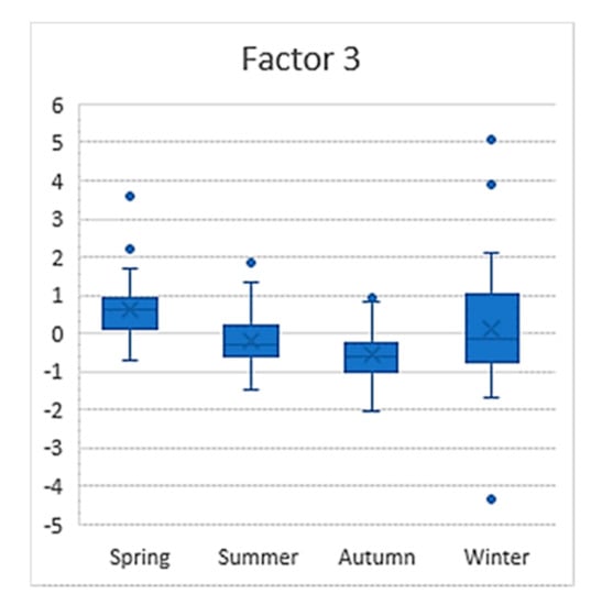
Figure 8.
Boxplot for the values of the extracted factors during various seasons.
According to some studies, the decreasing trend of the lake’s water level is rooted in increasing human activity in the Burdur Lake basin. Especially dams constructed on rivers feeding the lake to irrigate agricultural lands in the basin reduce the amount of water feeding the lake. Besides, excessive water consumption of the marble quarries in the basin is among the important reason for the water level decrease [74]. According to another study, the use of rivers feeding the lake for mains water and the use of groundwater for agriculture caused the water level of the lake to decrease [75]. In other words, the reasons for the decrease in the water level of the lake are the increase in water consumption due to the expansion of urban areas and agricultural lands in harmony with the population increase. In addition, because the area where the lake is located is tectonically active, the direction and drying of the underground waters due to the earthquakes may have caused the water level of the lake to decrease [76]. Figure 9 shows the relationship between the reduction in the area of the lake with the NDVI.
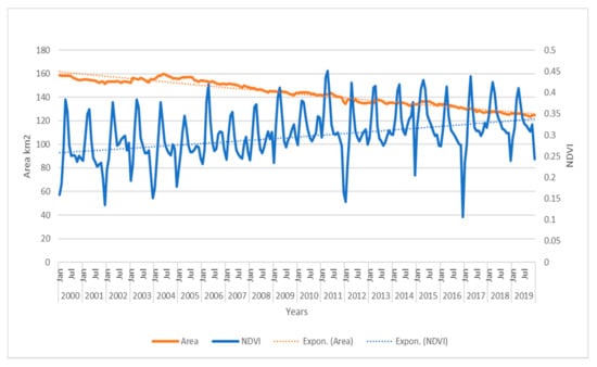
Figure 9.
The relationship between the reduction in the area of the lake and the NDVI index.
4. Conclusions
In this work, the relationship between selected meteorological variables and the reduction of the lake area was studied for 34 years between 1984 and 2019 to understand the behavior of each variable in the presence of other variables. A strong positive or negative correlation showed a significant relationship (p-value < 0.01 or p-value < 0.05) between the reduction of the lake area and the selected variables. Furthermore, a strong correlation is exhibited between various variables in the presence of other variables. In summary, the selected variables influence the reduction of lake area directly during various seasons. A factor analysis provided three components that explain 82.15%% of the total variation in the data. The contribution of each variable to each factor is represented by the coefficient associated with each variable. The first factor explains more than 45% (45.06) of the total variation in the data, this contribution is mainly due to the difference between temperature, radiation, and, from the other side, evaporation and precipitation. The second factor explains 18.90% which is mainly due to the variation of the vegetation cover (NDVI) and albedo, whilst the third factor explains only 18.19% of the total variation in the data, which is due to the reduction in the area of the lake. The values of the factors behave differently during various seasons. Furthermore, human activities such as agriculture and industry may contribute to the degradation rate of lake areas which may be considered in future work. In addition, the lake body area as a unit of measurement alone expresses the relative deterioration of the water volume in the lake, but the difference in the depth of the lake from one place to another can lead to a margin of error in the area of the lake body. Thus, solutions to this problem can be developed in future studies by linking the area extracted from satellite images with depth data, if available.
Author Contributions
Conceptualization, S.K.M.A., M.A., S.S.A.A. and A.F.M.A.; methodology S.K.M.A., M.A., S.S.A.A. and A.F.M.A.; writing—original draft preparation, S.K.M.A., S.S.A.A., E.T., K.H.A., A.M.H. and A.F.M.A.; writing—review and editing, M.A., S.S.A.A. and A.F.M.A.; visualization, S.K.M.A., M.A. and A.F.M.A.; supervision, A.M.H.; project administration, S.K.M.A.; funding acquisition, K.H.A. All authors have read and agreed to the published version of the manuscript.
Funding
This research received no external funding.
Data Availability Statement
Data are available at: https://developers.google.com/earth-engine/datasets/catalog/LANDSAT_LT05_C01_T1; https://developers.google.com/earth-engine/datasets/catalog/LANDSAT_LE07_C01_T1_SR; https://developers.google.com/earth-engine/datasets/catalog/LANDSAT_LC08_C01_T1; https://developers.google.com/earth-engine/datasets/catalog/ECMWF_ERA5_LAND_MONTHLY; https://developers.google.com/earth-engine/datasets/catalog/MODIS_MCD43A4_006_NDVI?hl (all accessed on 16 November 2021).
Conflicts of Interest
The authors declare no conflict of interest.
Abbreviations
| GEE | Google Earth Engine |
| NDWI | Normalized Difference Water Index |
| NDVI | Normalized Difference Vegetation Index |
| TM | Thematic Mapper |
| ETM+ | Enhanced Thematic Mapper Plus |
| OLI | Operational Land Imager |
| TIRS | Thermal Infrared Sensor |
| FA | Factor Analysis |
| PCA | Principal Components Analysis |
| WRS2 | World Reference System |
References
- Duran-Encalada, J.A.; Paucar-Caceres, A.; Bandala, E.R.; Wright, G.H. The impact of global climate change on water quantity and quality: A system dynamics approach to the US–Mexican transborder region. Eur. J. Oper. Res. 2017, 256, 16. [Google Scholar] [CrossRef] [Green Version]
- Hall, J.W.; Grey, D.; Garrick, D.; Fung, F.; Brown, C.; Dadson, S.J.; Sadoff, C.W. Coping with the curse of freshwater variability. Science 2014, 346, 429–430. [Google Scholar] [CrossRef] [PubMed]
- Worden, J.; de Beurs, K.M. Surface water detection in the Caucasus. Int. J. Appl. Earth Obs. Geoinf. 2020, 91, 102159. [Google Scholar] [CrossRef]
- Rickert, B.; Berg, H.V.D.; Bekure, K.; Girma, S.; Husman, A.M.D.R. Including aspects of climate change into water safety planning: Literature review of global experience and case studies from Ethiopian urban supplies. Int. J. Hyg. Environ. Health 2019, 222, 744–755. [Google Scholar] [CrossRef]
- WHO. Climate-Resilient Water Safety Plans: Managing Health Risks Associated with Climate Variability and Change; World Health Organization: Geneva, Switzerland, 2017; Available online: https://apps.who.int/iris/handle/10665/258722 (accessed on 5 August 2021).
- Dai, A. Increasing drought under global warming in observations and models. Nat. Clim. Chang. 2013, 3, 52–58. [Google Scholar] [CrossRef]
- Ulutaş, K.; Pekey, H.; Demir, S.; Dinçer, F. The Impact of Environmental Odor, near the Waste Water Treatment Plant on the Urban Life Quality. In Proceedings of the VII. Ulusal Hava Kirliliği Ve Kontrolü Sempozyumu, Antalya, Turkey, 1–3 November 2017. [Google Scholar]
- Chenoweth, J.; Hadjinicolaou, P.; Bruggeman, A.; Lelieveld, J.; Levin, Z.; Lange, M.A.; Xoplaki, E.; Hadjikakou, M. Impact of climate change on the water resources of the eastern Mediterranean and Middle East region: Modeled 21st century changes and implications. Water Resour. Res. 2011, 47, W06506. [Google Scholar] [CrossRef]
- Lacirignola, C.; Capone, R.; Debs, P.; El Bilali, H.; Bottalico, F. Natural Resources – Food Nexus: Food-Related Environmental Footprints in the Mediterranean Countries. Front. Nutr. 2014, 1, 2296–861X. [Google Scholar] [CrossRef] [Green Version]
- Gorguner, M.; Kavvas, M.L. Modeling impacts of future climate change on reservoir storages and irrigation water demands in a Mediterranean basin. Sci. Total Environ. 2020, 748, 141246. [Google Scholar] [CrossRef]
- Yilmaz, K.K.; Yazicigil, H. Potential Impacts of Climate Change on Turkish Water Resources: A Review. Clim. Chang. Its Eff. Water Resour. 2011, 3, 105–114. [Google Scholar]
- Adaman, F.; Hakyemez, S.; Özkaynak, B. The Political Ecology of a Ramsar Site Conservation Failure: The Case of Burdur Lake, Turkey. Environ. Plan. C Gov. Policy 2009, 27, 783–800. [Google Scholar] [CrossRef]
- Varol, S.; Davraz, A. Evaluation of the groundwater quality with WQI (Water Quality Index) and multivariate analysis: A case study of the Tefenni plain (Burdur/Turkey). Environ. Earth Sci. 2014, 73, 1725–1744. [Google Scholar] [CrossRef]
- Walker, J.J.; Soulard, C.E.; Petrakis, R.E. Integrating stream gage data and Landsat imagery to complete time-series of surface water extents in Central Valley, California. Int. J. Appl. Earth Obs. Geoinf. 2019, 84, 101973. [Google Scholar] [CrossRef]
- Davraz, A.; Şener, E.; Sener, S. Evaluation of climate and human effects on the hydrology and water quality of Burdur Lake, Turkey. J. Afr. Earth Sci. 2019, 158, 103569. [Google Scholar] [CrossRef]
- Liu, J.; Heiskanen, J.; Maeda, E.E.; Pellikka, P.K. Burned area detection based on Landsat time series in savannas of southern Burkina Faso. Int. J. Appl. Earth Obs. Geoinf. 2018, 64, 210–220. [Google Scholar] [CrossRef] [Green Version]
- Bioresita, F.; Puissant, A.; Stumpf, A.; Malet, J.-P. A Method for Automatic and Rapid Mapping of Water Surfaces from Sentinel-1 Imagery. Remote Sens. 2018, 10, 217. [Google Scholar] [CrossRef] [Green Version]
- Pham-Duc, B.; Prigent, C.; Aires, F. Surface Water Monitoring within Cambodia and the Vietnamese Mekong Delta over a Year, with Sentinel-1 SAR Observations. Water 2017, 9, 366. [Google Scholar] [CrossRef] [Green Version]
- Feyisa, G.L.; Meilby, H.; Fensholt, R.; Proud, S.R. Automated Water Extraction Index: A new technique for surface water mapping using Landsat imagery. Remote Sens. Environ. 2014, 140, 23–35. [Google Scholar] [CrossRef]
- Huang, Y. Advances in Artificial Neural Networks–Methodological Development and Application. Algorithms 2009, 2, 973–1007. [Google Scholar] [CrossRef]
- Hassan-Esfahani, L.; Torres-Rua, A.; Jensen, A.; McKee, M. Assessment of Surface Soil Moisture Using High-Resolution Multi-Spectral Imagery and Artificial Neural Networks. Remote Sens. 2015, 7, 2627–2646. [Google Scholar] [CrossRef] [Green Version]
- Shu, C.; Burn, D.H. Artificial neural network ensembles and their application in pooled flood frequency analysis. Water Resour. Res. 2004, 40, W09301. [Google Scholar] [CrossRef] [Green Version]
- Mohammadpour, R.; Shaharuddin, S.; Chang, C.K.; Zakaria, N.A.; Ab Ghani, A.; Chan, N.W. Prediction of water quality index in constructed wetlands using support vector machine. Environ. Sci. Pollut. Res. 2014, 22, 6208–6219. [Google Scholar] [CrossRef]
- Yoshioka, M.; Fujinaka, T.; Omatu, S. SAR image classification by support vector machine. In Image Processing for Remote Sensing; CRC Press: Boca Raton, FL, USA, 2007. [Google Scholar]
- Liong, S.-Y.; Sivapragasam, C. FLOOD STAGE FORECASTING WITH SUPPORT VECTOR MACHINES. JAWRA J. Am. Water Resour. Assoc. 2002, 38, 173–186. [Google Scholar] [CrossRef]
- Naghibi, S.A.; Ahmadi, K.; Daneshi, A. Application of Support Vector Machine, Random Forest, and Genetic Algorithm Optimized Random Forest Models in Groundwater Potential Mapping. Water Resour. Manag. 2017, 31, 2761–2775. [Google Scholar] [CrossRef]
- Ding, J.; Jiang, Y.; Fu, L.; Liu, Q.; Peng, Q.; Kang, M. Impacts of Land Use on Surface Water Quality in a Subtropical River Basin: A Case Study of the Dongjiang River Basin, Southeastern China. Water 2015, 7, 4427–4445. [Google Scholar] [CrossRef] [Green Version]
- Feng, Q.; Liu, J.; Gong, J. Urban Flood Mapping Based on Unmanned Aerial Vehicle Remote Sensing and Random Forest Classifier—A Case of Yuyao, China. Water 2015, 7, 1437–1455. [Google Scholar] [CrossRef]
- Liu, R.; Chen, Y.; Wu, J.; Gao, L.; Barrett, D.; Xu, T.; Li, X.; Li, L.; Huang, C.; Yu, J. Integrating Entropy-Based Naïve Bayes and GIS for Spatial Evaluation of Flood Hazard. Risk Anal. 2016, 37, 756–773. [Google Scholar] [CrossRef]
- Pernkopf, F. Detection of surface defects on raw steel blocks using Bayesian network classifiers. Pattern Anal. Appl. 2004, 7, 333–342. [Google Scholar] [CrossRef]
- Mueller, N.; Lewis, A.; Roberts, D.; Ring, S.; Melrose, R.; Sixsmith, J.; Lymburner, L.; McIntyre, A.; Tan, P.; Curnow, S.; et al. Water observations from space: Mapping surface water from 25 years of Landsat imagery across Australia. Remote Sens. Environ. 2015, 174, 341–352. [Google Scholar] [CrossRef] [Green Version]
- Xu, H. Modification of normalised difference water index (NDWI) to enhance open water features in remotely sensed imagery. Int. J. Remote Sens. 2006, 27, 3025–3033. [Google Scholar] [CrossRef]
- Chowdary, V.; Chandran, R.V.; Neeti, N.; Bothale, R.; Srivastava, Y.; Ingle, P.; Ramakrishnan, D.; Dutta, D.; Jeyaram, A.; Sharma, J.; et al. Assessment of surface and sub-surface waterlogged areas in irrigation command areas of Bihar state using remote sensing and GIS. Agric. Water Manag. 2008, 95, 754–766. [Google Scholar] [CrossRef]
- Huang, W.; DeVries, B.; Huang, C.; Lang, M.W.; Jones, J.W.; Creed, I.F.; Carroll, M.L. Automated Extraction of Surface Water Extent from Sentinel-1 Data. Remote Sens. 2018, 10, 797. [Google Scholar] [CrossRef] [Green Version]
- Kumar, L.; Mutanga, O. Google Earth Engine Applications Since Inception: Usage, Trends, and Potential. Remote Sens. 2018, 10, 1509. [Google Scholar] [CrossRef] [Green Version]
- Alademomi, A.S.; Okolie, C.J.; Daramola, O.E.; Agboola, R.O.; Salami, T.J. Assessing the Relationship of LST, NDVI and EVI with Land Cover Changes in the Lagos Lagoon Environment. Quaest. Geogr. 2020, 39, 87–109. [Google Scholar] [CrossRef]
- Ghaderpour, E.; Ben Abbes, A.; Rhif, M.; Pagiatakis, S.D.; Farah, I.R. Non-stationary and unequally spaced NDVI time series analyses by the LSWAVE software. Int. J. Remote Sens. 2019, 41, 2374–2390. [Google Scholar] [CrossRef]
- Nanzad, L.; Zhang, J.; Tuvdendorj, B.; Nabil, M.; Zhang, S.; Bai, Y. NDVI anomaly for drought monitoring and its correlation with climate factors over Mongolia from 2000 to 2016. J. Arid. Environ. 2019, 164, 69–77. [Google Scholar] [CrossRef]
- Gupta, S.K.; Pandey, A.C. Spectral aspects for monitoring forest health in extreme season using multispectral imagery. Egypt. J. Remote Sens. Space Sci. 2021, in press. [Google Scholar] [CrossRef]
- Ali, M.I.; Dirawan, G.D.; Hasim, A.H.; Abidin, M.R. Detection of Changes in Surface Water Bodies Urban Area with NDWI and MNDWI Methods. Int. J. Adv. Sci. Eng. Inf. Technol. 2019, 9, 946. [Google Scholar] [CrossRef] [Green Version]
- Wang, L.; Jia, Y.; Yao, Y.; Xu, D. Accuracy Assessment of Land Use Classification Using Support Vector Machine and Neural Network for Coal Mining Area of Hegang City, China. Nat. Environ. Pollut. Technol. 2019, 18, 335–341. [Google Scholar]
- Sarp, G.; Ozcelik, M. Water body extraction and change detection using time series: A case study of Lake Burdur, Turkey. J. Taibah Univ. Sci. 2017, 11, 381–391. [Google Scholar] [CrossRef] [Green Version]
- Wulder, M.A.; Loveland, T.R.; Roy, D.P.; Crawford, C.J.; Masek, J.G.; Woodcock, C.E.; Allen, R.G.; Anderson, M.C.; Belward, A.S.; Cohen, W.B.; et al. Current status of Landsat program, science, and applications. Remote Sens. Environ. 2019, 225, 127–147. [Google Scholar] [CrossRef]
- Zhu, Z.; Wulder, M.; Roy, D.P.; Woodcock, C.E.; Hansen, M.C.; Radeloff, V.C.; Healey, S.P.; Schaaf, C.; Hostert, P.; Strobl, P.; et al. Benefits of the free and open Landsat data policy. Remote Sens. Environ. 2019, 224, 382–385. [Google Scholar] [CrossRef]
- Popkin, G. Technology and satellite companies open up a world of data. Nature 2018, 557, 745–747. [Google Scholar] [CrossRef]
- Gorelick, N.; Hancher, M.; Dixon, M.; Ilyushchenko, S.; Thau, D.; Moore, R. Google Earth Engine: Planetary-scale geospatial analysis for everyone. Remote Sens. Environ. 2017, 202, 18–27. [Google Scholar] [CrossRef]
- Thieme, A.; Yadav, S.; Oddo, P.; Fitz, J.M.; McCartney, S.; King, L.; Keppler, J.; McCarty, G.W.; Hively, W.D. Using NASA Earth observations and Google Earth Engine to map winter cover crop conservation performance in the Chesapeake Bay watershed. Remote Sens. Environ. 2020, 248, 111943. [Google Scholar] [CrossRef]
- Pan, L.; Xia, H.; Yang, J.; Niu, W.; Wang, R.; Song, H.; Guo, Y.; Qin, Y. Mapping cropping intensity in Huaihe basin using phenology algorithm, all Sentinel-2 and Landsat images in Google Earth Engine. Int. J. Appl. Earth Obs. Geoinf. 2021, 102, 102376. [Google Scholar] [CrossRef]
- Chen, B.; Xiao, X.; Li, X.; Pan, L.; Doughty, R.; Ma, J.; Dong, J.; Qin, Y.; Zhao, B.; Wu, Z.; et al. A mangrove forest map of China in 2015: Analysis of time series Landsat 7/8 and Sentinel-1A imagery in Google Earth Engine cloud computing platform. ISPRS J. Photogramm. Remote Sens. 2017, 131, 104–120. [Google Scholar] [CrossRef]
- Lee, J.S.H.; Wich, S.; Widayati, A.; Koh, L.P. Detecting industrial oil palm plantations on Landsat images with Google Earth Engine. Remote Sens. Appl. Soc. Environ. 2016, 4, 219–224. [Google Scholar] [CrossRef] [Green Version]
- Johansen, K.; Phinn, S.; Taylor, M. Mapping woody vegetation clearing in Queensland, Australia from Landsat imagery using the Google Earth Engine. Remote Sens. Appl. Soc. Environ. 2015, 1, 36–49. [Google Scholar] [CrossRef]
- Duan, Q.; Tan, M.; Guo, Y.; Wang, X.; Xin, L. Understanding the Spatial Distribution of Urban Forests in China Using Sentinel-2 Images with Google Earth Engine. Forests 2019, 10, 729. [Google Scholar] [CrossRef] [Green Version]
- Wang, X.; Xiao, X.; Zou, Z.; Hou, L.; Qin, Y.; Dong, J.; Doughty, R.; Chen, B.; Zhang, X.; Chen, Y.; et al. Mapping coastal wetlands of China using time series Landsat images in 2018 and Google Earth Engine. ISPRS J. Photogramm. Remote Sens. 2020, 163, 312–326. [Google Scholar] [CrossRef]
- Cao, W.; Zhou, Y.; Li, R.; Li, X. Mapping changes in coastlines and tidal flats in developing islands using the full time series of Landsat images. Remote Sens. Environ. 2020, 239, 111665. [Google Scholar] [CrossRef]
- Wang, Y.; Ma, J.; Xiao, X.; Wang, X.; Dai, S.; Zhao, B. Long-Term Dynamic of Poyang Lake Surface Water: A Mapping Work Based on the Google Earth Engine Cloud Platform. Remote Sens. 2019, 11, 313. [Google Scholar] [CrossRef] [Green Version]
- Deng, Y.; Jiang, W.; Tang, Z.; Ling, Z.; Wu, Z. Long-Term Changes of Open-Surface Water Bodies in the Yangtze River Basin Based on the Google Earth Engine Cloud Platform. Remote Sens. 2019, 11, 2213. [Google Scholar] [CrossRef] [Green Version]
- Nguyen, U.N.T.; Pham, L.T.H.; Dang, T.D. An automatic water detection approach using Landsat 8 OLI and Google Earth Engine cloud computing to map lakes and reservoirs in New Zealand. Environ. Monit. Assess. 2019, 191, 1–12. [Google Scholar] [CrossRef]
- Bostan, H. Türkiye’de İç Göçlerin Toplumsal Yapıda Neden Olduğu Değişimler, Meydana Getirdiği Sorunlar ve Çözüm Önerileri. J. Geogr. 2020, 1, 1–16. [Google Scholar] [CrossRef]
- Öztürk, M.; Çetinkaya, G.; Aydın, S. Climate Types of Turkey According to Köppen-Geiger Climate Classification. Istanbul Univ. J. Geogr. 2017, 2017, 17–27. [Google Scholar] [CrossRef]
- USGS. USGS Landsat 5 TM Collection 1 Tier 1 Raw Scenes. Google Earth Engine. 2021. Available online: https://developers.google.com/earth-engine/datasets/catalog/LANDSAT_LT05_C01_T1 (accessed on 5 July 2021).
- USGS. USGS Landsat 7 Surface Reflectance Tier 1. Google Earth Engine. 2021. Available online: https://developers.google.com/earth-engine/datasets/catalog/LANDSAT_LE07_C01_T1_SR (accessed on 5 July 2021).
- USGS. USGS Landsat 8 Collection 1 Tier 1 Raw Scenes. Google Earth Engine. 2021. Available online: https://developers.google.com/earth-engine/datasets/catalog/LANDSAT_LC08_C01_T1 (accessed on 5 July 2021).
- USGS. ERA5-Land Monthly Averaged-ECMWF Climate Reanalysis. Google Earth Engine. 2021. Available online: https://developers.google.com/earth-engine/datasets/catalog/ECMWF_ERA5_LAND_MONTHLY#description (accessed on 5 July 2021).
- USGS. MODIS Combined 16-Day NDVI. Google Earth Engine. 2021. Available online: https://developers.google.com/earth-engine/datasets/catalog/MODIS_MCD43A4_006_NDVI?hl=en (accessed on 5 July 2021).
- McFeeters, S.K. The use of the Normalized Difference Water Index (NDWI) in the delineation of open water features. Int. J. Remote Sens. 1996, 17, 1425–1432. [Google Scholar] [CrossRef]
- NOAA. Meteorological Versus Astronomical Seasons. 2016. Available online: https://www.ncei.noaa.gov/news/meteorological-versus-astronomical-seasons (accessed on 9 September 2021).
- Stehman, S.V. Estimating area and map accuracy for stratified random sampling when the strata are different from the map classes. Int. J. Remote Sens. 2014, 35, 4923–4939. [Google Scholar] [CrossRef]
- McHugh, M.L. Interrater reliability: The kappa statistic. Biochem. Med. 2012, 22, 276–282. [Google Scholar] [CrossRef]
- Alkarkhi, A.F.M.; Low, H.C. Elementary Statistics for Technologist; Penerbit Universiti Sains Malaysia: Penang, Malaysia, 2012. [Google Scholar]
- Alkarkhi, A.F.M.; Ismail, N.; Ahmed, A.; Easa, A.M. Analysis of heavy metal concentrations in sediments of selected estuaries of Malaysia—a statistical assessment. Environ. Monit. Assess. 2008, 153, 179–185. [Google Scholar] [CrossRef]
- Yusup, Y.; Alqaraghuli, W.A.A.; Alkarkhi, A.F.M. Factor analysis and back trajectory of PM and its metal constituents. Environ. Forensics 2016, 17, 319–337. [Google Scholar] [CrossRef]
- Ministry of Development, Burdur Gölü’nün Sorunları, Çözümleri, Yönetimi ve Ekonomik Potansiyeli; Ministry of Development: Burdur, Turkey, 2012.
- Gözükara, G.; Altunbaş, S.; Sarı, M. Burdur Gölü’ndeki seviye değişimi sonucunda ortaya çıkan lakustrin materyalin zamansal ve mekansal değişimi. Anadolu J. Agric. Sci. 2019, 34, 386–396. [Google Scholar] [CrossRef] [Green Version]
- Kaya, L.G.; Yücedağ, C.; Duruşkan, Ö. Burdur Gölü Havzasının Çevresel Açıdan İrdelenmesi. Mehmet Akif Ersoy Üniversitesi Fen Bilim. Enstitüsü Derg. 2015, 6, 6–10. [Google Scholar] [CrossRef] [Green Version]
- Ataol, M. Burdur Gölü’nde Seviye Değişimleri. Coğrafi Bilim. Derg. 2010, 8, 77–92. [Google Scholar] [CrossRef]
- Şahin, Ş.; Beyhan, M.; Keskin, E.; Harman, B.İ. Burdur Çevresinde Yaşanan Depremler ve Çevre Sorunları. I. Burdur Sempozyumu Turk. 2004, 910–914. [Google Scholar]
Publisher’s Note: MDPI stays neutral with regard to jurisdictional claims in published maps and institutional affiliations. |
© 2021 by the authors. Licensee MDPI, Basel, Switzerland. This article is an open access article distributed under the terms and conditions of the Creative Commons Attribution (CC BY) license (https://creativecommons.org/licenses/by/4.0/).