
Land Use and Land Cover Change in the Yellow River Basin from 1980 to 2015 and Its Impact on the Ecosystem Services


Abstract
:1. Introduction
2. Study Area and Methods
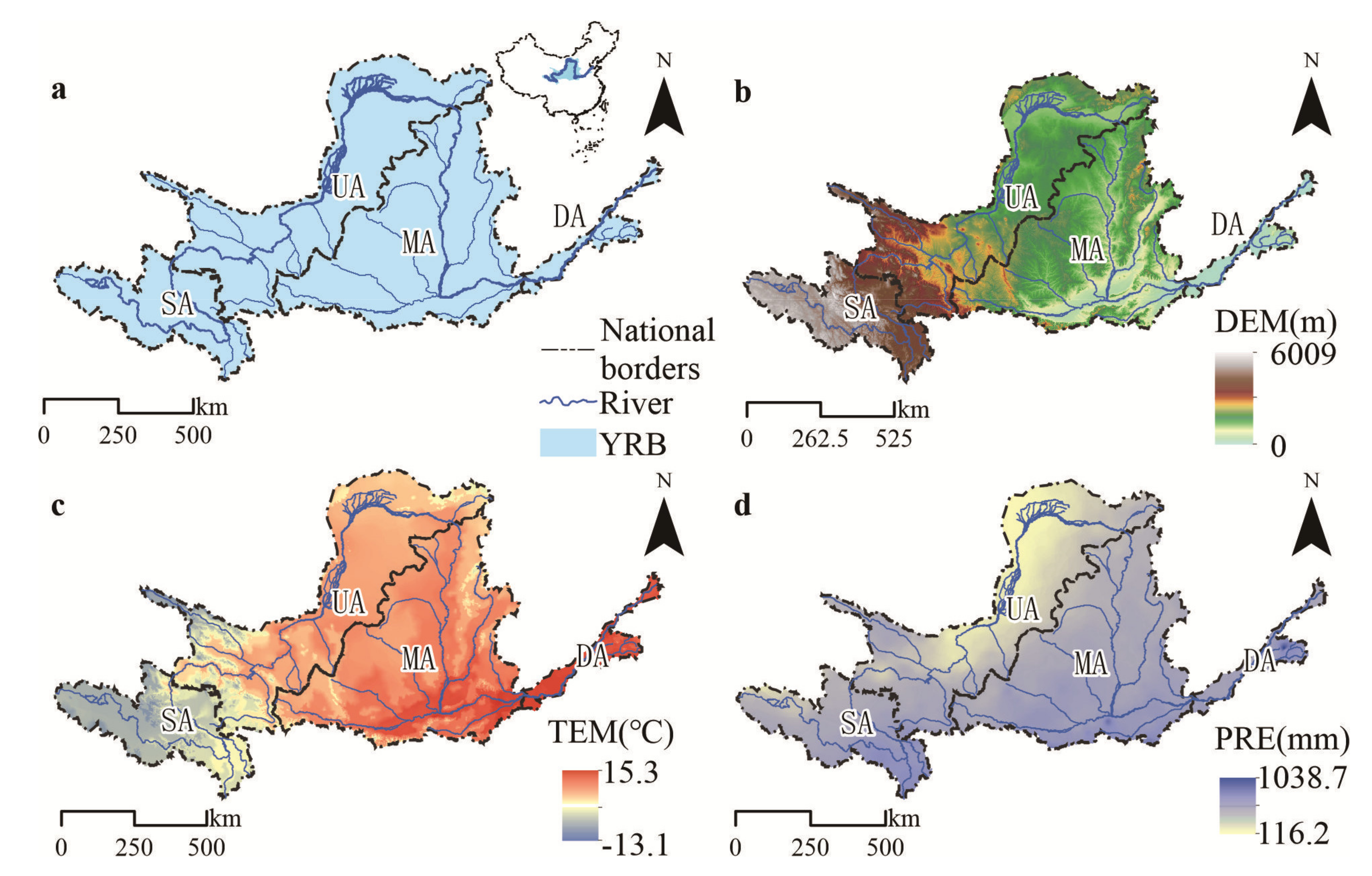
2.1. Study Area
2.2. Data Sources
2.3. LULC Change Transition Analysis
2.4. Estimation of Human-Induced LC Changes
2.5. Estimation of ESV
2.6. Elasticity-Sensitivity Analysis
3. Results
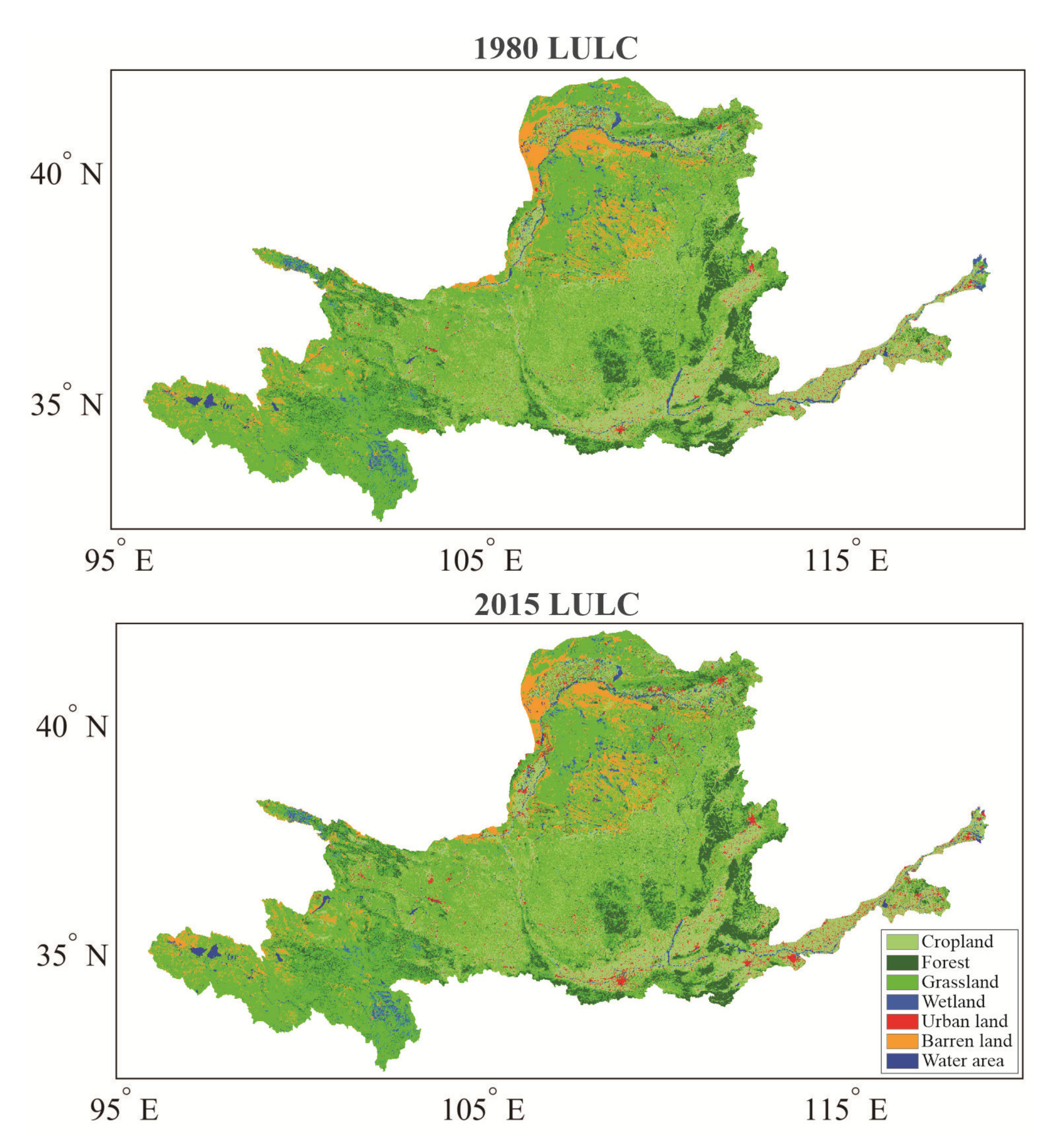
3.1. LULC Areas from 1980 to 2015
3.1.1. Basin Scale
3.1.2. Watershed Scale
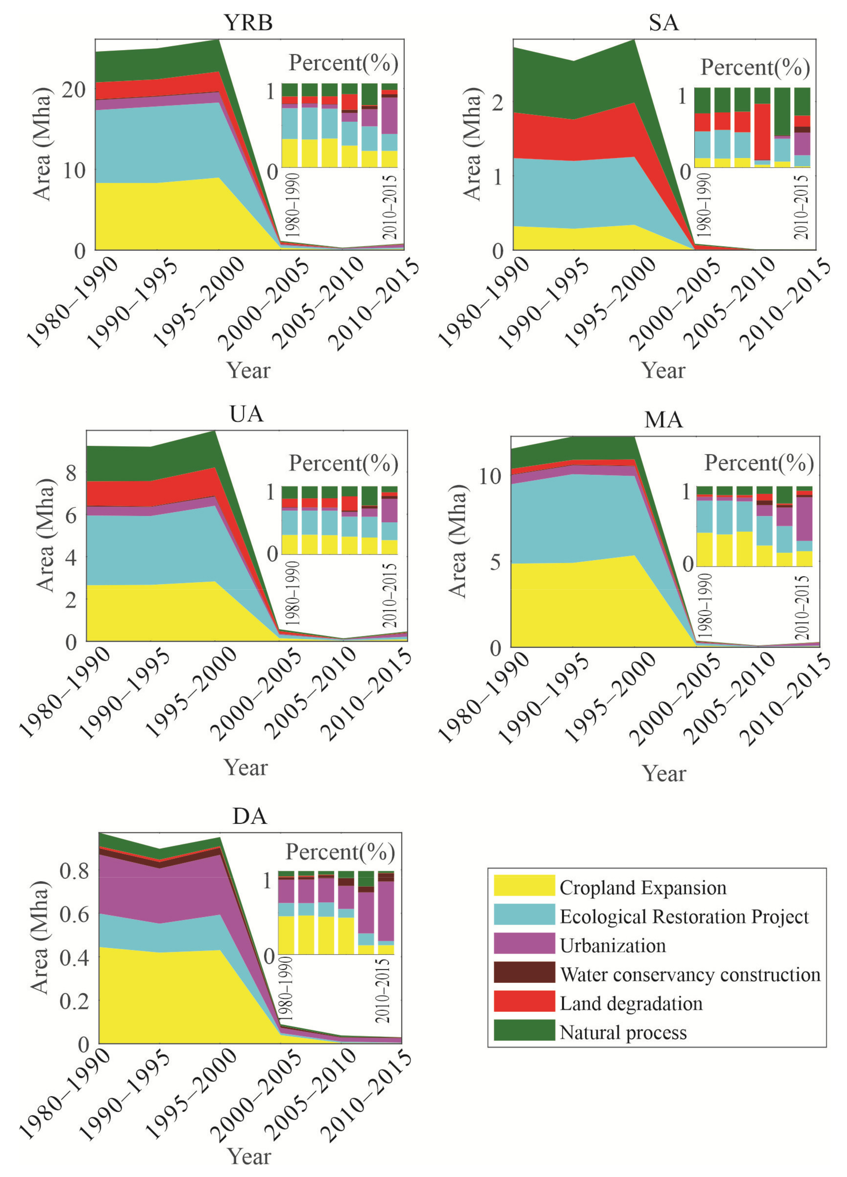
3.2. LULC Change Area from 1980 to 2015
3.2.1. Basin Scale
3.2.2. Watershed Scale
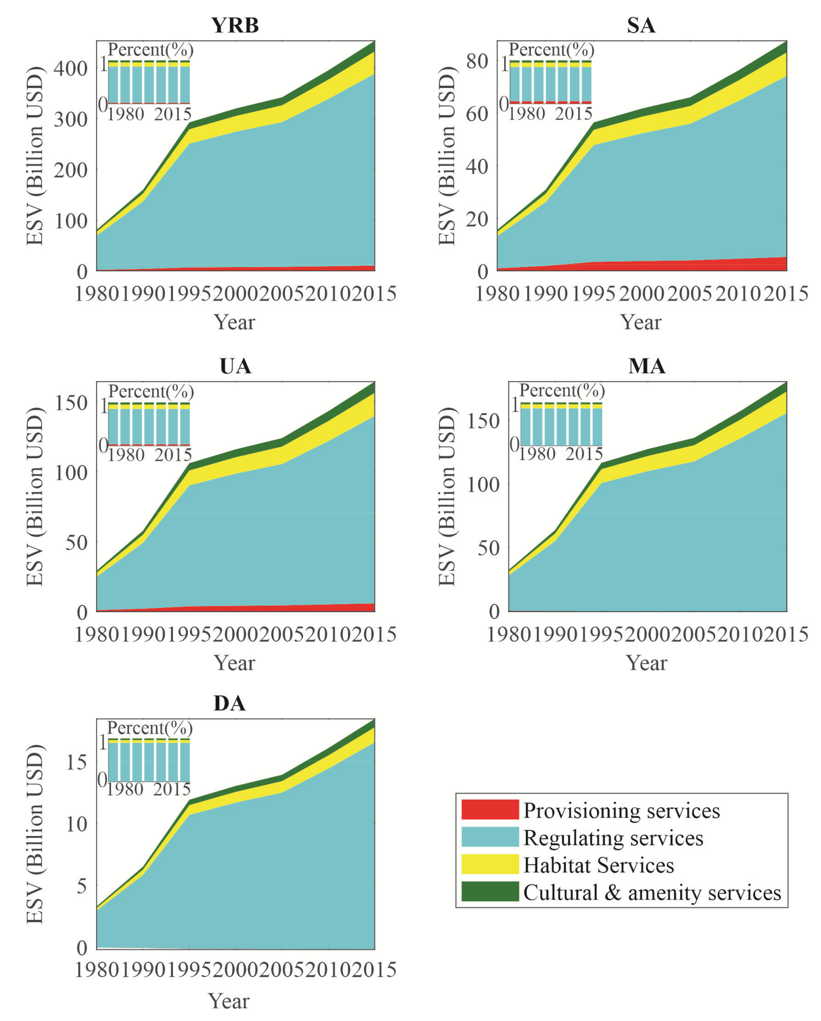
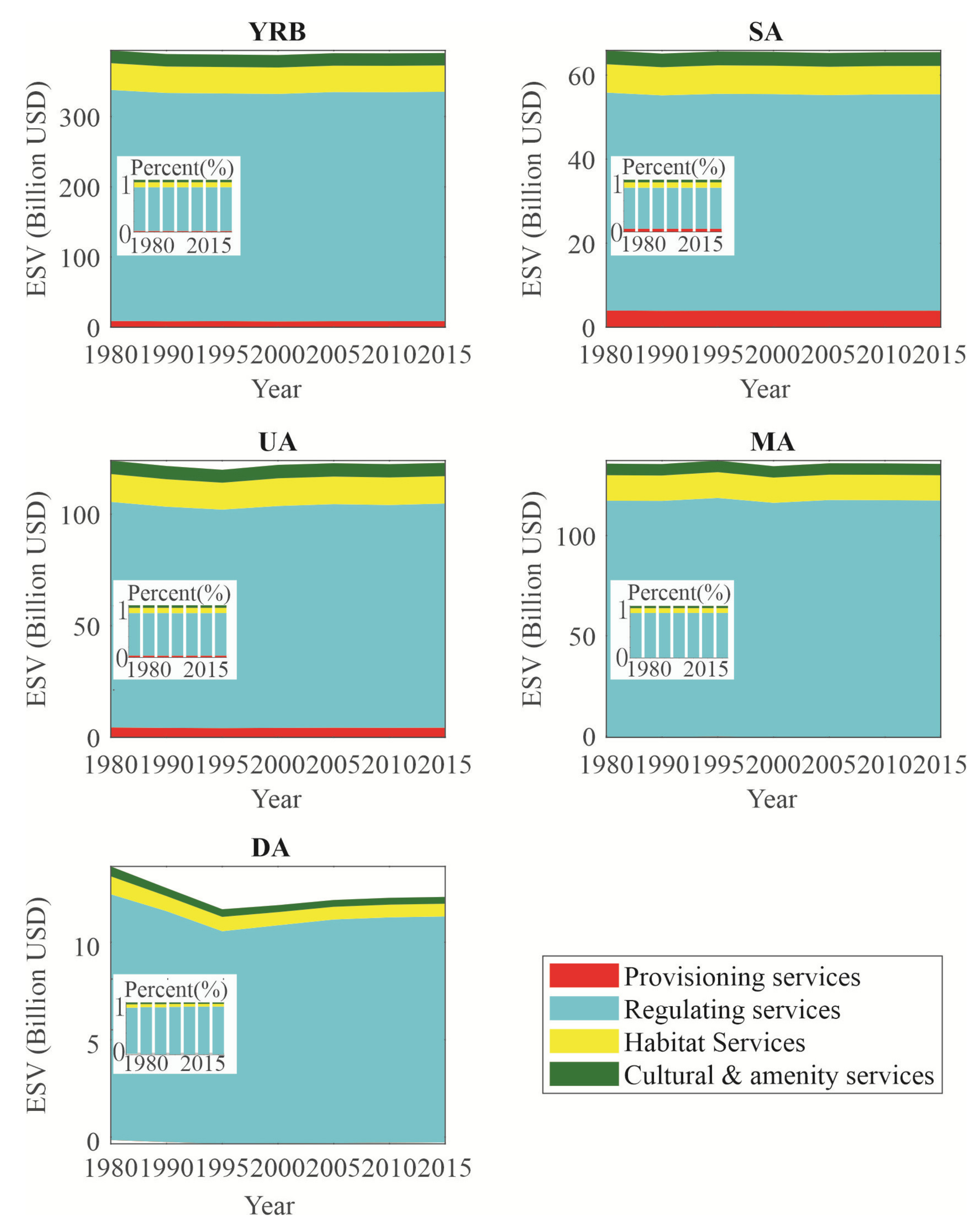
3.3. ESV from 1980 to 2015
3.3.1. Basin Scale
3.3.2. Watershed Scale
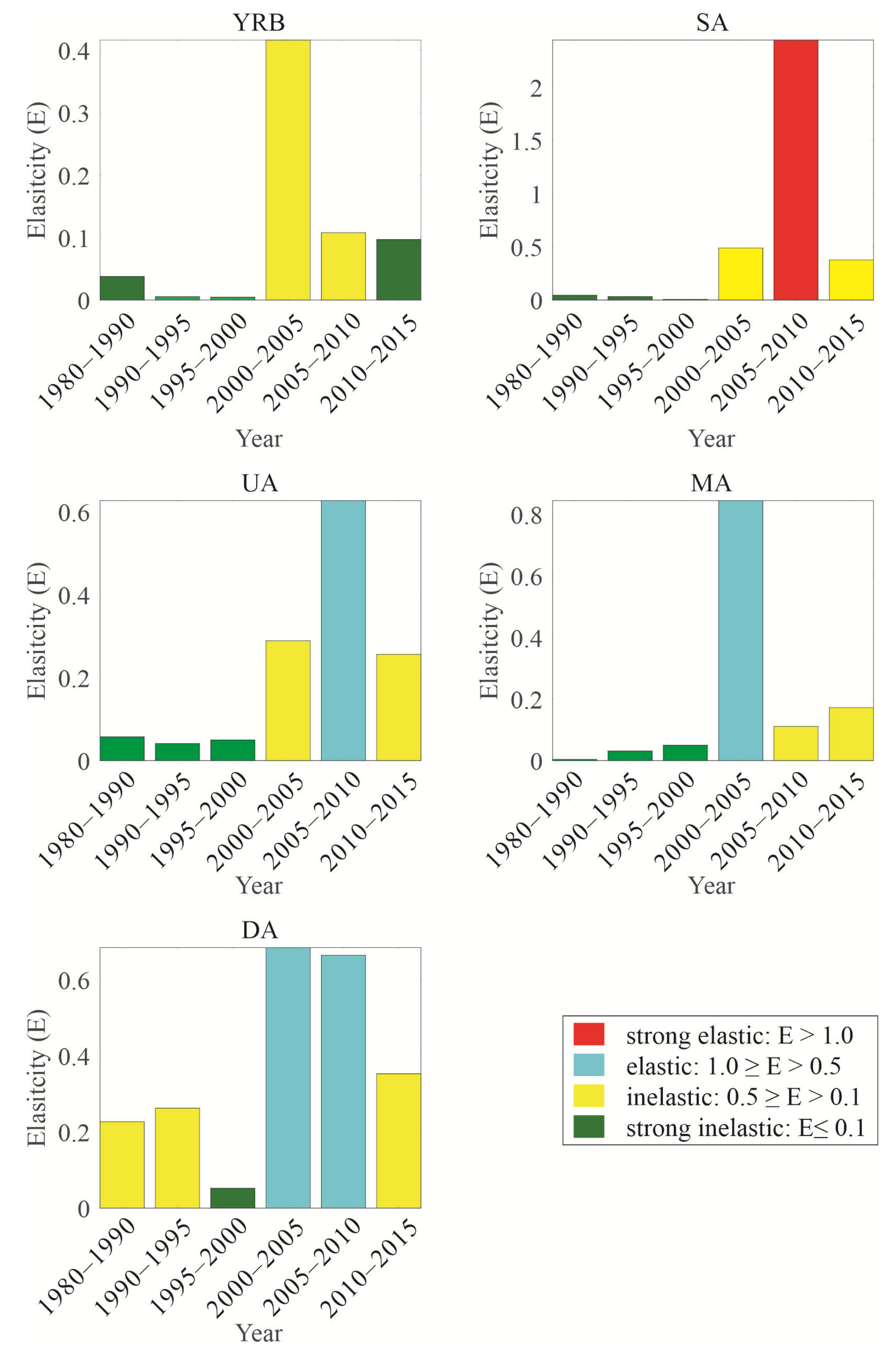
3.4. Elasticity of ESV Changes in Relation to LUCC
4. Discussions
4.1. Implications for Sustainable Development
4.2. Uncertainties in ESV Assessment
4.3. Limitations
5. Conclusions
Author Contributions
Funding
Acknowledgments
Conflicts of Interest
Abbreviations
Appendix A

| Primary Categories | Secondary Categories |
|---|---|
| Cropland | Dry land |
| Paddy field | |
| Forest | Needle-leaf |
| Mixed | |
| Broadleaf | |
| Bush | |
| Grassland | Prairie |
| Shrub grass | |
| Meadow | |
| Wetland | Wetland |
| Urban land | Urban |
| Barren land | Desert |
| Barren | |
| Water area | Water |
| Reservoir | |
| Ice |
| Region | LULC | 1980 | 1990 | 1995 | 2000 | 2005 | 2010 | 2015 |
|---|---|---|---|---|---|---|---|---|
| YRB | Cropland | 18.84 | 18.97 | 18.94 | 19.11 | 18.79 | 18.73 | 18.60 |
| Forest | 9.00 | 8.96 | 8.53 | 8.99 | 9.20 | 9.22 | 9.23 | |
| Grassland | 33.52 | 33.53 | 34.30 | 33.35 | 33.16 | 33.19 | 33.08 | |
| Wetland | 1.71 | 1.57 | 1.50 | 1.62 | 1.61 | 1.60 | 1.58 | |
| Urban land | 1.49 | 1.51 | 1.58 | 1.65 | 1.76 | 1.82 | 2.16 | |
| Barren land | 5.43 | 5.47 | 5.20 | 5.33 | 5.48 | 5.43 | 5.31 | |
| Water area | 0.74 | 0.70 | 0.68 | 0.67 | 0.74 | 0.73 | 0.76 | |
| SA | Cropland | 0.04 | 0.04 | 0.04 | 0.04 | 0.04 | 0.04 | 0.04 |
| Forest | 0.80 | 0.79 | 0.79 | 0.80 | 0.80 | 0.80 | 0.80 | |
| Grassland | 8.14 | 8.18 | 8.27 | 8.15 | 8.08 | 8.08 | 8.08 | |
| Wetland | 0.46 | 0.44 | 0.45 | 0.46 | 0.46 | 0.46 | 0.46 | |
| Urban land | 0.00 | 0.00 | 0.00 | 0.00 | 0.00 | 0.00 | 0.01 | |
| Barren land | 1.12 | 1.14 | 1.02 | 1.13 | 1.19 | 1.19 | 1.19 | |
| Water area | 0.20 | 0.18 | 0.18 | 0.18 | 0.18 | 0.18 | 0.18 | |
| UA | Cropland | 4.98 | 5.02 | 5.12 | 5.16 | 5.07 | 5.07 | 5.04 |
| Forest | 2.23 | 2.26 | 2.26 | 2.24 | 2.30 | 2.30 | 2.32 | |
| Grassland | 14.78 | 14.74 | 14.65 | 14.56 | 14.48 | 14.50 | 14.47 | |
| Wetland | 0.87 | 0.83 | 0.78 | 0.89 | 0.88 | 0.87 | 0.85 | |
| Urban land | 0.52 | 0.52 | 0.56 | 0.56 | 0.59 | 0.61 | 0.77 | |
| Barren land | 3.47 | 3.50 | 3.50 | 3.47 | 3.53 | 3.50 | 3.38 | |
| Water area | 0.26 | 0.23 | 0.24 | 0.23 | 0.25 | 0.25 | 0.27 | |
| MA | Cropland | 11.88 | 11.94 | 11.79 | 11.91 | 11.69 | 11.64 | 11.56 |
| Forest | 5.75 | 5.70 | 5.25 | 5.74 | 5.89 | 5.91 | 5.90 | |
| Grassland | 10.33 | 10.32 | 11.11 | 10.36 | 10.35 | 10.36 | 10.29 | |
| Wetland | 0.25 | 0.22 | 0.19 | 0.22 | 0.21 | 0.21 | 0.21 | |
| Urban land | 0.63 | 0.64 | 0.66 | 0.71 | 0.76 | 0.79 | 0.94 | |
| Barren land | 0.81 | 0.81 | 0.65 | 0.71 | 0.74 | 0.73 | 0.72 | |
| Water area | 0.17 | 0.18 | 0.17 | 0.16 | 0.19 | 0.19 | 0.19 | |
| DA | Cropland | 1.87 | 1.90 | 1.91 | 1.92 | 1.92 | 1.90 | 1.88 |
| Forest | 0.13 | 0.13 | 0.15 | 0.13 | 0.13 | 0.13 | 0.13 | |
| Grassland | 0.18 | 0.18 | 0.17 | 0.18 | 0.15 | 0.15 | 0.15 | |
| Wetland | 0.12 | 0.08 | 0.08 | 0.05 | 0.05 | 0.05 | 0.05 | |
| Urban land | 0.33 | 0.34 | 0.35 | 0.37 | 0.39 | 0.41 | 0.43 | |
| Barren land | 0.01 | 0.01 | 0.01 | 0.01 | 0.00 | 0.00 | 0.00 | |
| Water area | 0.11 | 0.10 | 0.09 | 0.10 | 0.11 | 0.11 | 0.11 |
| Region | LULC | 1980–1990 | 1990–1995 | 1995–2000 | 2000–2005 | 2005–2010 | 2010–2015 |
|---|---|---|---|---|---|---|---|
| YRB | Cropland | 0.0133 | −0.0075 | 0.0336 | −0.0629 | −0.0125 | −0.0257 |
| Forest | −0.0042 | −0.0862 | 0.0932 | 0.0409 | 0.0051 | 0.0016 | |
| Grassland | 0.0006 | 0.1540 | −0.1896 | −0.0390 | 0.0061 | −0.0208 | |
| Wetland | −0.0132 | −0.0140 | 0.0233 | −0.0028 | −0.0006 | −0.0040 | |
| Urban land | 0.0023 | 0.0132 | 0.0146 | 0.0229 | 0.0117 | 0.0673 | |
| Barren land | 0.0038 | −0.0531 | 0.0263 | 0.0284 | −0.0088 | −0.0249 | |
| Water area | −0.0044 | −0.0035 | −0.0008 | 0.0125 | −0.0010 | 0.0067 | |
| SA | Cropland | −0.0001 | 0.0013 | −0.0010 | 0.0005 | 0.0002 | −0.0000 |
| Forest | −0.0016 | 0.0013 | 0.0019 | −0.0002 | 0.0000 | 0.0000 | |
| Grassland | 0.0043 | 0.0186 | −0.0254 | −0.0123 | 0.0000 | −0.0011 | |
| Wetland | −0.0022 | 0.0031 | 0.0015 | 0.0011 | −0.0004 | 0.0003 | |
| Urban land | 0.0000 | 0.0002 | −0.0002 | 0.0001 | 0.0001 | 0.0007 | |
| Barren land | 0.0012 | −0.0225 | 0.0219 | 0.0112 | −0.0007 | 0.0000 | |
| Water area | −0.0020 | −0.0012 | 0.0013 | −0.0005 | 0.0008 | 0.0001 | |
| UA | Cropland | 0.0034 | 0.0193 | 0.0098 | −0.0192 | 0.0012 | −0.0061 |
| Forest | 0.0024 | 0.0002 | −0.0039 | 0.0126 | 0.0002 | 0.0037 | |
| Grassland | −0.0031 | −0.0194 | −0.0170 | −0.0172 | 0.0045 | −0.0065 | |
| Wetland | −0.0035 | −0.0104 | 0.0219 | −0.0023 | −0.0008 | −0.0039 | |
| Urban land | 0.0003 | 0.0077 | −0.0005 | 0.0074 | 0.0033 | 0.0312 | |
| Barren land | 0.0027 | 0.0013 | −0.0073 | 0.0132 | −0.0067 | −0.0235 | |
| Water area | −0.0030 | 0.0020 | −0.0025 | 0.0055 | −0.0018 | 0.0051 | |
| MA | Cropland | 0.0061 | −0.0308 | 0.0246 | −0.0454 | −0.0095 | −0.0152 |
| Forest | −0.0052 | −0.0905 | 0.0989 | 0.0287 | 0.0045 | −0.0020 | |
| Grassland | −0.0006 | 0.1569 | −0.1491 | −0.0025 | 0.0018 | −0.0133 | |
| Wetland | −0.0029 | −0.0062 | 0.0048 | −0.0009 | 0.0006 | −0.0004 | |
| Urban land | 0.0012 | 0.0040 | 0.0109 | 0.0102 | 0.0047 | 0.0313 | |
| Barren land | −0.0001 | −0.0320 | 0.0120 | 0.0045 | −0.0015 | −0.0015 | |
| Water area | 0.0008 | −0.0004 | −0.0021 | 0.0054 | −0.0006 | 0.0012 | |
| DA | Cropland | 0.0033 | 0.0027 | 0.0004 | 0.0010 | −0.0042 | −0.0042 |
| Forest | 0.0003 | 0.0026 | −0.0033 | −0.0002 | 0.0002 | −0.0000 | |
| Grassland | 0.0000 | −0.0021 | 0.0015 | −0.0063 | −0.0001 | 0.0000 | |
| Wetland | −0.0045 | −0.0008 | −0.0043 | −0.0007 | 0.0000 | −0.0000 | |
| Urban land | 0.0008 | 0.0012 | 0.0040 | 0.0049 | 0.0036 | 0.0039 | |
| Barren land | 0.0002 | 0.0002 | −0.0009 | −0.0006 | 0.0000 | 0.0000 | |
| Water area | −0.0003 | −0.0036 | 0.0026 | 0.0020 | 0.0005 | 0.0003 |
| Region | LULC Change | 1980–1990 | 1990–1995 | 1995–2000 | 2000–2005 | 2005–2010 | 2010–2015 |
|---|---|---|---|---|---|---|---|
| YRB | CE * | 8.3068 | 8.3043 | 8.9735 | 0.2954 | 0.0586 | 0.1604 |
| ERP * | 9.0055 | 9.4788 | 9.2847 | 0.3234 | 0.0871 | 0.1644 | |
| UR * | 1.2429 | 1.2175 | 1.3013 | 0.1198 | 0.0609 | 0.3529 | |
| WCC * | 0.1072 | 0.0915 | 0.1052 | 0.0423 | 0.0114 | 0.0314 | |
| LD * | 2.0922 | 2.0444 | 2.4389 | 0.2104 | 0.0030 | 0.0424 | |
| Natural-process | 3.8058 | 3.8361 | 4.0041 | 0.1457 | 0.0769 | 0.0631 | |
| Total | 24.4848 | 24.8913 | 26.0247 | 1.1325 | 0.2979 | 0.8134 | |
| SA | CE | 0.3225 | 0.2878 | 0.3403 | 0.0031 | 0.0009 | 0.0002 |
| ERP | 0.9139 | 0.9092 | 0.9128 | 0.0044 | 0.0034 | 0.0017 | |
| UR | 0.0029 | 0.0034 | 0.0027 | 0.0006 | 0.0004 | 0.0035 | |
| WCC | 0.0003 | 0.0003 | 0.0001 | 0.0005 | 0.0001 | 0.0009 | |
| LD | 0.6140 | 0.5564 | 0.7298 | 0.0595 | 0.0000 | 0.0017 | |
| Natural-process | 0.8794 | 0.7886 | 0.8535 | 0.0173 | 0.0071 | 0.0043 | |
| Total | 2.7330 | 2.5457 | 2.8392 | 0.0854 | 0.0119 | 0.0123 | |
| UA | CE | 2.6498 | 2.6662 | 2.8302 | 0.1499 | 0.0354 | 0.0986 |
| ERP | 3.2929 | 3.2520 | 3.5728 | 0.1682 | 0.0433 | 0.1220 | |
| UR | 0.4262 | 0.4314 | 0.4415 | 0.0403 | 0.0172 | 0.1619 | |
| WCC | 0.0476 | 0.0224 | 0.0427 | 0.0105 | 0.0049 | 0.0192 | |
| LD | 1.1414 | 1.1977 | 1.3263 | 0.1197 | 0.0012 | 0.0249 | |
| Natural-process | 1.6766 | 1.6229 | 1.7496 | 0.0842 | 0.0401 | 0.0411 | |
| Total | 9.2345 | 9.1926 | 9.9631 | 0.5728 | 0.1421 | 0.4677 | |
| MA | CE | 4.8586 | 4.9029 | 5.3409 | 0.1006 | 0.0179 | 0.0583 |
| ERP | 4.6156 | 5.1541 | 4.6081 | 0.1410 | 0.0346 | 0.0391 | |
| UR | 0.5344 | 0.5217 | 0.5720 | 0.0526 | 0.0241 | 0.1657 | |
| WCC | 0.0293 | 0.0383 | 0.0283 | 0.0224 | 0.0033 | 0.0084 | |
| LD | 0.3232 | 0.2728 | 0.3668 | 0.0312 | 0.0018 | 0.0157 | |
| Natural-process | 1.1709 | 1.3562 | 1.3409 | 0.0361 | 0.0223 | 0.0170 | |
| Total | 11.5320 | 12.2460 | 12.2570 | 0.3839 | 0.1040 | 0.3042 | |
| DA | CE | 0.4447 | 0.4191 | 0.4304 | 0.0396 | 0.0042 | 0.0033 |
| ERP | 0.1545 | 0.1331 | 0.1631 | 0.0094 | 0.0054 | 0.0015 | |
| UR | 0.2717 | 0.2538 | 0.2758 | 0.0248 | 0.0187 | 0.0211 | |
| WCC | 0.0288 | 0.0300 | 0.0329 | 0.0082 | 0.0027 | 0.0029 | |
| LD | 0.0092 | 0.0107 | 0.0067 | 0.0000 | 0.0000 | 0.0001 | |
| Natural-process | 0.0622 | 0.0502 | 0.0419 | 0.0077 | 0.0070 | 0.0007 | |
| Total | 0.9711 | 0.8969 | 0.9508 | 0.0897 | 0.0380 | 0.0296 |
| Region | ES | 1980–1990 | 1990–1995 | 1995–2000 | 2000–2005 | 2005–2010 | 2010–2015 |
|---|---|---|---|---|---|---|---|
| YRB | Provisioning services | −0.0414 | 0.0350 | −0.0699 | 0.0547 | 0.0013 | 0.0247 |
| Regulating services | −0.3864 | −0.1710 | −0.0751 | 0.4801 | −0.0382 | 0.1044 | |
| Habitat Services | −0.0534 | 0.0015 | −0.0035 | −0.0146 | 0.0015 | −0.0294 | |
| Cultural & amenity services | −0.0332 | −0.0103 | 0.0138 | −0.0034 | −0.0000 | −0.0128 | |
| Total | −0.5143 | −0.1448 | −0.1347 | 0.5168 | −0.0355 | 0.0869 | |
| SA | Provisioning services | −0.0051 | 0.0042 | −0.0010 | −0.0035 | 0.0026 | 0.0005 |
| Regulating services | −0.0602 | 0.0652 | −0.0090 | −0.0450 | 0.0333 | 0.0044 | |
| Habitat Services | −0.0059 | 0.0206 | −0.0085 | −0.0019 | −0.0005 | 0.0004 | |
| Cultural & amenity services | −0.0041 | 0.0103 | −0.0024 | −0.0004 | −0.0002 | 0.0004 | |
| Total | −0.0752 | 0.1003 | −0.0210 | −0.0508 | 0.0353 | 0.0056 | |
| UA | Provisioning services | −0.0185 | −0.0234 | 0.0237 | 0.0158 | −0.0078 | 0.0104 |
| Regulating services | −0.1987 | −0.2354 | 0.2984 | 0.1501 | −0.0695 | 0.1213 | |
| Habitat Services | −0.0159 | −0.0535 | 0.0738 | −0.0120 | −0.0017 | −0.0161 | |
| Cultural & amenity services | −0.0099 | −0.0289 | 0.0441 | −0.0047 | −0.0018 | −0.0075 | |
| Total | −0.2430 | −0.3411 | 0.4399 | 0.1493 | −0.0808 | 0.1082 | |
| MA | Provisioning services | −0.0022 | 0.0679 | −0.0861 | 0.0317 | 0.0023 | 0.0075 |
| Regulating services | −0.0041 | 0.2243 | −0.4020 | 0.2508 | −0.0171 | −0.0417 | |
| Habitat Services | −0.0091 | 0.0409 | −0.0539 | 0.0062 | 0.0029 | −0.0096 | |
| Cultural & amenity services | −0.0053 | 0.0144 | −0.0216 | 0.0040 | 0.0014 | −0.0040 | |
| Total | −0.0207 | 0.3475 | −0.5636 | 0.2927 | −0.0105 | −0.0478 | |
| DA | Provisioning services | −0.0102 | −0.0178 | 0.0041 | 0.0033 | 0.0038 | 0.0029 |
| Regulating services | −0.0767 | −0.1883 | 0.0568 | 0.0561 | 0.0180 | 0.0066 | |
| Habitat Services | −0.0150 | −0.0075 | −0.0119 | −0.0045 | 0.0002 | −0.0002 | |
| Cultural & amenity services | −0.0092 | −0.0049 | −0.0067 | −0.0017 | 0.0003 | 0.0000 | |
| Total | −0.1111 | −0.2185 | 0.0422 | 0.0531 | 0.0223 | 0.0093 |
| Region | 1980–1990 | 1990–1995 | 1995–2000 | 2000–2005 | 2005–2010 | 2010–2015 |
|---|---|---|---|---|---|---|
| YRB | 0.0377 | 0.0053 | 0.0047 | 0.4162 | 0.1079 | 0.0968 |
| SA | 0.0450 | 0.0325 | 0.0061 | 0.4886 | 2.4434 | 0.3763 |
| UA | 0.0575 | 0.0413 | 0.0499 | 0.2892 | 0.6271 | 0.2561 |
| MA | 0.0039 | 0.0312 | 0.0499 | 0.8448 | 0.1112 | 0.1724 |
| DA | 0.2265 | 0.2622 | 0.0523 | 0.6849 | 0.6648 | 0.3526 |
| No. | Programs | Planned Timeframe | Aims and Objectives |
|---|---|---|---|
| 1 | Three-North Shelterbelt Development Program | 1978–2050 | Control the expansion of sandy/desertified land, and mitigate wind erosion of sand/soil and dust storms in northern China via forest plantation, mountain closure, and sandy area regeneration. |
| 2 | Natural Forest Conservation Program | 1998–2020 | Increase the area of cultivated land and revenues via consolidation (reorganizing and merging fragmented and underused land), reclamation, constructing high-quality cropland, and improving land use and management. |
| 3 | Grain for Green Program | 1999–2020 | Prevent soil erosion, mitigate flooding, store carbon, and improve livelihoods by increasing forest and grassland cover on cropped hillslopes and converting cropland, barren hills and wasteland to forest. |
| 4 | Beijing-Tianjin Sand Source Control Engineering | 2001–2022 | Reduce desertification and dust storms, and improve the environment in the Beijing/Tianjin area via reforestation, grassland management, and water conservation, relocating affected people and establishing basic governance of desertified lands. |
| 5 | Comprehensive Agricultural Development Program | 1988–2020 | Raise rural quality of life, incomes and food security through land reform, land management, ecological construction, agricultural infrastructure and industry development, and production/efficiency gains using science and technology. |
| 6 | National Land Consolidation Program. | 1997–2020 | Increase the area of cultivated land and revenues via consolidation (reorganizing and merging fragmented and underused land), reclamation, constructing high-quality cropland, and improving land use and management. |

References
- Liu, J.Y.; Kuang, W.H.; Zhang, Z.X.; Xu, X.L.; Qin, Y.W.; Ning, J.; Zhou, W.C.; Zhang, S.W.; Li, R.D.; Yan, C.Z.; et al. Spatiotemporal characteristics, patterns, and causes of land-use changes in China since the late 1980s. J. Geogr. Sci. 2014, 24, 195–210. [Google Scholar] [CrossRef]
- Mooney, H.A.; Duraiappah, A.; Larigauderie, A. Evolution of natural and social science interactions in global change research programs. Proc. Natl. Acad. Sci. USA 2013, 110, 3665–3672. [Google Scholar] [CrossRef] [Green Version]
- Sterling, S.M.; Ducharne, A.; Polcher, J. The impact of global land-cover change on the terrestrial water cycle. Nat. Clim. Chang. 2013, 3, 385–390. [Google Scholar] [CrossRef]
- Meyfroidt, P.; Lambin, E.F.; Erb, K.H.; Hertel, T.W. Globalization of land use: Distant drivers of land change and geographic displacement of land use. Curr. Opin. Environ. Sustain. 2013, 5, 438–444. [Google Scholar] [CrossRef]
- Zalles, V.; Hansen, M.C.; Potapov, P.V.; Parker, D.; Stehman, S.V.; Pickens, A.H.; Parente, L.L.; Ferreira, L.G.; Song, X.P.; Hernandez-Serna, A.; et al. Rapid expansion of human impact on natural land in South America since 1985. Sci. Adv. 2021, 7, 11. [Google Scholar] [CrossRef]
- MEA. Ecosystems and Human Well-Being: Synthesis; Island Press: Washington, DC, USA, 2005. [Google Scholar]
- IPBES. Global Assessment Report on Biodiversity and Ecosystem Services of the Intergovernmental Science-Policy Platform on Biodiversity and Ecosystem Services; IPBES Secretariat: Bonn, Germany, 2019; p. 1148. [Google Scholar]
- Costanza, R.; d’Arge, R.; de Groot, R.; Farber, S.; Grasso, M.; Hannon, B.; Limburg, K.; Naeem, S.; ONeill, R.V.; Paruelo, J.; et al. The value of the world’s ecosystem services and natural capital. Nature 1997, 387, 253–260. [Google Scholar] [CrossRef]
- Costanza, R.; de Groot, R.; Braat, L.; Kubiszewski, I.; Fioramonti, L.; Sutton, P.; Farber, S.; Grasso, M. Twenty years of ecosystem services: How far have we come and how far do we still need to go? Ecosyst. Serv. 2017, 28, 1–16. [Google Scholar] [CrossRef]
- Palmer, M.A.; Filoso, S.; Fanelli, R.M. From ecosystems to ecosystem services: Stream restoration as ecological engineering. Ecol. Eng. 2014, 65, 62–70. [Google Scholar] [CrossRef]
- Sutherland, W.J.; Armstrong-Brown, S.; Armsworth, P.R.; Brereton, T.; Brickland, J.; Campbell, C.D.; Chamberlain, D.E.; Cooke, A.I.; Dulvy, N.K.; Dusic, N.R.; et al. The identification of 100 ecological questions of high policy relevance in the UK. J. Appl. Ecol. 2006, 43, 617–627. [Google Scholar] [CrossRef]
- Crossman, N.D.; Burkhard, B.; Nedkov, S.; Willemen, L.; Petz, K.; Palomo, I.; Drakou, E.G.; Martin-Lopez, B.; McPhearson, T.; Boyanova, K.; et al. A blueprint for mapping and modelling ecosystem services. Ecosyst. Serv. 2013, 4, 4–14. [Google Scholar] [CrossRef]
- Maes, J.; Hauck, J.; Paracchini, M.L.; Ratamaki, O.; Hutchins, M.; Termansen, M.; Furman, E.; Perez-Soba, M.; Braat, L.; Bidoglio, G. Mainstreaming ecosystem services into EU policy. Curr. Opin. Environ. Sustain. 2013, 5, 128–134. [Google Scholar] [CrossRef]
- Fu, B.; Zhang, L. Land-use change and ecosystem services: Concepts, methods and progress. Prog. Geogr. 2014, 33, 441–446. [Google Scholar]
- Fu, B.J.; Wang, S.; Su, C.H.; Forsius, M. Linking ecosystem processes and ecosystem services. Curr. Opin. Environ. Sustain. 2013, 5, 4–10. [Google Scholar] [CrossRef]
- Inkoom, J.N.; Frank, S.; Greve, K.; Furst, C. A framework to assess landscape structural capacity to provide regulating ecosystem services in West Africa. J. Environ. Manag. 2018, 209, 393–408. [Google Scholar] [CrossRef]
- Cao, S.X.; Chen, L.; Yu, X.X. Impact of China’s Grain for Green Project on the landscape of vulnerable arid and semi-arid agricultural regions: A case study in northern Shaanxi Province. J. Appl. Ecol. 2009, 46, 536–543. [Google Scholar] [CrossRef]
- Li, T.; Lu, Y.H.; Fu, B.J.; Hu, W.Y.; Comber, A.J. Bundling ecosystem services for detecting their interactions driven by large-scale vegetation restoration: Enhanced services while depressed synergies. Ecol. Indic. 2019, 99, 332–342. [Google Scholar] [CrossRef] [Green Version]
- Su, C.H.; Fu, B.J.; Wei, Y.P.; Lu, Y.H.; Liu, G.H.; Wang, D.L.; Mao, K.B.; Feng, X.M. Ecosystem management based on ecosystem services and human activities: A case study in the Yanhe watershed. Sustain. Sci. 2012, 7, 17–32. [Google Scholar] [CrossRef]
- Costanza, R.; de Groot, R.; Sutton, P.; van der Ploeg, S.; Anderson, S.J.; Kubiszewski, I.; Farber, S.; Turner, R.K. Changes in the global value of ecosystem services. Glob. Environ. Chang. 2014, 26, 152–158. [Google Scholar] [CrossRef]
- Xie, G.; Zhang, C.; Zhen, L.; Zhang, L. Dynamic changes in the value of China’s ecosystem services. Ecosyst. Serv. 2017, 26, 146–154. [Google Scholar] [CrossRef]
- Costanza, R.; Chichakly, K.; Dale, V.; Farber, S.; Finnigan, D.; Grigg, K.; Heckbert, S.; Kubiszewski, I.; Lee, H.; Liu, S.; et al. Simulation games that integrate research, entertainment, and learning around ecosystem services. Ecosyst. Serv. 2014, 10, 195–201. [Google Scholar] [CrossRef] [Green Version]
- de Groot, R.; Brander, L.; van der Ploeg, S.; Costanza, R.; Bernard, F.; Braat, L.; Christie, M.; Crossman, N.; Ghermandi, A.; Hein, L.; et al. Global estimates of the value of ecosystems and their services in monetary units. Ecosyst. Serv. 2012, 1, 50–61. [Google Scholar] [CrossRef]
- Viglizzo, E.F.; Paruelo, J.M.; Laterra, P.; Jobbágy, E.G. Ecosystem service evaluation to support land-use policy. Agric. Ecosyst. Environ. 2012, 154, 78–84. [Google Scholar] [CrossRef]
- Hasan, S.S.; Zhen, L.; Miah, M.G.; Ahamed, T.; Samie, A. Impact of land use change on ecosystem services: A review. Environ. Dev. 2020, 34, 14. [Google Scholar] [CrossRef]
- Bateman, I.J.; Mace, G.M. The natural capital framework for sustainably efficient and equitable decision making. Nat. Sustain. 2020, 3, 776–783. [Google Scholar] [CrossRef]
- Bateman, I.J.; Harwood, A.R.; Mace, G.M.; Watson, R.T.; Abson, D.J.; Andrews, B.; Binner, A.; Crowe, A.; Day, B.H.; Dugdale, S.; et al. Bringing ecosystem services into economic decision-making: Land use in the United Kingdom. Science 2013, 341, 45–50. [Google Scholar] [CrossRef] [PubMed]
- Lü, Y.; Lü, D.; Feng, X.; Fu, B. Multi-scale analyses on the ecosystem services in the Chinese Loess Plateau and implications for dryland sustainability. Curr. Opin. Environ. Sustain. 2021, 48, 1–9. [Google Scholar] [CrossRef]
- Wang, Y.; Li, X.; Zhang, Q.; Li, J.; Zhou, X. Projections of future land use changes: Multiple scenarios-based impacts analysis on ecosystem services for Wuhan city, China. Ecol. Indic. 2018, 94, 430–445. [Google Scholar] [CrossRef]
- Jiang, W.; Lü, Y.; Liu, Y.; Gao, W. Ecosystem service value of the Qinghai-Tibet Plateau significantly increased during 25 years. Ecosyst. Serv. 2020, 44, 101146. [Google Scholar] [CrossRef]
- Peng, K.; Jiang, W.; Ling, Z.; Hou, P.; Deng, Y. Evaluating the potential impacts of land use changes on ecosystem service value under multiple scenarios in support of SDG reporting: A case study of the Wuhan urban agglomeration. J. Clean. Prod. 2021, 307, 127321. [Google Scholar] [CrossRef]
- Grimaldi, M.; Oszwald, J.; Doledec, S.; Hurtado, M.D.; Miranda, I.D.; de Sartre, X.A.; de Assis, W.S.; Castaneda, E.; Desjardins, T.; Dubs, F.; et al. Ecosystem services of regulation and support in Amazonian pioneer fronts: Searching for landscape drivers. Landsc. Ecol. 2014, 29, 311–328. [Google Scholar] [CrossRef]
- Spake, R.; Lasseur, R.; Crouzat, E.; Bullock, J.M.; Lavorel, S.; Parks, K.E.; Schaafsma, M.; Bennett, E.M.; Maes, J.; Mulligan, M.; et al. Unpacking ecosystem service bundles: Towards predictive mapping of synergies and trade-offs between ecosystem services. Glob. Environ. Chang.—Hum. Policy Dimens. 2017, 47, 37–50. [Google Scholar] [CrossRef] [Green Version]
- Peng, J.; Tian, L.; Zhang, Z.; Zhao, Y.; Green, S.M.; Quine, T.A.; Liu, H.; Meersmans, J. Distinguishing the impacts of land use and climate change on ecosystem services in a karst landscape in China. Ecosyst. Serv. 2020, 46, 101199. [Google Scholar] [CrossRef]
- Cui, F.; Wang, B.; Zhang, Q.; Tang, H.; De Maeyer, P.; Hamdi, R.; Dai, L. Climate change versus land-use change-What affects the ecosystem services more in the forest-steppe ecotone? Sci. Total Environ. 2021, 759, 143525. [Google Scholar] [CrossRef] [PubMed]
- Zhang, X.; Wang, G.; Xue, B.; Zhang, M.; Tan, Z. Dynamic landscapes and the driving forces in the Yellow River Delta wetland region in the past four decades. Sci. Total Environ. 2021, 787, 147644. [Google Scholar] [CrossRef] [PubMed]
- Giri, C.; Zhu, Z.L.; Reed, B. A comparative analysis of the Global Land Cover 2000 and MODIS land cover data sets. Remote Sens. Environ. 2005, 94, 123–132. [Google Scholar] [CrossRef]
- Chang, Y.; Hou, K.; Li, X.X.; Zhang, Y.W.; Chen, P. Review of Land Use and Land Cover Change research progress. IOP Conf. Ser. Earth Environ. Sci. 2018, 113, 012087. [Google Scholar] [CrossRef]
- Roy, D.P.; Boschetti, L.; Justice, C.O.; Ju, J. The collection 5 MODIS burned area product-Global evaluation by comparison with the MODIS active fire product. Remote Sens. Environ. 2008, 112, 3690–3707. [Google Scholar] [CrossRef]
- Vicente-Serrano, S.M.; Gouveia, C.; Camarero, J.J.; Begueria, S.; Trigo, R.; Lopez-Moreno, J.I.; Azorin-Molina, C.; Pasho, E.; Lorenzo-Lacruz, J.; Revuelto, J.; et al. Response of vegetation to drought time-scales across global land biomes. Proc. Natl. Acad. Sci. USA 2013, 110, 52–57. [Google Scholar] [CrossRef] [Green Version]
- Zhang, Y.; Lu, X.; Liu, B.; Wu, D.; Fu, G.; Zhao, Y.; Sun, P. Spatial relationships between ecosystem services and socioecological drivers across a large-scale region: A case study in the Yellow River Basin. Sci. Total Environ. 2021, 766, 142480. [Google Scholar] [CrossRef]
- Wang, S.A.; Fu, B.J.; Piao, S.L.; Lu, Y.H.; Ciais, P.; Feng, X.M.; Wang, Y.F. Reduced sediment transport in the Yellow River due to anthropogenic changes. Nat. Geosci. 2016, 9, 38–41. [Google Scholar] [CrossRef]
- Jiang, C.; Li, D.Q.; Wang, D.W.; Zhang, L.B. Quantification and assessment of changes in ecosystem service in the Three-River Headwaters Region, China as a result of climate variability and land cover change. Ecol. Indic. 2016, 66, 199–211. [Google Scholar] [CrossRef]
- Wu, Y.; Tao, Y.; Yang, G.S.; Ou, W.X.; Pueppke, S.; Sun, X.; Chen, G.T.; Tao, Q. Impact of land use change on multiple ecosystem services in the rapidly urbanizing Kunshan City of China: Past trajectories and future projections. Land Use Policy 2019, 85, 419–427. [Google Scholar] [CrossRef]
- Wu, X.; Wei, Y.; Fu, B.; Wang, S.; Zhao, Y.; Moran, E.F. Evolution and effects of the social-ecological system over a millennium in China’s Loess Plateau. Sci. Adv. 2020, 6, eabc0276. [Google Scholar] [CrossRef] [PubMed]
- Liu, J.; Zhang, Z.; Zhuang, D.; Wang, Y.; Zhou, W.; Zhang, S.; Li, R.; Jiang, N.; Wu, S. A study on the spatial temporal dynamic changes of land use and driving forces analyses of China in the 1990s. Geogr. Res. 2003, 22, 1–12. [Google Scholar]
- Liu, J.Y.; Zhang, Z.X.; Xu, X.L.; Kuang, W.H.; Zhou, W.C.; Zhang, S.W.; Li, R.D.; Yan, C.Z.; Yu, D.S.; Wu, S.X.; et al. Spatial patterns and driving forces of land use change in China during the early 21st century. J. Geogr. Sci. 2010, 20, 483–494. [Google Scholar] [CrossRef]
- Ning, J.; Liu, J.Y.; Kuang, W.H.; Xu, X.L.; Zhang, S.W.; Yan, C.Z.; Li, R.D.; Wu, S.X.; Hu, Y.F.; Du, G.M.; et al. Spatiotemporal patterns and characteristics of land-use change in China during 2010-2015. J. Geogr. Sci. 2018, 28, 547–562. [Google Scholar] [CrossRef] [Green Version]
- Hutchinson, M.F. Interpolation of Rainfall Data with Thin Plate Smoothing Splines-Part I: Two Dimensional Smoothing of Data with Short Range Correlation. J. Geogr. Inf. Decis. Anal. 1998, 2, 168–185. [Google Scholar]
- Ouyang, Z.; Jin, L.; Zhen, L.; Xu, L.; Ge, C.; Zhang, Y.; Xiao, Y. Developing Gross Ecosystem Product and Ecological Asset Accounting for Eco-Compensation; Science Press: Beijing, China, 2018. [Google Scholar]
- Krausmann, F.; Erb, K.H.; Gingrich, S.; Haberl, H.; Bondeau, A.; Gaube, V.; Lauk, C.; Plutzar, C.; Searchinger, T.D. Global human appropriation of net primary production doubled in the 20th century. Proc. Natl. Acad. Sci. USA 2013, 110, 10324–10329. [Google Scholar] [CrossRef] [Green Version]
- Sanderson, E.W.; Jaiteh, M.; Levy, M.A.; Redford, K.H.; Wannebo, A.V.; Woolmer, G. The human footprint and the last of the wild. Bioscience 2002, 52, 891–904. [Google Scholar] [CrossRef]
- Venter, O.; Sanderson, E.W.; Magrach, A.; Allan, J.R.; Beher, J.; Jones, K.R.; Possingham, H.P.; Laurance, W.F.; Wood, P.; Fekete, B.M.; et al. Sixteen years of change in the global terrestrial human footprint and implications for biodiversity conservation. Nat. Commun. 2016, 7, 11. [Google Scholar] [CrossRef] [Green Version]
- Richardson, L.; Loomis, J.; Kroeger, T.; Casey, F. The role of benefit transfer in ecosystem service valuation. Ecol. Econ. 2015, 115, 51–58. [Google Scholar] [CrossRef]
- Meng, J. Labor Theory of Value and the Uncertainty in Capitalist Economy. Front. Econ. 2010, 5, 657–676. [Google Scholar] [CrossRef]
- Xie, G.; Zhang, C.; Zhang, L.; Chen, W.; Li, S. Improvement of the Evaluation Method for Ecosystem Service Value Based on Per Unit Area. J. Nat. Resour. 2015, 30, 1243–1254. [Google Scholar]
- TEEB. The Economics of Ecosystems and Biodiversity Ecological and Economic Foundations; Earthscan: London, UK; Washington, DC, USA, 2010. [Google Scholar]
- Pielke, R.A.; Marland, G.; Betts, R.A.; Chase, T.N.; Eastman, J.L.; Niles, J.O.; Niyogi, D.D.S.; Running, S.W. The influence of land-use change and landscape dynamics on the climate system: Relevance to climate-change policy beyond the radiative effect of greenhouse gases. Philos. Trans. R. Soc. Lond. Ser. A-Math. Phys. Eng. Sci. 2002, 360, 1705–1719. [Google Scholar] [CrossRef]
- Kalnay, E.; Cai, M. Impact of urbanization and land-use change on climate. Nature 2003, 423, 528–531. [Google Scholar] [CrossRef]
- Dale, V.H. The relationship between land-use change and climate change. Ecol. Appl. 1997, 7, 753–769. [Google Scholar] [CrossRef]
- Foley, J.A.; Defries, R.; Asner, G.P.; Barford, C.; Bonan, G.; Carpenter, S.R.; Chapin, F.S.; Coe, M.T.; Daily, G.C.; Gibbs, H.K.; et al. Global consequences of land use. Science 2005, 309, 570–574. [Google Scholar] [CrossRef] [Green Version]
- Lu, Y.H.; Fu, B.J.; Feng, X.M.; Zeng, Y.; Liu, Y.; Chang, R.Y.; Sun, G.; Wu, B.F. A Policy-Driven Large Scale Ecological Restoration: Quantifying Ecosystem Services Changes in the Loess Plateau of China. PLoS ONE 2012, 7, e31782. [Google Scholar] [CrossRef]
- Fu, B.J.; Wang, S.; Liu, Y.; Liu, J.B.; Liang, W.; Miao, C.Y. Hydrogeomorphic Ecosystem Responses to Natural and Anthropogenic Changes in the Loess Plateau of China. Annu. Rev. Earth Planet. Sci. 2017, 45, 223–243. [Google Scholar] [CrossRef]
- Bian, Z.; Yu, H.; Lei, S.; Yin, D.; Zhu, G.; Mu, S.; Yang, D. Strategic consideration of exploitation on coal resources and its ecological restoration in the Yellow River Basin, China. J. China Coal Soc. 2021, 46, 1378–1391. [Google Scholar]
- Jing, W.L.; Yao, L.; Zhao, X.D.; Zhang, P.Y.; Liu, Y.X.Y.; Xia, X.L.; Song, J.; Yang, J.; Li, Y.; Zhou, C.H. Understanding Terrestrial Water Storage Declining Trends in the Yellow River Basin. J. Geophys. Res.-Atmos. 2019, 124, 12963–12984. [Google Scholar] [CrossRef]
- Lü, Y.; Zhang, L.; Feng, X.; Zeng, Y.; Fu, B.; Yao, X.; Li, J.; Wu, B. Recent ecological transitions in China: Greening, browning, and influential factors. Sci. Rep. 2015, 5, 8732. [Google Scholar] [CrossRef] [PubMed]
- Xin, Z.B.; Xu, J.X.; Zheng, W. Spatiotemporal variations of vegetation cover on the Chinese Loess Plateau (1981–2006): Impacts of climate changes and human activities. Sci. China Ser. D—Earth Sci. 2008, 51, 67–78. [Google Scholar] [CrossRef]
- Wang, X.H.; Shen, J.X.; Zhang, W. Emergy evaluation of agricultural sustainability of Northwest China before and after the grain-for-green policy. Energy Policy 2014, 67, 508–516. [Google Scholar] [CrossRef]
- Turner, K.G.; Anderson, S.; Gonzales-Chang, M.; Costanza, R.; Courville, S.; Dalgaard, T.; Dominati, E.; Kubiszewski, I.; Ogilvy, S.; Porfirio, L.; et al. A review of methods, data, and models to assess changes in the value of ecosystem services from land degradation and restoration. Ecol. Model. 2016, 319, 190–207. [Google Scholar] [CrossRef]
- Farber, S.C.; Costanza, R.; Wilson, M.A. Economic and ecological concepts for valuing ecosystem services. Ecol. Econ. 2002, 41, 375–392. [Google Scholar] [CrossRef]
- Yin, D.Y.; Li, X.S.; Li, G.I.; Zhang, J.; Yu, H.C. Spatio-Temporal Evolution of Land Use Transition and Its Eco-Environmental Effects: A Case Study of the Yellow River Basin, China. Land 2020, 9, 514. [Google Scholar] [CrossRef]
- Guo, A.; Zhang, Y.; Zhong, F.; Jiang, D. Spatiotemporal Patterns of Ecosystem Service Value Changes and Their Coordination with Economic Development: A Case Study of the Yellow River Basin, China. Int. J. Environ. Res. Public Health 2020, 17, 8474. [Google Scholar] [CrossRef]
- Xie, G.; Lin, Z.; Lu, C.; Yu, X.; Cao, C. Expert Knowledge Based Valuation Method of Ecosystem Services in China. J. Nat. Resour. 2008, 23, 911–919. [Google Scholar]
- Eigenbrod, F.; Armsworth, P.R.; Anderson, B.J.; Heinemeyer, A.; Gillings, S.; Roy, D.B.; Thomas, C.D.; Gaston, K.J. The impact of proxy-based methods on mapping the distribution of ecosystem services. J. Appl. Ecol. 2010, 47, 377–385. [Google Scholar] [CrossRef]
- Hasan, S.; Shi, W.Z.; Zhu, X.L. Impact of land use land cover changes on ecosystem service value-A case study of Guangdong, Hong Kong, and Macao in South China. PLoS ONE 2020, 15, e0231259. [Google Scholar] [CrossRef] [PubMed] [Green Version]
- Wang, Y.R.; Zhang, X.J.; Peng, P.H. Spatio-Temporal Changes of Land-Use/Land Cover Change and the Effects on Ecosystem Service Values in Derong County, China, from 1992–2018. Sustainability 2021, 13, 827. [Google Scholar] [CrossRef]
- Aschonitis, V.G.; Gaglio, M.; Castaldelli, G.; Fano, E.A. Criticism onelasticity-sensitivity coefficient for assessing the robustness and sensitivity of ecosystem services values. Ecosyst. Serv. 2016, 20, 66–68. [Google Scholar] [CrossRef]
- Rodriguez-Echeverry, J.; Echeverria, C.; Oyarzun, C.; Morales, L. Impact of land-use change on biodiversity and ecosystem services in the Chilean temperate forests. Landsc. Ecol. 2018, 33, 439–453. [Google Scholar] [CrossRef]
- Zheng, H.; Li, Y.F.; Robinson, B.E.; Liu, G.; Ma, D.C.; Wang, F.C.; Lu, F.; Ouyang, Z.Y.; Daily, G.C. Using ecosystem service trade-offs to inform water conservation policies and management practices. Front. Ecol. Environ. 2016, 14, 527–532. [Google Scholar] [CrossRef]
- Ellis, E.C.; Pascual, U.; Mertz, O. Ecosystem services and nature’s contribution to people: Negotiating diverse values and trade-offs in land systems. Curr. Opin. Environ. Sustain. 2019, 38, 86–94. [Google Scholar] [CrossRef]
- Martín-López, B.; Gómez-Baggethun, E.; García-Llorente, M.; Montes, C. Trade-offs across value-domains in ecosystem services assessment. Ecol. Indic. 2014, 37, 220–228. [Google Scholar] [CrossRef]
- Tomscha, S.A.; Gergel, S.E. Ecosystem service trade-offs and synergies misunderstood without landscape history. Ecol. Soc. 2016, 21, 43. [Google Scholar] [CrossRef] [Green Version]

| LC Type before Change | → | LC Type after Change | Definitions |
|---|---|---|---|
| Desert/Barren/Ice | → | Natural Vegetation * | Ecological Restoration Project |
| Cropland | → | Natural Vegetation | |
| Desert/Barren/Ice | → | Reservoir | Water conservancy construction |
| Natural Vegetation | → | Reservoir | |
| Cropland | → | Reservoir | |
| Desert/Barren/Ice | → | Urban | Urbanization |
| Natural Vegetation | → | Urban | |
| Cropland | → | Urban | |
| Reservoir | → | Urban | |
| Natural Vegetation | → | Cropland | Cropland expansion |
| Desert/Barren/Ice | Cropland | ||
| Natural Vegetation | → | Desert/Barren/Ice | Land degradation |
| Reservoir | → | Desert/Barren/Ice | |
| Cropland | → | Desert/Barren/Ice | |
| Urban | → | Desert/Barren/Ice | |
| Desert/Barren/Ice | → | Desert/Barren/Ice | Natural process |
| Natural Vegetation | → | Natural Vegetation |
| Ecosystem Classification | Provisioning Services | Regulating Services | Habitat Services | Cultural & Amenity Services | ||||||||
|---|---|---|---|---|---|---|---|---|---|---|---|---|
| Primary | Secondary | Food | Materials | Water | Air Quality Regulation | Climate Regulation | Waste Treatment | Regulation of Water Flows | Erosion Prevention | Maintenance of Soil Fertility | Habitat Services | Cultural & Amenity Services |
| Cropland | Dry land | 0.85 | 0.40 | 0.02 | 0.67 | 0.36 | 0.10 | 0.27 | 1.03 | 0.12 | 0.13 | 0.06 |
| Paddy field | 1.36 | 0.09 | −2.63 | 1.11 | 0.57 | 0.17 | 2.72 | 0.01 | 0.19 | 0.21 | 0.09 | |
| Forest | Needle-leaf | 0.22 | 0.52 | 0.27 | 1.70 | 5.07 | 1.49 | 3.34 | 2.06 | 0.16 | 1.88 | 0.82 |
| Mixed | 0.31 | 0.71 | 0.37 | 2.35 | 7.03 | 1.99 | 3.51 | 2.86 | 0.22 | 2.60 | 1.14 | |
| Broadleaf | 0.29 | 0.66 | 0.34 | 2.17 | 6.50 | 1.93 | 4.74 | 2.65 | 0.20 | 2.41 | 1.06 | |
| Bush | 0.19 | 0.43 | 0.22 | 1.41 | 4.23 | 1.28 | 3.35 | 1.72 | 0.13 | 1.57 | 0.69 | |
| Grassland | Prairie | 0.10 | 0.14 | 0.08 | 0.51 | 1.34 | 0.44 | 0.98 | 0.62 | 0.05 | 0.56 | 0.25 |
| Shrub grass | 0.38 | 0.56 | 0.31 | 1.97 | 5.21 | 1.72 | 3.82 | 2.40 | 0.18 | 2.18 | 0.96 | |
| Meadow | 0.22 | 0.33 | 0.18 | 1.14 | 3.02 | 1.00 | 2.21 | 1.39 | 0.11 | 1.27 | 0.56 | |
| Wetland * | Wetland | 0.51 | 0.50 | 2.59 | 1.90 | 3.60 | 3.60 | 24.23 | 2.31 | 0.18 | 7.87 | 4.73 |
| Barren land | Desert | 0.01 | 0.03 | 0.02 | 0.11 | 0.10 | 0.31 | 0.21 | 0.13 | 0.01 | 0.12 | 0.05 |
| Barren | 0.00 | 0.00 | 0.00 | 0.02 | 0.00 | 0.10 | 0.03 | 0.02 | 0.00 | 0.02 | 0.01 | |
| Water area ** | Water | 0.80 | 0.23 | 8.29 | 0.77 | 2.29 | 5.55 | 102.24 | 0.93 | 0.07 | 2.55 | 1.89 |
| Glacier and snow | 0.00 | 0.00 | 2.16 | 0.18 | 0.54 | 0.16 | 7.13 | 0.00 | 0.00 | 0.01 | 0.09 | |
Publisher’s Note: MDPI stays neutral with regard to jurisdictional claims in published maps and institutional affiliations. |
© 2021 by the authors. Licensee MDPI, Basel, Switzerland. This article is an open access article distributed under the terms and conditions of the Creative Commons Attribution (CC BY) license (https://creativecommons.org/licenses/by/4.0/).
Share and Cite
Liu, B.; Pan, L.; Qi, Y.; Guan, X.; Li, J. Land Use and Land Cover Change in the Yellow River Basin from 1980 to 2015 and Its Impact on the Ecosystem Services. Land 2021, 10, 1080. https://doi.org/10.3390/land10101080
Liu B, Pan L, Qi Y, Guan X, Li J. Land Use and Land Cover Change in the Yellow River Basin from 1980 to 2015 and Its Impact on the Ecosystem Services. Land. 2021; 10(10):1080. https://doi.org/10.3390/land10101080
Chicago/Turabian StyleLiu, Bo, Libo Pan, Yue Qi, Xiao Guan, and Junsheng Li. 2021. "Land Use and Land Cover Change in the Yellow River Basin from 1980 to 2015 and Its Impact on the Ecosystem Services" Land 10, no. 10: 1080. https://doi.org/10.3390/land10101080
APA StyleLiu, B., Pan, L., Qi, Y., Guan, X., & Li, J. (2021). Land Use and Land Cover Change in the Yellow River Basin from 1980 to 2015 and Its Impact on the Ecosystem Services. Land, 10(10), 1080. https://doi.org/10.3390/land10101080