Article

Anthropogenic and Climatic Factors Differentially Affect Waterbody Area and Connectivity in an Urbanizing Landscape: A Case Study in Zhengzhou, China

1
College of Landscape Architecture and Art, Henan Agricultural University, Zhengzhou 450002, China
2
Department of Biological Sciences, University of Illinois, Chicago, IL 60607, USA
3
College of Resources and Environmental Sciences, Henan Agricultural University, Zhengzhou 450002, China
*
Author to whom correspondence should be addressed.
These authors contributed equally to this work.
Land 2021, 10(10), 1070; https://doi.org/10.3390/land10101070
Submission received: 26 July 2021 / Revised: 30 September 2021 / Accepted: 7 October 2021 / Published: 11 October 2021
(This article belongs to the Section Land Systems and Global Change)

Abstract

:
Urbanization alters the distribution and characteristics of waterbodies, potentially affecting both the habitat availability and connectivity for aquatic wildlife. We used Landsat satellite imagery to observe temporal and spatial changes in open-water habitats in Zhengzhou, a rapidly growing city in central China. We classified open water into six categories: perennial rivers, seasonal rivers and streams, canals, lakes, ponds, and reservoirs. From 1990 to 2020, in 5-year intervals, we identified, counted, and measured the area of each kind of waterbody, and we used a model selection approach with linear regressions to ask which climate and anthropogenic drivers were associated with these changes. We also used Conefor software to examine how these changes affected the landscape connectivity for waterfowl. Over the study period, lakes and canals were the only waterbody types to show statistically significant changes in surface area, increasing by 712% and 236%, respectively. Changes in lakes and canals were positively correlated with the length of water pipeline in the city. The connectivity of waterbodies fluctuated over the same period, mirroring fluctuations in the perennial Yellow River. Ponds contributed very little to landscape connectivity, and the importance of reservoirs decreased over time. Conversely, canals played an increasingly important role in landscape connectivity over time. Counterintuitively, the connectivity of waterbodies increased in the built-up part of the city. Our results show that urbanization can have unexpected effects—both positive and negative—on the connectivity and area of open-water habitats. These effects are likely to be important for waterfowl and other aquatic organisms.

1. Introduction

Aquatic habitats such as lakes, rivers, and streams are rich in biodiversity, and urban waterbodies provide many ecological functions and services that cannot be replaced by other systems. Open water provides wildlife habitat and groundwater recharge [1,2,3], in addition to direct benefits to people such as flood control, irrigation water, heat island effect mitigation, and recreational activities [4]. The presence of an urban waterbody is also related to significantly higher housing values within 5 km [5]. However, growing human populations are usually associated with profound reductions in wetland density and proximity [6], and wetlands in rapidly urbanizing areas face increasing degradation and loss [7,8,9]. In 2014, a review of 189 reports of wetland change indicated that 54–57% of the world’s wetlands have been lost in the last few centuries [10]. A more recent study of 1250 inland Ramsar wetlands around the world found that 47% of the sites experienced wetland loss between 1980 and 2014. The study predicted a net loss of at least 6000 km2 of wetland area by 2100 [11].
During the process of urbanization, a rapid expansion of built-up areas causes an increase in land-surface temperatures [12] and evaporation rates [13], as well as an urban precipitation deficit [14]. Construction, drainage, and the reshaping of urban land may further influence the distribution and type of waterbodies present in cities [15]. This can result in dramatic changes to the surface water and hydrology of urban landscapes, as seen in the Ganga basin in India [16] and Shenzhen, China [17]. These and other anthropogenic changes can impact the connectivity of waterbodies [18,19], water quality [20], and habitat for wildlife [21]. Climate changes, such as increasing temperature and altered precipitation, will also impact urban wetlands [22]. However, there are regional differences in waterbody changes and their drivers during urban development [23,24], which means that further research is warranted to understand global trends.
Aquatic and wetland birds such as ducks may be negatively impacted by urbanization via the loss of natural wetlands [25], although this remains an understudied area of research [26]. Development near wetlands appears to be altering hydrology, leading to habitat degradation and declining populations of several wetland-dependent bird species [27]. In one city, wetland birds declined faster than all other bird groups during a 10-year period of urbanization, due largely to loss of habitat and connectivity [28]. One possible mitigation effort is the construction of new aquatic habitats. Artificial wetlands in Cyprus provide habitat for many, although not all, waterbird species found in natural wetlands, including 11 threatened and near-threatened species [29]. Although constructed waterbodies cannot wholly replace natural ones as habitats for waterbirds [30], they can provide alternative and complementary habitats for waterbirds at all stages of life [31] and mitigate the adverse effects of natural wetland degradation [32], especially for migrating birds [33]. Constructed wetlands can also contribute to landscape connectivity [34], which is important for conservation of biodiversity [35].
Since the 1980s, China has experienced a rapid economic development and expansion of urban land. The drivers of this expansion are diverse and vary from one region of the country to another [36]. These changes are generally seen as benefiting urban residents but also bring socioeconomic and ecological issues [37]. For example, Mao et al. (2018) [38] found that from 1990 to 2010, China’s wetland area decreased by 2883 square kilometers due to urban expansion, which accounts for a 6.0% loss of the total wetland area. A different analysis showed a net wetland gain of 1548 km2 between 2000 and 2015, but this net change hid considerable complexities in the types of wetlands gained and lost. In particular, natural wetlands decreased by 7562 km2 during the study period [39]. The ecological value of urban waterbodies is particularly significant in northern China, where the climate is arid and surface water is scarce [40]. In recent years, a series of waterbody protection measures have been proposed in China, and some have been implemented by the government. Some of these measures are focused on water quality [41,42], but others focus on stemming habitat and biodiversity loss, particularly for waterfowl [43]. These protection measures can potentially counteract negative impacts of urbanization, but their long-term impacts are not yet clear.
In this paper, we examined the impact of urbanization on the size, distribution, and connectivity of aquatic habitats in a rapidly growing region of central China. Using Landsat images from the United States Geological Survey (USGS), we examined the change in urban waterbodies over a 30-year period and investigated whether these changes were related to climate and/or anthropogenic drivers. We also examined changes in the landscape-level connectivity of aquatic habitats for waterfowl, and the contributions of different waterbodies to that connectivity. The goal of this study is to elucidate the underlying drivers of spatio-temporal waterbody changes and inform future water management and conservation efforts.

2. Materials and Methods
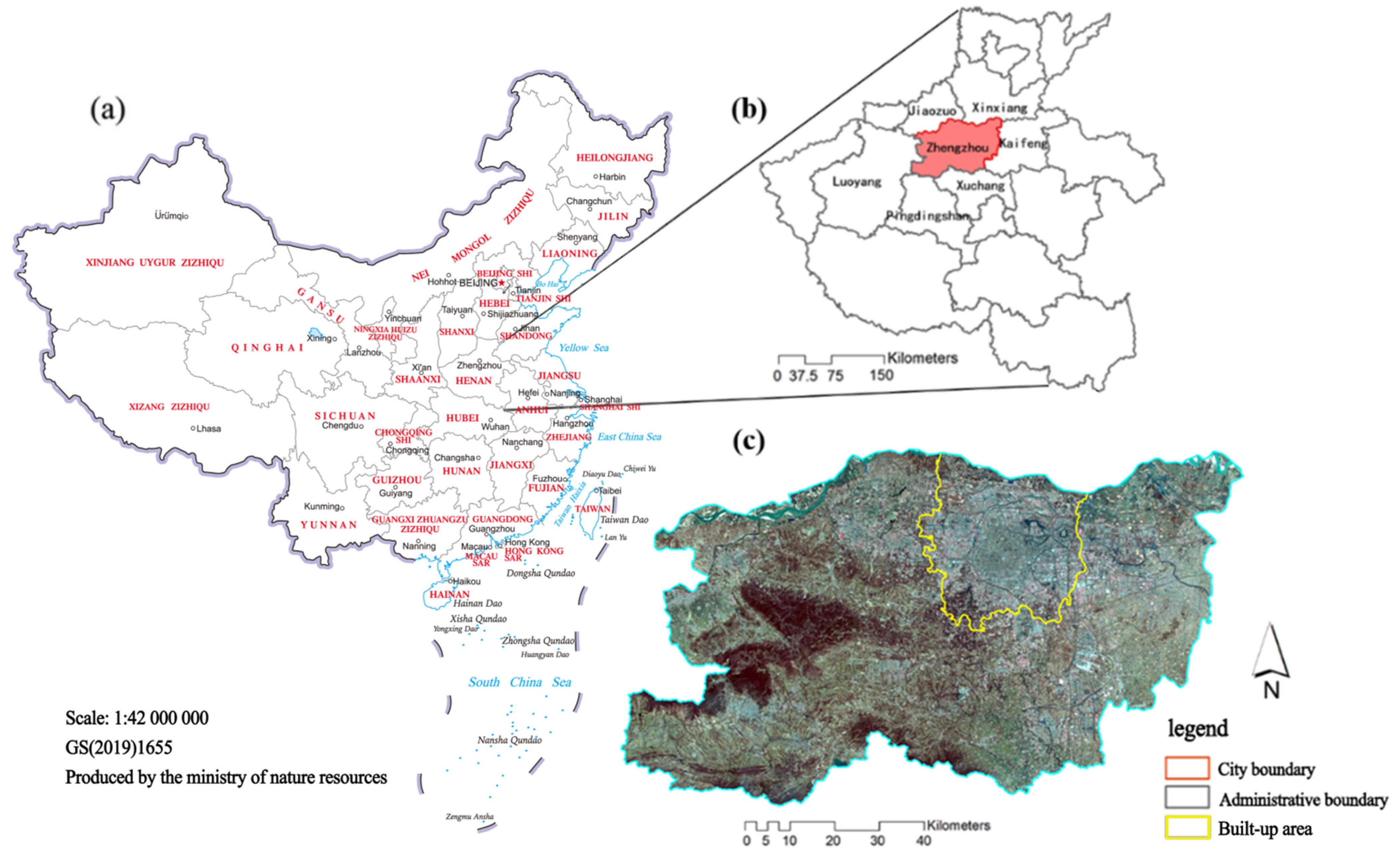
2.1. Study Area

Zhengzhou (34.7466° N, 113.6253° E) is the largest city of Henan province in China, with a total area of approximately 7446 km2. Its population has nearly doubled over the last 30 years, from approximately 5.6 million in 1990 to 10.4 million in 2019 [44]. In 2018, Henan ranked first in urbanization growth rate among Chinese provinces; thus Zhengzhou provides a typical example of rapid urbanization in central China. Zhengzhou is considered a “prefecture-level” city and thus includes substantial rural areas as well as urban built-up areas; it contains six municipal districts, five county-level cities, and one county (Figure 1). The urban built-up area is approximately 1181 km2 [45].
There are 124 rivers in Zhengzhou, with 29 large river basins belonging to the Yellow River or Huai River systems. The Yellow River system covers approximately one-quarter of the city’s total area and is the only perennial river in the area, while the Huai River system covers the remainder of the city. Two different water diversion projects have directly affected Zhengzhou’s waterbodies over the last 15 years: the South-to-North Water Diversion Project [46] and the Yellow River Diversion project [47]. The former project is the largest such project in Chinese history, and has the goal of transferring fresh water from southern China to northern China [48,49,50]. The latter project is much smaller in geographic scope and has the goal of drawing water from the Yellow River to enrich the Jialu River and Long Lake and Longzi Lake in Zhengzhou itself. Following these projects, in 2017, the government of Zhengzhou adopted the Wetland Protection Regulation, which required the forestry department to carry out a field survey of wetland resources. The survey mapped waterbodies and gathered ecological, geographical, ownership, management, and protection information for approximately 95% of waterbodies across the city. This manuscript is one outcome of that survey effort.

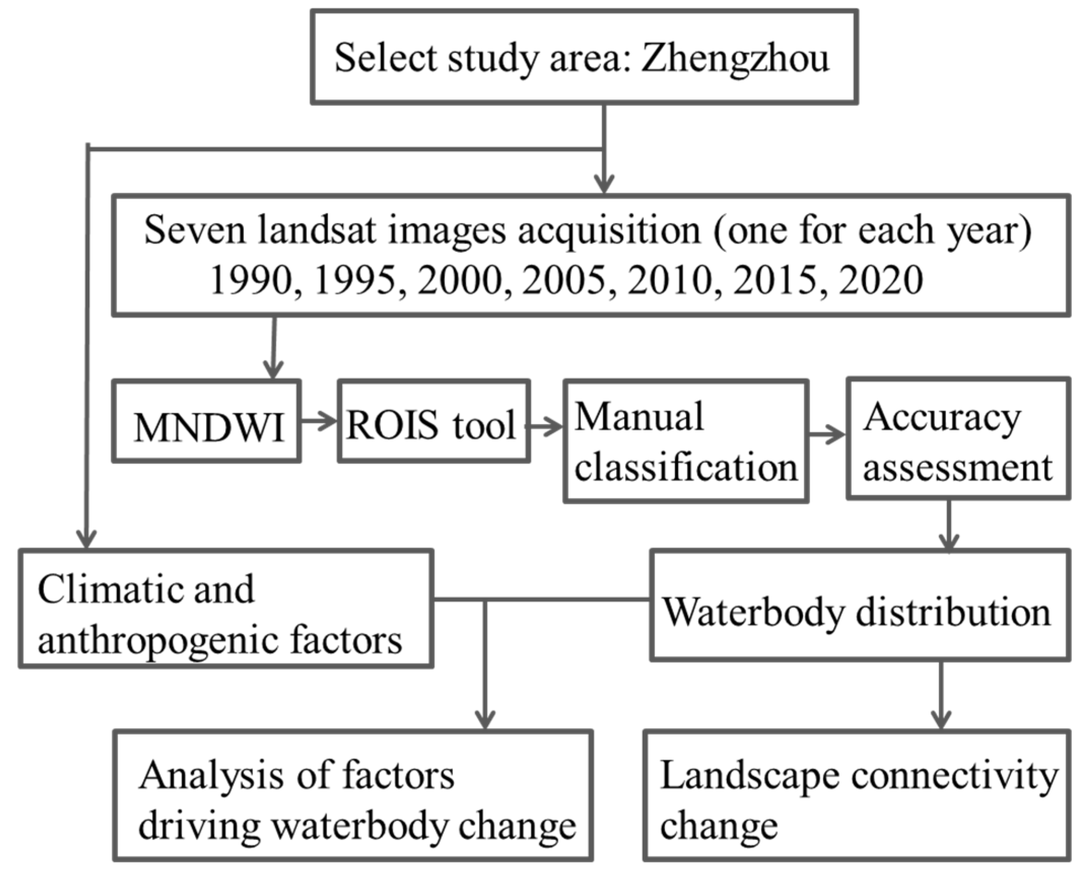
2.2. Satellite Image Acquisition and Processing

To evaluate the effect of urbanization on waterbodies in Zhengzhou, we observed changes in the landscape over the 30-year time period between 1990 and 2020. We chose 30 years as the study period because it covers the urbanization process of Zhengzhou, it is long enough to observe the effects of climate and anthropogenic factors on urban waterbodies, and data were available for this time period. We analyzed the landscape every 5 years during the 30-year period: in 1990, 1995, 2000, 2005, 2010, 2015, and 2020.
Seven Landsat satellite images were downloaded from EarthExplorer (USGS., https://earthexplorer.usgs.gov/, accessed on 20 July 2021), one for each year of the study (Figure 2). Landsat images have a 30 m resolution; this resolution imagery has been previously used for water identification [51,52,53]. Cloud-free images were selected from Landsat-5 TM (1990–2010), Landsat-7 ETM+ (2015), and Landsat-8 OLI/TIRS (2020), and reprojected into the World Geodetic System (WGS) 1984_UTM_49N coordinates. Each image was acquired in either May (2015, 2020) or June (1990–2010), to minimize the effects of seasonal variation in precipitation on the waterbody size [54]. Zhengzhou receives approximately 6 cm of precipitation in May and 9 cm in June [55,56].
In this paper, the Modified Normalized Difference Water Index (MNDWI) [53] was used to identify open water across Zhengzhou. MNDWI is similar to the Normalized Difference Water Index (NDWI) [57] but with the substitution of a middle-infrared (MIR) band, such as the Landsat TM band 5, which can be helpful in built-up and urban areas [53,58]. MNDWI uses the green and MIR bands to enhance open water features (Equation (1)). It also is sensitive to built-up features that are often correlated with open water in other indices.
MNDWI = (Green-MIR)/(Green + MIR)
Images were pre-processed using ENVI 5.3. We first calculated the MNDWI index, separated land and water using the band-of-interest thresholding tool, and performed a subset data extraction of water using the ROIS tool. All open water was then manually classified as one of the following seven waterbody types: perennial rivers, seasonal rivers and streams, lakes, canals, reservoirs, ponds, and aquaculture. Aquaculture sites were identified but excluded from further analysis because their value as bird habitats is hard to predict and can be negative [59,60], leaving six waterbody types in our analysis (Table 1). Manual classification relied largely on the map of wetland resources that was created during the aforementioned field survey of 2018; each identified waterbody was examined by eye, compared to the survey map, and then classified. When necessary, the classification and interpretation of waterbodies was also aided by information provided by the Zhengzhou Bureaus of Forestry and Water Resources.

2.3. Accuracy Assessment

We tested the accuracy of the open-water classification using stratified random sampling [61] with different waterbody types as the basis for stratification. We determined the sample size based on a 95% confidence level (α = 0.05) to create a confusion matrix [62,63]. We calculated the overall accuracy and kappa coefficient as well as the true positive rate (sensitivity) and the true negative rate (specificity) of each waterbody type. Gaofen-2 satellite images with 0.8 m resolution and timelapse imagery in Google Earth were the primary reference data sources.

2.4. Changes in Waterbody Distribution

To quantify the changes in waterbodies over time, we computed the following summary statistics for each type of waterbody in each 5-year period of the study: the total surface area of all waterbodies combined, maximum surface area of any individual waterbody, and total count of individual waterbodies. We focus our statistical analysis on total surface area but use the other summary statistics to provide additional insights about changes across the landscape. To test for significant changes in the total surface area of each waterbody type over time, we conducted a correlation analysis between the total surface area and time (i.e., year).

2.5. Potential Drivers of Waterbody Change

To evaluate potential drivers of waterbody change, we gathered a series of climate and anthropogenic variables that have been linked to waterbody changes in other studies: temperature [11], precipitation [64], potential evapotranspiration [65], human population density [66], the extent of built-up area [67], and the length of water-supply piping [68]. Each variable was measured repeatedly for each 5-year interval of the study.
Temperature and precipitation data for Zhengzhou were obtained from the China Meteorological Data Service Center (CMDC, https://data.cma.cn/en, accessed on 19 September 2021). These data included the average monthly temperature over the previous 12 months and average precipitation of the previous 6 and 12 months before the satellite image date. We calculated potential evapotranspiration using the SPEI package [69] in R [70]. The human population density, extent of built-up area, and length of water-supply piping in Zhengzhou were obtained from the Bureau of Statistics of Zhengzhou (http://tjj.zhengzhou.gov.cn/, accessed on 17 April 2021).

2.6. Linear Regression and Model Selection to Examine the Influence of Climatic and Anthropogenic Factors on Waterbody Change over Time

One priority of this study was to understand the drivers of waterbody change over time and, in particular, to contrast the relative importance of anthropogenic versus climatic drivers. However, several potential drivers were highly correlated over the time period (Table 2). The year was highly correlated (r > 0.95) with all anthropogenic variables and also significantly correlated with potential evapotranspiration and average monthly temperature. Given that the year is only a proxy for other changes within the city over time, it was excluded from further analyses. Correlations among anthropogenic variables were also extremely high (r > 0.96). Therefore, to avoid multicollinearity in our models, we removed the temperature and potential evapotranspiration as candidate variables and separated the remaining variables into two categories (climatic versus anthropogenic). Following this, climatic variables included six- and twelve-month precipitation, and anthropogenic variables included built-up area, length of water supply piping, and population density. There were no significant correlations between the remaining variables in different groups (Table 2).
Linear modeling was used to assess the drivers of waterbody change from 1990 to 2020. Each waterbody type was considered independently, with the total surface area of each waterbody type in each 5-year interval as the response variable. Predictor variables included the climatic and anthropogenic variables described above, each measured in 1990, 1995, 2000, 2005, 2015, and 2020. To ensure that highly correlated variables were excluded from the same model and to keep the number of predictor variables sufficiently low for our small sample size, we first included only one climatic or anthropogenic variable in each model. The best-supported variable for each category was determined using the Corrected Akaike Information Criterion (AICc) [71] to compare linear models with single predictor variables. Finally, the two best-supported (and uncorrelated) predictor variables were combined into a single linear model for each waterbody type. Statistical analyses were performed in RStudio.

2.7. Evaluating Landscape Connectivity

To evaluate changes in aquatic habitat connectivity over time, we used Conefor 2.6 [72]. Conefor is a frequently used software package for evaluating landscape- and patch-level connectivity in a variety of habitats and landscapes [73,74,75]. In our analyses, individual waterbodies were considered ‘patches’ and connections between patches were considered from the perspective of waterfowl (i.e., family Anatidae). Among waterfowl, one of the most well-studied species is the mallard (Anas platyrhynchos), a duck with generalist feeding habits that breeds in a wide variety of habitats and has broad distribution around the world [76,77,78,79]. This species has been shown to use small urban waterbodies [80] and was observed at many Zhengzhou waterbodies during the wetland resource survey described above; thus we used published mallard-related data to parameterize our connectivity models. Research has shown that the mallard’s average flight distance is 0.4 km [81], so we assumed that many ducks would travel this distance in a single flight event.
We used the waterbody maps created for each time period (1990, 1995, 2000, 2005, 2010, 2015, 2020), along with the Conefor ArcGIS extension, to create the ‘node’ (i.e., patch) and ‘connection’ input files for Conefor 2.6. Each year was analyzed separately. In Conefor, we set the connectivity distance to 0.4 km and the probability value to 0.5. We used the probability of connectivity index (PC) [82] to analyze the landscape- and patch-level connectivity changes over time for waterfowl in Zhengzhou. PC represents the probability that two randomly placed points within the landscape are accessible from each other (i.e., interconnected), and is calculated as follows in Equation (2):
PC = i = 1 n j = 1 n a i × a j × p i j * A L 2 = PC n u m A L 2
where a i and a j are the area (or other attributes) of patches i and j , p ij is the probability of direct movement between patches i and j , and A L represents the total landscape area, including habitat and non-habitat patches. PC ranges from 0 to 1; when PC equals 0, there are no habitat patches in the landscape, and when the entire landscape is covered by habitat, the PC value is equal to 1.
PC is a landscape-level attribute, but the proportion of connectivity attributed to each patch can be calculated by removing that patch and recalculating the landscape attribute, as shown in Equation (3) [83]:
dPC k = 100 × PC PC r e m o v e , k PC = 100 × Δ PC k PC
The resulting change in PC(dPC) measures the importance of that patch to landscape connectivity. dPC can be further divided into three parts according to a patch’s contribution to different aspects of connectivity. dPCintra measures within-patch connectivity and is a function of available habitat within the patch. dPCflux measures the area-weighted dispersal flux through a patch. Finally, dPCconnector measures the degree to which a patch connects other patches on the landscape [84].
We first examined PC in each 5-year interval to look for landscape-scale changes in connectivity over time. We subsequently examined differences in dPC among waterbody types to see if certain types of waterbodies contributed more or less to landscape-scale connectivity. The Yellow River was excluded from the dPC analyses because its large surface area and spread from east to west Zhengzhou caused it to dominate all indices and obscured changes in the other waterbody types.
As the data were not normally distributed, we used Kruskal–Wallis [85] and Dunn’s post hoc tests [86] to examine the differences in dPC values between different waterbody categories in each study year, with significance based on Bonferroni corrections. Non-parametric statistics and visualization were performed in RStudio, and we used ArcGIS 10.2.2 to map the dPC of each waterbody in each study period. Finally, for each study year, we extracted the top 100 waterbodies with respect to each aspect of connectivity (dPCintra, dPCflux, and dPCconnector) in a separate analysis of waterbody connectivity over time.

3. Results

3.1. Waterbody Classification Accuracy

The overall classification accuracy ranged from 87% to 96%, and the final kappa coefficients for the classification scheme ranged from 0.83 to 0.94 (Table 3). Cohen [87] suggested that kappa values between 0.80 and 0.90 be interpreted as ‘strong’ and values above 0.90 as almost perfect agreement, so our classification scheme performed very well based on these results. Sensitivity and specificity are shown in Appendix A.

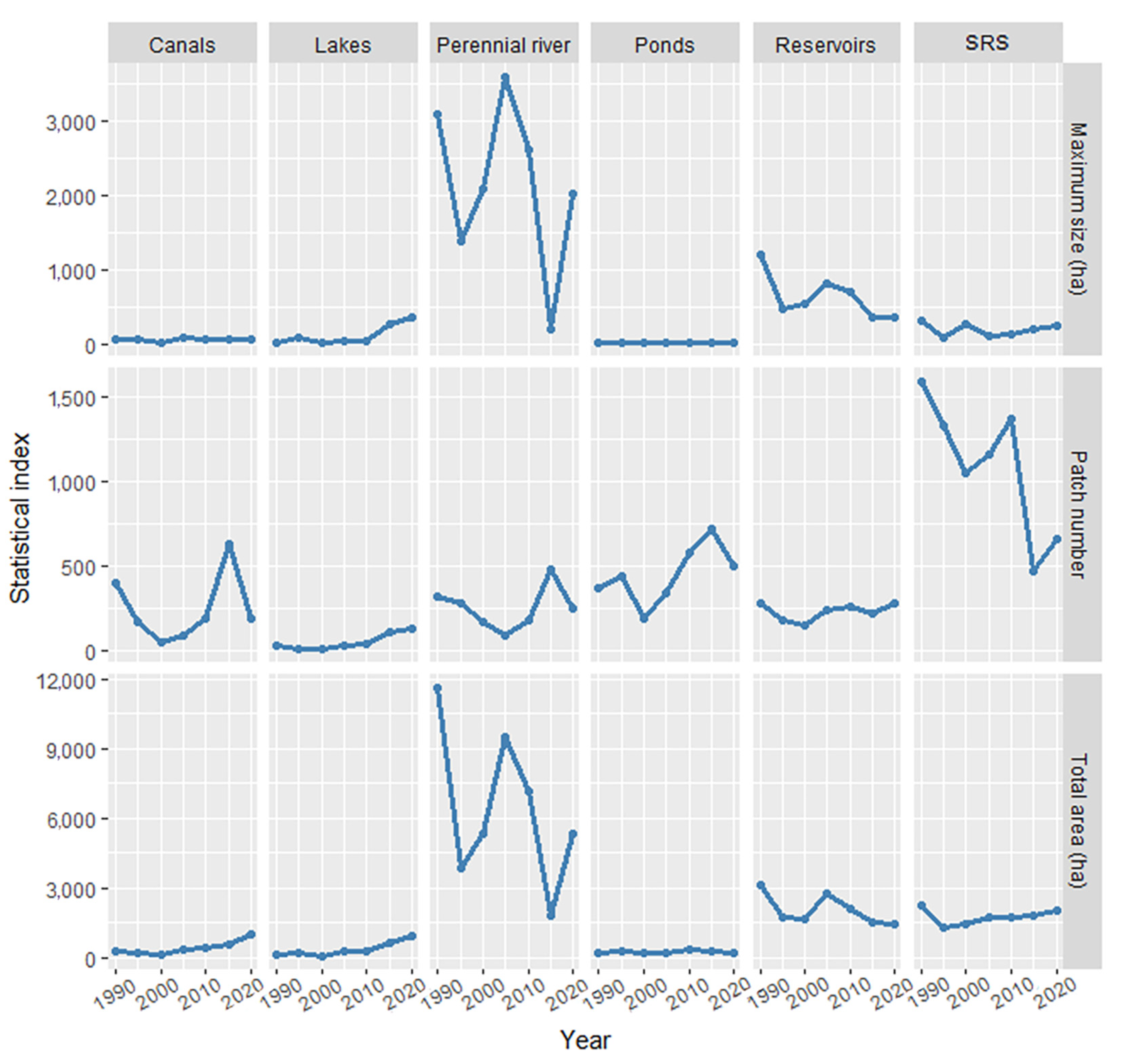
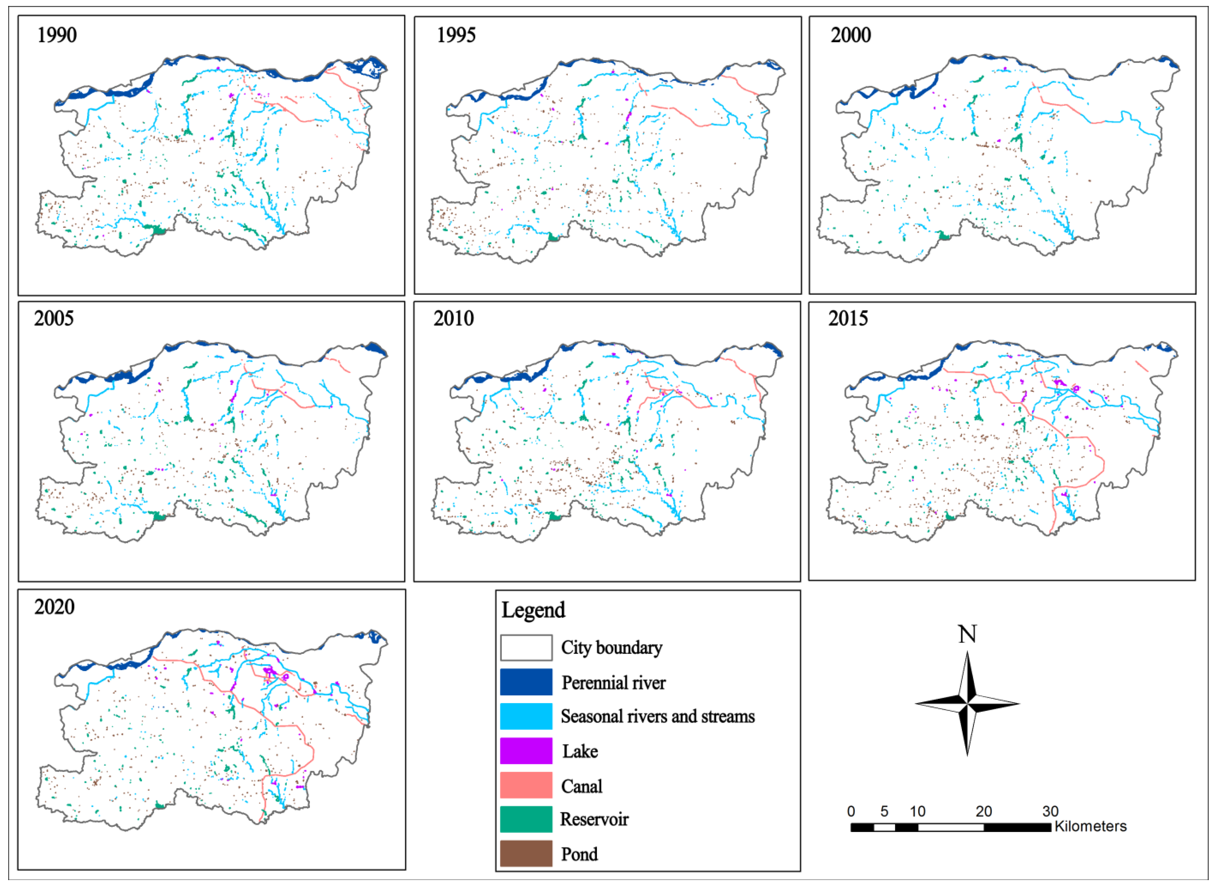
3.2. Waterbody Dynamic Changes

From 1990 to 2020, the number, size, and total surface area of different kinds of waterbodies changed substantially (Figure 3 and Figure 4). The only statistically significant changes were seen in the total surface area of lakes and canals, both of which increased over time (lakes: r = 0.87, p = 0.01; canals: r = 0.82, p = 0.02). The total surface area of lakes increased from 116 hectares in 1990 to 942 hectares in 2020, an increase of 712%. This change was clearly due to the increase in number of lakes and the addition of large lakes (Figure 3). The total surface area of canals increased 236% over the same time period, from 310 to 1042 hectares. The perennial river and the reservoirs both fluctuated in surface area over time, with peaks in the first year of the study and again in 2005. Ponds and seasonal rivers and streams showed relatively little change over the study period (Figure 3).

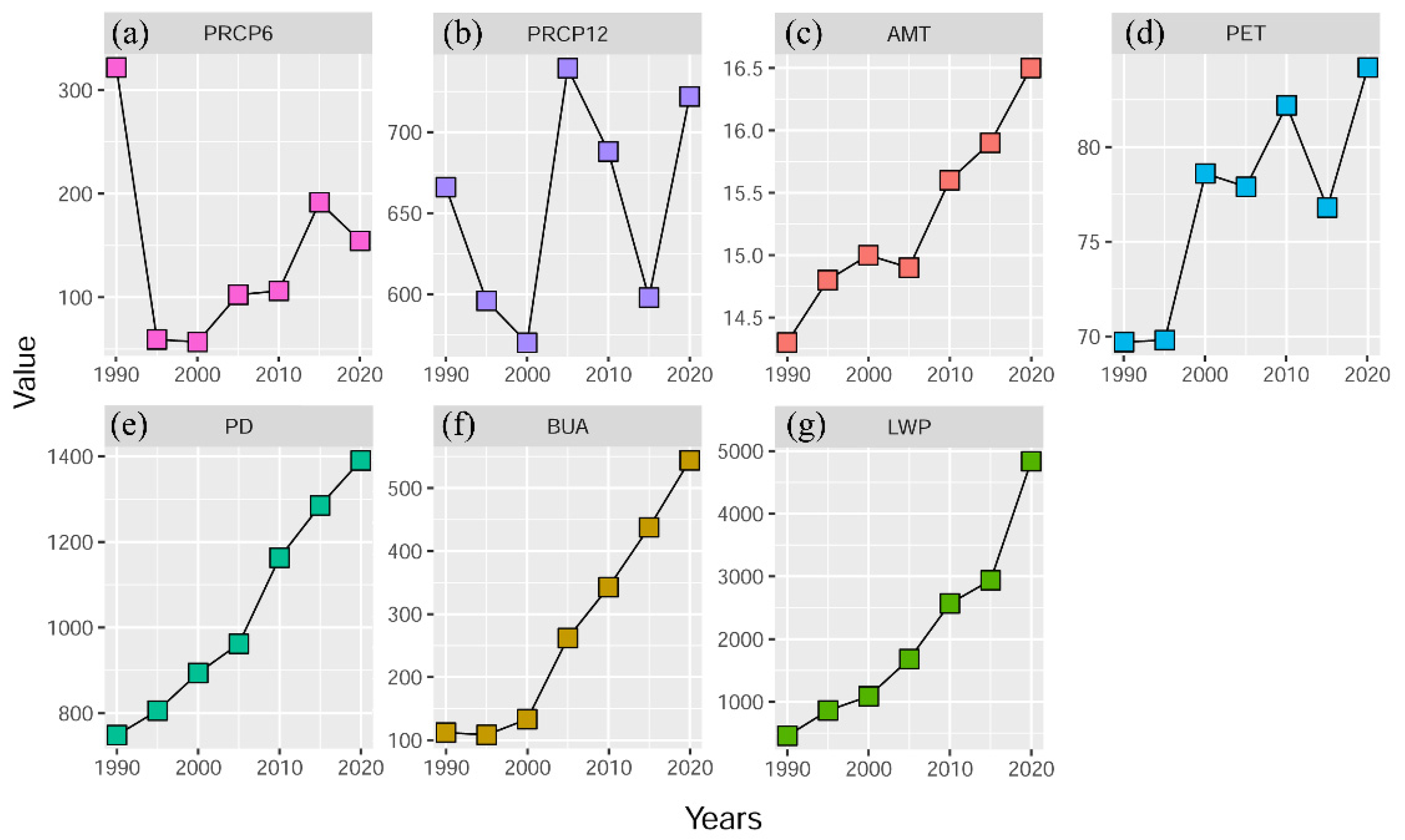
3.3. Driving Factors of Urban Waterbody Change

Over the 30-year study period, the total population of Zhengzhou increased almost linearly from 5.578 million to 10 million people and the built-up area and length of water pipeline followed a similar trend (Figure 5). These land-use change patterns are likely responsible for the observed concurrent increase in annual mean temperature and potential evapotranspiration (Figure 5). Precipitation fluctuated over the study period, with the 6-month precipitation highest in the first year of the study and the 12-month precipitation highest in 2005.
Among the climatic variables, six-month precipitation was the best predictor of the surface area of the perennial river, seasonal rivers and streams, and reservoirs (Table 4). Twelve-month precipitation was the best predictor of the surface area of lakes, canals, and ponds. However, there was little difference in AICc between the two precipitation variables for most waterbodies. Among the anthropogenic variables, population density was best supported for the perennial river, reservoirs, and ponds; extent of built-up area was selected for seasonal rivers and streams; and the length of water pipeline was the best supported for lakes and canals (Table 4).
Table 4. Selection of the most predictive climatic and anthropogenic variables for the total surface area of each waterbody type. Corrected Akaike Information Criterion (AICc) values are shown in the table and were used to select the predictor variables for the linear regression models shown in Table 5. The variables of AICc from low to high are indicated by ① ② ③.
WaterbodyClimatic Anthropogenic
6-Month Precipitation12-Month PrecipitationPopulation DensityBuilt-Up AreaLength of Water Pipeline
Perennial river140.3892 ①141.5736 ②142.8388 ①143.4732 ③143.0368 ②
Seasonal rivers and streams103.0762 ①110.3008 ②112.5721 ③111.8918 ①112.3397 ②
Lakes113.1882 ②112.4519 ①101.7744 ③99.1148 ②97.6410 ①
Canals112.6251 ②111.0877 ①103.6491 ③100.1516 ②98.4526 ①
Reservoirs121.6092 ①122.2174 ②120.8713 ①122.0940 ③121.3000 ②
Ponds89.1690 ②88.8273 ①88.7068 ①88.8032 ②88.9787 ③
After identifying the best climatic and anthropogenic drivers for each type of waterbody, we combined them into a single linear regression model to explain the total surface area of each waterbody type. Models for the seasonal rivers and streams, lakes, and canals had high explanatory power (adjusted r2 > 0.83), with the anthropogenic variable having a significant positive effect on the total surface area of lakes and canals and precipitation having a significant positive effect on the surface area of seasonal rivers and streams. Regression models for the perennial river, reservoirs, and ponds did not have high explanatory power or any significant variables.
Table 5. Linear regression for the total surface area of each type of waterbody (waterbody~ climatic variables + anthropogenic variables). Significant variables are highlighted with bold text. PRCP6 represents average monthly precipitation in the 6 months prior to satellite image capture; PRCP12 represents average monthly precipitation in the 12 months prior to satellite image capture; PD represents population density; BUA represents built-up area; LWP represents length of water pipeline.
WaterbodyClimateAnthropogenic
VariableCoefficientp-ValueVariableCoefficientp-ValueAdjusted R2 of Full Model
Perennial riverPRCP618.84200.1410PD−4.22700.33800.3106
Seasonal rivers and streamsPRCP62.85640.0066BUA0.64920.09510.8381
LakesPRCP12−0.35560.6902LWP0.20220.00520.8466
CanalsPRCP120.59550.5213LWP0.18020.00850.8352
ReservoirsPRCP63.58160.1920PD−1.53760.15000.3909
PondsPRCP120.13520.7640PD0.04770.6980−0.3652

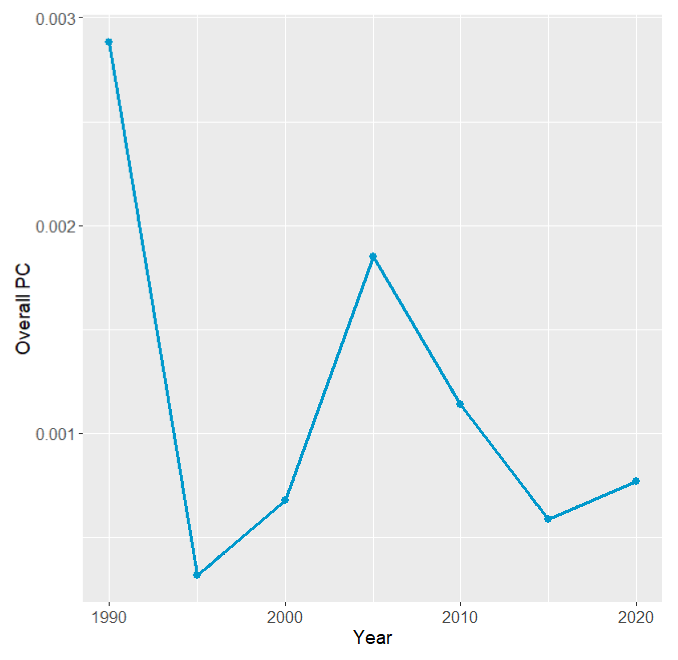
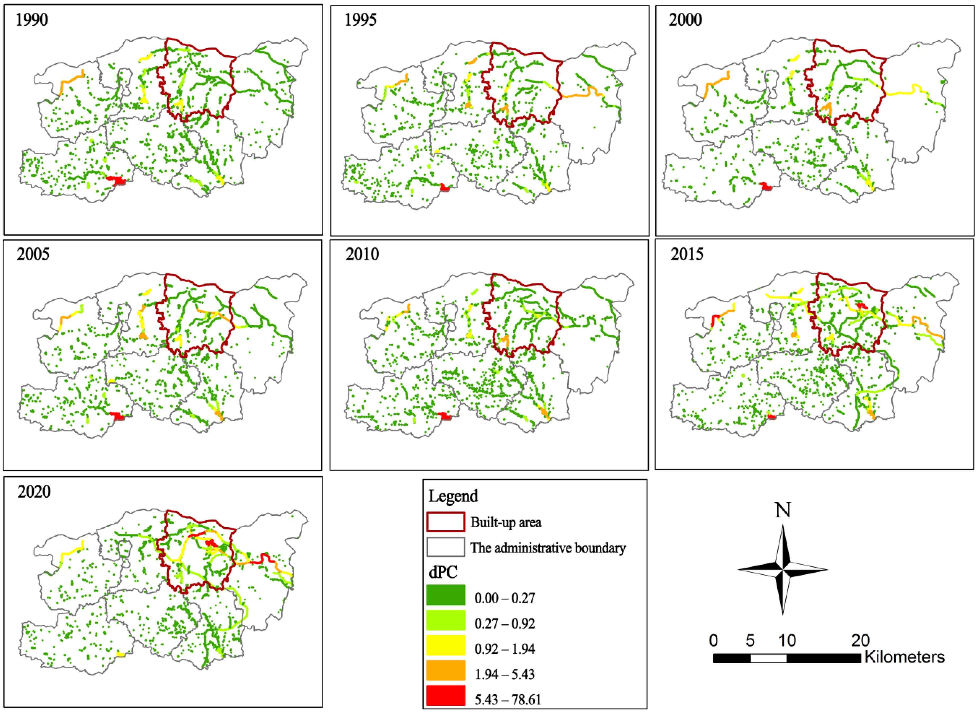
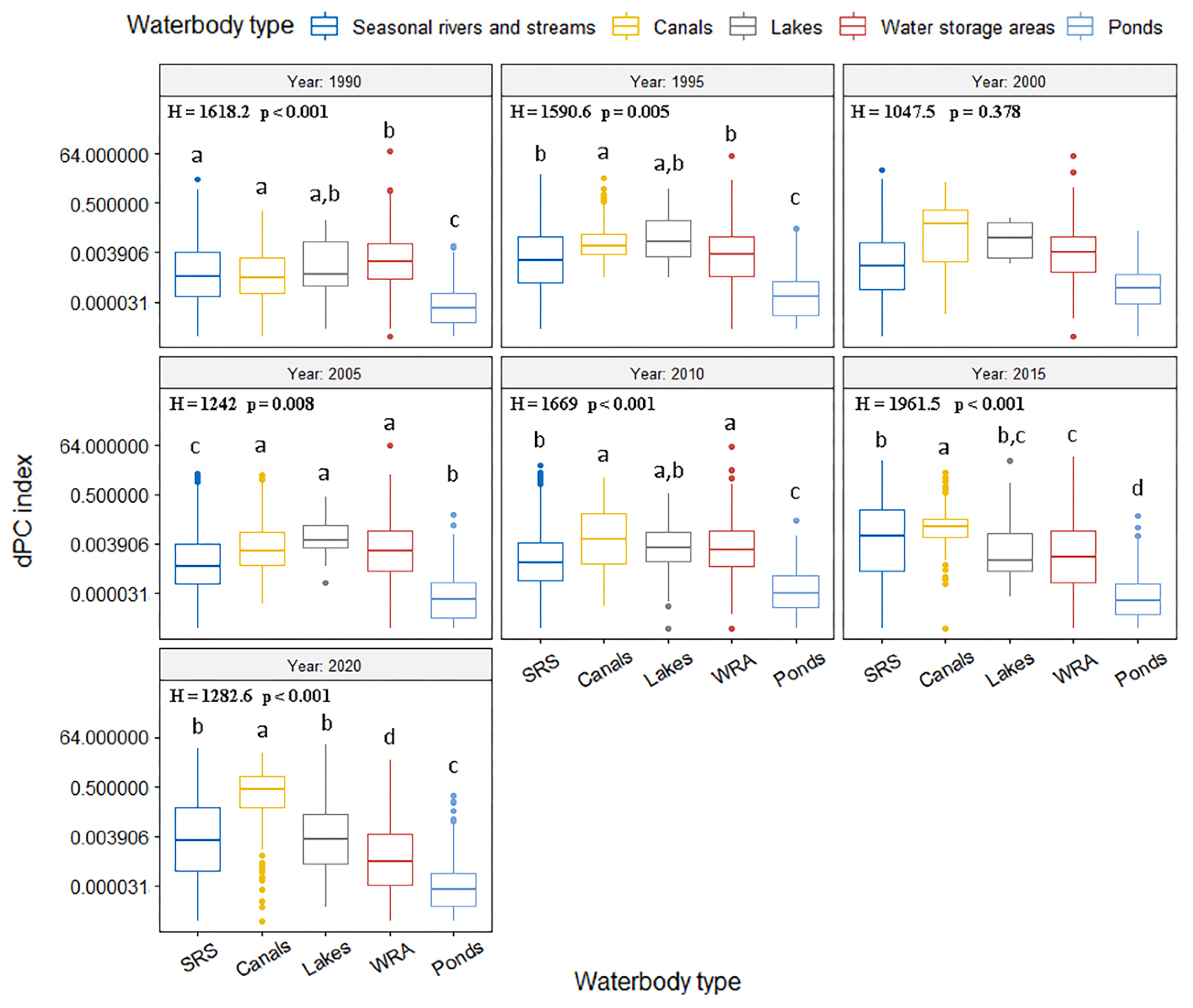
3.4. Landscape Connectivity Analysis

While the PC did not consistently decrease over time, the connectivity was greatest at the beginning of the study period in 1990 (Figure 6). The connectivity briefly increased in 2005 before dropping off again but was still approximately 36% less than the PC value in 1990 (Figure 6).
In comparing the contribution of individual waterbodies to overall landscape connectivity, we see significant differences between waterbody types in every year except 2000 (p < 0.001 for Kruskal–Wallis tests, Figure 7, Appendix B). Ponds have significantly lower dPC than other waterbody types most years of the study. Reservoirs and lakes have the highest dPC in early years of the study, but canals have the highest dPC in later years. By 2020, the main urban area of Zhengzhou appears to contain the waterbodies with the highest contribution to connectivity within the city (Figure 8).
Our analysis of the top 100 waterbodies that contribute most to landscape connectivity each year showed that seasonal rivers and streams are very important for all aspects of connectivity (Table 6). However, their importance seemed to diminish over time. Reservoirs were also quite important for dPCintra and, to a lesser degree, dPC flux. Canals increased in importance over time for all aspects of connectivity but seemed to play the largest role in dPCconnector.

4. Discussion

Our study illustrates substantial changes in the surface water distribution and connectivity in Zhengzhou over a 30-year timespan, which were driven by both climatic and anthropogenic factors. These results highlight the high spatiotemporal variability that can characterize freshwater aquatic systems. This kind of variability has been seen in other Chinese cities [88,89] and in a rapidly urbanizing region in southwest Australia [90] over similar time periods. We found statistically significant increases in the total surface area of lakes and canals over time, while the area of reservoirs and the perennial river fluctuated but showed a non-significant decreasing trend from 1990 to 2020. The increase in area of lakes was accompanied by an increase in number of lakes and size of the largest lake, as several new lakes were created in the built-up areas of the city over the last two decades (Figure 4). Canals were also created as part of the two water diversion projects in Zhengzhou. The wetland resource surveys commissioned by the Zhengzhou government as well as some local news reports [91,92] show that these constructed waterbodies are used by many wildlife species, including waterfowl. This use by wildlife suggests that their construction could potentially offset other negative effects of urbanization. However, the increase in waterbody area we observed in the urban core is not the norm in most cities. For example, a study of 32 other major Chinese cities found that the total surface area of urban lakes decreased by 24% from 1990 to 2015 [93]. Therefore, we want to caution that urbanization in general is unlikely to have net positive effects on waterfowl or other wildlife.
We found that the length of water pipe was correlated with an increase in surface area of lakes and canals, and precipitation correlated with an increase in surface area of seasonal rivers and streams. Liu et al. (2020) [94] also found that anthropogenic variables had a stronger effect on lakes than natural variables, but they mainly found a negative effect on lake area change. This disparity may be explained by the fact that Liu et al. (2020) focused on natural lakes, whereas our “lake” category included constructed lakes as well. We likely see a positive effect of anthropogenic variables on the lake and canal area because they are correlated with human construction of these waterbody types. Seasonal rivers and streams, however, are highly dependent on precipitation for recharge [95], which may explain why climatic variables played a stronger role in determining the change in their surface area. The Yellow River Diversion Project has been drawing water from the Yellow River since 2009 [96], so we might expect to see decreases in the surface area of the Yellow River associated with anthropogenic variables. However, none of our predictor variables were significantly related to area of the Yellow River. On visual inspection, the fluctuations of the Yellow River resemble a superimposition of the 6-month and 12-month precipitation patterns, so it may be that we did not measure precipitation at the most relevant time scale for the Yellow River. It is also likely that the area of the Yellow River will decline over time due to the continued diversion of water.
The overall landscape connectivity, as measured by the PC index, fluctuated in Zhengzhou over time. The temporal pattern in connectivity appears similar to the pattern for the total surface area of the perennial river. The perennial river, i.e., the Yellow River, contains the majority of the water in Zhengzhou and spans the entire city from east to west. For this reason, the perennial river plays a dominant role in the overall connectivity of aquatic habitats. If the area of the Yellow River does decline over time in the future, as we speculated above, then that could have long-term and large-scale impacts on landscape connectivity. However, other kinds of waterbodies also contribute to landscape connectivity. Seasonal rivers and streams, for example, play an important role in connecting other waterbodies and supporting flux of waterfowl across the landscape, as seen by their high values of dPCflux and dPCconnector. This is likely because their linear form gives them proximity to many other waterbodies. Interestingly, we noticed increased connectivity values of waterbodies in the main urban district over time. This finding is counter to an analysis of 100 cities in the United States of America, in which the connectivity of waterbodies was found to decrease in the most urbanized areas [15].
Many of the changes we observed in Zhengzhou seem to be unique among urban areas. Some of these changes—in particular, the addition of artificial waterbodies and associated increase in connectivity in the most urban parts of Zhengzhou—can be attributed to specific local and regional planning and policies. For example, in 2000, an old military airport was removed from Zhengzhou and the municipal government proposed a new town in its place. A plan was developed by a Japanese architect that involved the creation of several new waterbodies in what is now the main urban area [97]. One of the new lakes became the waterbody with the greatest overall contribution to landscape connectivity in the region (Figure 8). Other changes in the landscape, particularly the canals, are attributed to the subsequent regional hydraulic projects [49]. As development in Zhengzhou was specifically planned to include open water, the patterns we detected in this system may be different from those seen in cities that did not intentionally include open water in their design.
Although the importance of wetlands has been recognized for many decades [98], urban wetlands have been relatively neglected compared to more natural habitats. Previous urban water system planning has been largely focused on meeting hydrological functions such as water supply and flood control [99,100], and most studies on waterbird protection have focused on areas such as nature reserves, coastal wetland landscapes [101], or more rural landscapes [102]. One exception is a study of Beijing, China, that examined habitat suitability and connectivity for the mallard duck (along with two other bird species; [80]), although only a single time period was examined. Our paper provides a novel contribution by exploring urban waterbird protection from the perspective of changes in the connectivity of urban water bodies over time. We hope to provide a new perspective on regional water system planning and waterbird conservation in urbanized areas and suggest that the overall landscape connectivity of the entire city or even region should be considered during planning. Water management strategies that disproportionately focus on certain areas within a landscape but ignore others can be problematic for migratory or otherwise highly mobile organisms such as waterbirds that require resources from multiple spatially distinct waterbodies [103]. The conservation or construction of waterbodies outside of the main urban areas may help contribute to a robust network of aquatic habitats region-wide, which may in turn help to increase the resilience of waterbird populations in the face of a changing climate [104].
Our results show both increases and decreases in aquatic habitat and connectivity over time, with changes driven by both anthropogenic and climatic factors. While we believe these results reflect real changes happening in Zhengzhou, they should be considered in light of some limitations of this study. In particular, we used only seven time periods for our analysis. A longer temporal extent might reveal when key changes in aquatic habitat began, and more frequent sampling periods could potentially reveal stronger relationships with climatic drivers. Moreover, the use of satellite imagery with higher spatial resolution could prove useful for monitoring smaller waterbodies and subtle shoreline changes in larger waterbodies. Future studies could also validate the classification of key waterbodies by using high-resolution GNSS receivers as well as more automated classification methods. Additional studies could consider the impacts of redistributing water resources at a larger scale (e.g., across the entire country) and how best to maintain and improve urban surface-water landscape connectivity. It would also be interesting to conduct a more qualitative analysis of the many complex social factors that affect land use and land cover change over time, as our variables did not explain the changes in all waterbody types. Finally, we suggest that future research could validate our connectivity analyses with fieldwork (e.g., placing GPS trackers on mallards) and expand the focus to other waterfowl or other taxa that use urban waterbodies. The work presented here is a first step toward understanding changes in aquatic habitats in Zhengzhou and we hope that it can assist in informing future urban planning strategies that benefit both people and wildlife.

5. Conclusions

Aquatic habitat availability and connectivity are critical to maintaining biodiversity and ecosystem services in urban landscapes. However, these aquatic habitats are often threatened by the process of urbanization. An in-depth analysis of the changes in aquatic habitats and their underlying drivers can help planners to propose efficient and targeted conservation and planning strategies. Using remotely sensed images from 1990 to 2020, we studied the spatial distribution, connectivity, and changes of urban waterbodies in a rapidly urbanizing area of central China. We found evidence of substantial changes in surface water distribution and connectivity in Zhengzhou over 30 years, driven by both climate and anthropogenic changes. Some categories of waterbodies significantly increased in surface area, while others fluctuated over time but showed decreasing trends. These changes in waterbody area caused fluctuations in landscape connectivity and, unintuitively, an apparent increase in connectivity in the urban built-up area. These results show that urbanization can have unexpected and potentially positive effects on the connectivity of surface water, although these results might not translate directly to positive effects on wildlife.

Author Contributions

Conceptualization, C.L. and G.T.; methodology, E.S.M.; software, M.B.G.; validation, E.S.M., C.L. and M.B.G.; formal analysis, C.L., E.S.M. and M.B.G.; investigation, C.L. and B.M.; resources, B.M.; data curation, C.L.; writing—original draft preparation, C.L.; writing—review and editing, E.S.M. and M.B.G.; visualization, C.L.; supervision, E.S.M.; project administration, G.T.; funding acquisition, G.T. All authors have read and agreed to the published version of the manuscript.

Funding

This research was funded by Urban–Rural Green Space Resources Control and Landscape Ecological Design Disciplinary Innovation and Talents Introduction Centre Program (GXJD006), National Natural Science Foundation of China (51808198).

Data Availability Statement

The data presented in this study are available on request from the first author.

Acknowledgments

We would like to thank the Zhengzhou Forestry Bureau for their strong support during the survey and data collection phase, and for the supporting documents issued when entering some private or prohibited territories for the survey. We also thank the Zhengzhou Water Resources Department for providing relevant basic information.

Conflicts of Interest

The authors declare no conflict of interest.

Appendix A

Supporting Information Table 3. Sensitivity and specificity table.
Table A1. Sensitivity and specificity for the classification of each waterbody type in each year of the study.
1990Overall Accuracy
93%
Kappa Coefficient
0.91
SensitivitySpecificity
Perennial river11
Seasonal rivers and streams0.880.99
Lakes11
Canals0.881
Aquaculture0.880.99
Reservoirs10.99
Ponds0.810.99
Non-water0.990.94
1995Overall Accuracy
92%
Kappa Coefficient
0.89
SensitivitySpecificity
Perennial river0.890.99
Seasonal rivers and streams0.891
Lakes11
Canals11
Aquaculture0.900.99
Reservoirs11
Ponds0.880.97
Non-water0.970.96
2000Overall Accuracy
93%
Kappa Coefficient
0.90
SensitivitySpecificity
Perennial river10.99
Seasonal rivers and streams0.831
Lakes11
Canals10.99
Aquaculture0.940.98
Reservoirs0.751
Ponds0.780.99
Non-water0.960.94
2005Overall Accuracy
95%
Kappa Coefficient
0.93
SensitivitySpecificity
Perennial river11
Seasonal rivers and streams0.970.99
Lakes11
Canals10.99
Aquaculture0.961
Reservoirs11
Ponds0.701
Non-water0.980.96
2010Overall Accuracy
87%
Kappa Coefficient
0.83
SensitivitySpecificity
Perennial river0.941
Seasonal rivers and streams0.820.99
Lakes11
Canals11
Aquaculture0.921
Reservoirs0.941
Ponds0.610.98
Non-water0.980.89
2015Overall Accuracy
89%
Kappa Coefficient
0.84
SensitivitySpecificity
Perennial river10.99
Seasonal rivers and streams0.841
Lakes11
Canals11
Aquaculture0.950.99
Reservoirs0.941
Ponds0.551
Non-water0.960.88
2020Overall Accuracy
96%
Kappa Coefficient
0.94
SensitivitySpecificity
Perennial river11
Seasonal rivers and streams11
Lakes11
Canals11
Aquaculture0.971
Reservoirs11
Ponds0.641
Non-water0.980.96

Appendix B

Supporting Information Figure 7. Dunn’s post hoc tests comparing dPC of different types of waterbodies.
Table A2. 1990 Dunn’s post hoc tests, with p-values adjusted with the Bonferroni method.
Col Mean-
Row Mean
CanalsLakesPondsSeasonal Rivers and Streams
Lakes−1.262379
1.0000
Ponds14.82517
0.0000 *
7.054761
0.0000 *
Seasonal rivers and streams−0.749351
1.0000
1.064317
1.0000
−19.22657
0.0000 *
Reservoirs−5.826354
0.0000 *
−1.194882
1.0000
−19.16881
0.0000 *
−6.344683
0.0000 *
* represents that the p value is less than 0.05, and there is a difference between the two groups of data.
Table A3. 1995 Dunn’s post hoc tests, with p-values adjusted with the Bonferroni method.
Col Mean-
Row Mean
CanalsLakesPondsSeasonal Rivers and Stream
Lakes−0.330870
1.0000
Ponds18.76464
0.0000 *
6.741065
0.0000 *
Seasonal rivers and streams6.937147
0.0000 *
2.496341
0.1255
−20.39078
0.0000 *
Reservoirs4.355784
0.0001 *
2.046934
0.4066
−13.89612
0.0000 *
−1.252919
1.0000
* represents that the p value is less than 0.05, and there is a difference between the two groups of data.
Table A4. 2005 Dunn’s post hoc tests, with p-values adjusted with the Bonferroni method.
Col Mean-
Row Mean
CanalsLakesPondsSeasonal Rivers and Streams
Lakes−2.086112
0.3697
Ponds12.82851
0.0000 *
10.43303
0.0000 *
Seasonal rivers and streams4.110059
0.0004 *
4.857113
0.0000 *
−17.03069
0.0000 *
Reservoirs0.207174
1.0000
2.404186
0.1621
−17.40335
0.0000 *
−5.842903
0.0000 *
* represents that the p value is less than 0.05, and there is a difference between the two groups of data.
Table A5. 2010 Dunn’s post hoc tests, with p-values adjusted with the Bonferroni method.
Col Mean-
Row Mean
CanalsLakesPondsSeasonal Rivers and Streams
Lakes1.412300
1.0000
Ponds18.85677
0.0000 *
8.808351
0.0000 *
Seasonal rivers and streams7.886307
0.0000 *
2.541924
0.1102
−19.58719
0.0000 *
Reservoirs2.450383
0.1427
0.059137
1.0000
−17.09649
0.0000 *
−5.174021
0.0000 *
* represents that the p value is less than 0.05, and there is a difference between the two groups of data.
Table A6. 2015 Dunn’s post hoc tests, with p-values adjusted with the Bonferroni method.
Col Mean-
Row Mean
CanalsLakesPondsSeasonal Rivers and Streams
Lakes6.283624
0.0000 *
Ponds32.62254
0.0000 *
11.17535
0.0000 *
Seasonal rivers and streams6.196535
0.0000 *
−2.552837
0.1068
−23.74914
0.0000 *
Reservoirs9.667919
0.0000 *
0.920139
1.0000
−13.46839
0.0000 *
4.629104
0.0000 *
* represents that the p value is less than 0.05, and there is a difference between the two groups of data.
Table A7. 2020 Dunn’s post hoc tests, with p-values adjusted with the Bonferroni method.
Col Mean-
Row Mean
CanalsLakesPondsSeasonal Rivers and Streams
Lakes6.366440
0.0000 *
Ponds23.98440
0.0000 *
13.40196
0.0000 *
Seasonal streams10.33210
0.0000 *
1.313172
0.1068
−20.19719
0.0000 *
Reservoirs13.48855
0.0000 *
5.094971
0.0000 *
−10.51564
0.0000 *
5.836825
0.0000 *
* represents that the p value is less than 0.05, and there is a difference between the two groups of data.

References

  1. Mitsch, W.J.; Bernal, B.; Nahlik, A.; Mander, Ü.; Zhang, L.; Anderson, C.J.; Jørgensen, S.E.; Brix, H. Wetlands, carbon, and climate change. Landsc. Ecol. 2013, 28, 583–597. [Google Scholar] [CrossRef]
  2. Mitsch, W.J.; Gosselink, J.G. The value of wetlands: Importance of scale and landscape setting. Ecol. Econ. 2000, 35, 25–33. [Google Scholar] [CrossRef]
  3. Park, C.Y.; Lee, D.K.; Asawa, T.; Murakami, A.; Kim, H.G.; Lee, M.K.; Lee, H.S. Influence of urban form on the cooling effect of a small urban river. Landsc. Urban Plan. 2019, 183, 26–35. [Google Scholar] [CrossRef]
  4. Ehrenfeld, J.G. Evaluating wetlands within an urban context. Urban Ecosyst. 2000, 4, 69–85. [Google Scholar] [CrossRef]
  5. Ma, C.; Zhang, G.; Zhang, X.; Zhao, Y.; Li, H. Application of Markov model in wetland change dynamics in Tianjin Coastal Area, China. Procedia Environ. Sci. 2012, 13, 252–262. [Google Scholar] [CrossRef] [Green Version]
  6. Gibbs, J.P. Wetland Loss and Biodiversity Conservation. Conserv. Biol. 2000, 14, 314–317. [Google Scholar] [CrossRef] [Green Version]
  7. Holland, C.C.; Honea, J.; Gwin, S.E.; Kentula, M.E. Wetland degradation and loss in the rapidly urbanizing area of Portland, Oregon. Wetlands 1995, 15, 336–345. [Google Scholar] [CrossRef]
  8. Cai, Y.; Zhang, H.; Pan, W.; Chen, Y.; Wang, X. Urban expansion and its influencing factors in Natural Wetland Distribution Area in Fuzhou City, China. Chin. Geogr. Sci. 2012, 22, 568–577. [Google Scholar] [CrossRef]
  9. YangFan, L.; YaLou, S.; XiaoDong, Z.; HuHua, C.; Tao, Y. Coastal Wetland Loss and Environmental Change Due to Rapid Urban Expansion in Lianyungang, Jiangsu, China. Reg. Environ. Chang. 2014, 14, 1175–1188. [Google Scholar]
  10. Davidson, N.C. How much wetland has the world lost? Long-term and recent trends in global wetland area. Mar. Freshw. Res. 2014, 65, 934–941. [Google Scholar] [CrossRef]
  11. Xi, Y.; Peng, S.; Ciais, P.; Chen, Y. Future impacts of climate change on inland Ramsar wetlands. Nat. Clim. Chang. 2021, 11, 45–51. [Google Scholar] [CrossRef]
  12. Xu, H.; Lin, D.; Tang, F. The impact of impervious surface development on land surface temperature in a subtropical city: Xiamen, China. Int. J. Clim. 2013, 33, 1873–1883. [Google Scholar] [CrossRef]
  13. Ali, A.K.M.; Al Ramahi, F.K.M. A study of the Effect of Urbanization on Annual Evaporation Rates in Baghdad City Using Remote Sensing. Iraqi J. Sci. 2020, 61, 2142–2149. [Google Scholar] [CrossRef]
  14. Kaufmann, R.K.; Seto, K.C.; Schneider, A.; Liu, Z.; Zhou, L.; Wang, W. Climate Response to Rapid Urban Growth: Evidence of a Human-Induced Precipitation Deficit. J. Clim. 2007, 20, 2299–2306. [Google Scholar] [CrossRef]
  15. Steele, M.K.; Heffernan, J. Morphological characteristics of urban water bodies: Mechanisms of change and implications for ecosystem function. Ecol. Appl. 2014, 24, 1070–1084. [Google Scholar] [CrossRef]
  16. Misra, A.K. Impact of Urbanization on the Hydrology of Ganga Basin (India). Water Resour. Manag. 2011, 25, 705–719. [Google Scholar] [CrossRef]
  17. Zhou, H.; Shi, P.; Wang, J.; Yu, D.; Gao, L. Rapid Urbanization and Implications for River Ecological Services Restoration: Case Study in Shenzhen, China. J. Urban Plan. Dev. 2011, 137, 121–132. [Google Scholar] [CrossRef]
  18. Verheijen, B.H.F.; Varner, D.M.; Haukos, D.A. Effects of large-scale wetland loss on network connectivity of the Rainwater Basin, Nebraska. Landsc. Ecol. 2018, 33, 1939–1951. [Google Scholar] [CrossRef] [Green Version]
  19. Heintzman, L.J.; McIntyre, N.E. Quantifying the effects of projected urban growth on connectivity among wetlands in the Great Plains (USA). Landsc. Urban Plan. 2019, 186, 1–12. [Google Scholar] [CrossRef]
  20. Ren, W.; Zhong, Y.; Meligrana, J.; Anderson, B.; Watt, W.; Chen, J.; Leung, H.-L. Urbanization, land use, and water quality in Shanghai: 1947–1996. Environ. Int. 2003, 29, 649–659. [Google Scholar] [CrossRef]
  21. Sievers, M.; Hale, R.; Parris, K.; Swearer, S. Impacts of human-induced environmental change in wetlands on aquatic animals. Biol. Rev. 2018, 93, 529–554. [Google Scholar] [CrossRef] [PubMed] [Green Version]
  22. McIntyre, N.; Wright, C.K.; Swain, S.; Hayhoe, K.; Liu, G.; Schwartz, F.W.; Henebry, G. Climate forcing of wetland landscape connectivity in the Great Plains. Front. Ecol. Environ. 2014, 12, 59–64. [Google Scholar] [CrossRef]
  23. Franczyk, J.; Chang, H. The effects of climate change and urbanization on the runoff of the Rock Creek basin in the Portland metropolitan area, Oregon, USA. Hydrol. Process. 2009, 23, 805–815. [Google Scholar] [CrossRef]
  24. Ogden, J.C. Nesting by Wood Storks in Natural, Altered, and Artificial Wetlands in Central and Northern Florida. Colon. Waterbirds 1991, 14, 39. [Google Scholar] [CrossRef]
  25. Ma, Z.; Li, B.; Zhao, B.; Jing, K.; Tang, S.; Chen, J. Are artificial wetlands good alternatives to natural wetlands for waterbirds? A case study on Chongming Island, China. Biodivers. Conserv. 2004, 13, 333–350. [Google Scholar] [CrossRef]
  26. Xu, X.; Xie, Y.; Qi, K.; Luo, Z.; Wang, X. Detecting the Response of Bird Communities and Biodiversity to Habitat Loss and Fragmentation Due to Urbanization. Sci. Total Environ. 2018, 624, 1561–1576. [Google Scholar] [CrossRef]
  27. Ward, M.P.; Semel, B.; Herkert, J.R. Identifying the ecological causes of long-term declines of wetland-dependent birds in an urbanizing landscape. Biodivers. Conserv. 2010, 19, 3287–3300. [Google Scholar] [CrossRef]
  28. Li, D.; Chen, S.; Lloyd, H.; Zhu, S.; Shan, K.; Zhang, Z. The importance of artificial habitats to migratory waterbirds within a natural/artificial wetland mosaic, Yellow River Delta, China. Bird Conserv. Int. 2013, 23, 184–198. [Google Scholar] [CrossRef] [Green Version]
  29. Giosa, E.; Mammides, C.; Zotos, S. The importance of artificial wetlands for birds: A case study from Cyprus. PLoS ONE 2018, 13, e0197286. [Google Scholar] [CrossRef]
  30. Xia, S.; Liu, Y.; Wang, Y.; Chen, B.; Jia, Y.; Liu, G.; Yu, X.; Wen, L. Wintering waterbirds in a large river floodplain: Hydrological connectivity is the key for reconciling development and conservation. Sci. Total Environ. 2016, 573, 645–660. [Google Scholar] [CrossRef]
  31. Maltby, E. Wetland management goals: Wise use and conservation. Landsc. Urban Plan. 1991, 20, 9–18. [Google Scholar] [CrossRef]
  32. Verhoeven, J.T.A.; Arheimer, B.; Yin, C.; Hefting, M. Regional and global concerns over wetlands and water quality. Trends Ecol. Evol. 2006, 21, 96–103. [Google Scholar] [CrossRef]
  33. Amezaga, J.; Santamaria, L.; Green, A.J. Biotic wetland connectivity—Supporting a new approach for wetland policy. Acta Oecol. 2002, 23, 213–222. [Google Scholar] [CrossRef] [Green Version]
  34. Wiegleb, G.; Dahms, H.U.; Byeon, W.I.; GyeWoon, C. To What Extent Can Constructed Wetlands Enhance Biodi-versity? Int. J. Environ. Sci. Dev. 2017, 8, 561–569. [Google Scholar] [CrossRef] [Green Version]
  35. Rudnick, D.; Ryan, S.; Beier, P.; Cushman, S.; Dieffenbach, F.; Epps, C.; Gerber, L.; Hartter, J.; Jenness, J.; Kintsch, J.; et al. The Role of Landscape Connectivity in Planning and Implementing Conservation and Restoration Priorities. Issues Ecol. 2012, 16, 1–20. [Google Scholar]
  36. Li, G.; Sun, S.; Fang, C. The varying driving forces of urban expansion in China: Insights from a spatial-temporal analysis. Landsc. Urban Plan. 2018, 174, 63–77. [Google Scholar] [CrossRef]
  37. Fang, C.L.; Li, G.D.; Zhang, Q. The Variation Characteristics and Control Measures of theUrban Construction Land in China. J. Nat. Res. 2017, 32, 363–376. [Google Scholar] [CrossRef]
  38. Mao, D.; Wang, Z.; Wu, J.; Wu, B.; Zeng, Y.; Song, K.; Yi, K.; Luo, L. China’s wetlands loss to urban expansion. Land Degrad. Dev. 2018, 29, 2644–2657. [Google Scholar] [CrossRef]
  39. Xu, W.; Fan, X.; Ma, J.; Pimm, S.L.; Kong, L.; Zeng, Y.; Li, X.; Xiao, Y.; Zheng, H.; Liu, J.; et al. Hidden Loss of Wetlands in China. Curr. Biol. 2019, 29, 3065–3071.e2. [Google Scholar] [CrossRef] [Green Version]
  40. Ma, T.; Sun, S.; Fu, G.; Hall, J.W.; Ni, Y.; He, L.; Yi, J.; Zhao, N.; Du, Y.; Pei, T.; et al. Pollution exacerbates China’s water scarcity and its regional inequality. Nat. Commun. 2020, 11, 650. [Google Scholar] [CrossRef] [Green Version]
  41. Yang, S.-Q.; Liu, P.-W. Strategy of water pollution prevention in Taihu Lake and its effects analysis. J. Great Lakes Res. 2010, 36, 150–158. [Google Scholar] [CrossRef] [Green Version]
  42. Guo, Z.; Liu, W.; Zhang, M.; Zhang, Y.; Li, X. Transforming the wetland conservation system in China. Mar. Freshw. Res. 2020, 71, 1469. [Google Scholar] [CrossRef]
  43. Xu, H.; Wang, S.; Xue, D. Biodiversity conservation in China: Legislation, Plans and Measures. Biodivers. Conserv. 1999, 8, 819–837. [Google Scholar] [CrossRef]
  44. Population by Year—Zhengzhou Bureau of Statistics. Available online: http://tjj.zhengzhou.gov.cn/ndsj/3134558.jhtml (accessed on 17 April 2021).
  45. Policy Interpretation of the Notice of the People’s Government of Zhengzhou City on the Size of the Built-up Area of Zhengzhou City in 2019—Zhengzhou Municipal Government. Available online: http://public.zhengzhou.gov.cn/interpretdepart/3550365.jhtml (accessed on 17 April 2021).
  46. Liu, C.; Zheng, H. South-to-north Water Transfer Schemes for China. Int. J. Water Resour. Dev. 2002, 18, 453–471. [Google Scholar] [CrossRef]
  47. Drabarek, A. Control and Management of Yellow River Diversion Project Conveyance Line. In Hydroinformatics; World Scientific: Singapore, 2004; pp. 1915–1922. [Google Scholar]
  48. Zheng, J.; Ge, Q.; Li, M.; Zhang, X.; Liu, H.; Hao, Z. Drought/flood spatial patterns in centennial cold and warm periods of the past 2000 years over eastern China. Chin. Sci. Bull. 2014, 59, 2964–2971. [Google Scholar] [CrossRef]
  49. Cai, X. Water stress, water transfer and social equity in Northern China—Implications for policy reforms. J. Environ. Manag. 2008, 87, 14–25. [Google Scholar] [CrossRef] [PubMed]
  50. Liu, J.; Zang, C.; Tian, S.; Liu, J.; Yang, H.; Jia, S.; You, L.; Liu, B.; Zhang, M. Water conservancy projects in China: Achievements, challenges and way forward. Glob. Environ. Chang. 2013, 23, 633–643. [Google Scholar] [CrossRef] [Green Version]
  51. Liu, Z.; Yao, Z.; Wang, R. Assessing methods of identifying open water bodies using Landsat 8 OLI imagery. Environ. Earth Sci. 2016, 75, 1–13. [Google Scholar] [CrossRef]
  52. Xu, D.; Zhang, D.; Shi, D.; Luan, Z. Automatic Extraction of Open Water Using Imagery of Landsat Series. Water 2020, 12, 1928. [Google Scholar] [CrossRef]
  53. Xu, H. Modification of normalised difference water index (NDWI) to enhance open water features in remotely sensed imagery. Int. J. Remote. Sens. 2006, 27, 3025–3033. [Google Scholar] [CrossRef]
  54. Mu, B.; Mayer, A.L.; He, R.; Tian, G. Land use dynamics and policy implications in Central China: A case study of Zhengzhou. Cities 2016, 58, 39–49. [Google Scholar] [CrossRef]
  55. Zhengzhou Climate: Average Temperature, Weather by Month, Zhengzhou Weather Averages—Climate-Data.Org. Available online: https://en.climate-data.org/asia/china/henan/zhengzhou-2731/ (accessed on 19 September 2021).
  56. CMDC. Available online: https://data.cma.cn/en (accessed on 19 September 2021).
  57. Gao, B.-C. NDWI—A normalized difference water index for remote sensing of vegetation liquid water from space. Remote Sens. Environ. 1996, 58, 257–266. [Google Scholar] [CrossRef]
  58. Szabó, S.; Gácsi, Z.; Balázs, B. Specific Features of NDVI, NDWI and MNDWI as Reflected in Land Cover Categories. Landsc. Environ. 2016, 10, 194–202. [Google Scholar] [CrossRef]
  59. Barrett, L.T.; Swearer, S.; Dempster, T. Impacts of marine and freshwater aquaculture on wildlife: A global meta-analysis. Rev. Aquac. 2019, 11, 1022–1044. [Google Scholar] [CrossRef]
  60. Bechard, M.; Márquez-Reyes, C. Mortality of Wintering Ospreys and Other Birds at Aquaculture Facilities in Colombia. J. Raptor Res. 2003, 37, 292–298. [Google Scholar]
  61. Stehman, S.V. Estimating the Kappa Coefficient and Its Variance under Stratified Random Sampling. Photogramm. Eng. Remote Sens. 1996, 62, 401–407. [Google Scholar]
  62. Congalton, R.G.; Green, K. Assessing the Accuracy of Remotely Sensed Data: Principles and Practices, 3rd ed.; CRC Press: Boca Raton, FL, USA, 2019; ISBN 978-0-429-62935-8. [Google Scholar]
  63. Congalton, R.G. A review of assessing the accuracy of classifications of remotely sensed data. Remote Sens. Environ. 1991, 37, 35–46. [Google Scholar] [CrossRef]
  64. Rooney, G.G.; Van Lipzig, N.; Thiery, W. Estimating the effect of rainfall on the surface temperature of a tropical lake. Hydrol. Earth Syst. Sci. 2018, 22, 6357–6369. [Google Scholar] [CrossRef] [Green Version]
  65. Balling, R.C.; Brazel, S.W. The impact of rapid urbanization on pan evaporation in phoenix. Arizona. J. Clim. 1987, 7, 593–597. [Google Scholar] [CrossRef]
  66. Wu, J.; Stewart, T.W.; Thompson, J.R.; Kolka, R.K.; Franz, K. Watershed features and stream water quality: Gaining insight through path analysis in a Midwest urban landscape, USA. Landsc. Urban Plan. 2015, 143, 219–229. [Google Scholar] [CrossRef] [Green Version]
  67. Assen, M. Land Use/Cover Dynamics and Its Implications in the Dried Lake Alemaya Watershed, Eastern Ethiopia. J. Sustain. Dev. Afr. 2011, 13, 267–284. [Google Scholar]
  68. Ayeni, A. Increasing Population, Urbanization and Climatic Factors in Lagos State, Nigeria: The Nexus and Implications on Water Demand and Supply. J. Glob. Initiat. Policy Pedagog. Perspect. 2017, 11, 69–87. [Google Scholar]
  69. Vicente-Serrano, S.M.; Beguería, S.; López-Moreno, J.I. A Multiscalar Drought Index Sensitive to Global Warming: The Standardized Precipitation Evapotranspiration Index. J. Clim. 2010, 23, 1696–1718. [Google Scholar] [CrossRef] [Green Version]
  70. R Core Team. R: A Language and Environment for Statistical Computing; R Foundation for Statistical Computing: Vienna, Austria, 2019. [Google Scholar]
  71. Hurvich, C.M.; Tsai, C.-L. A Corrected Akaike Information Criterion for Vector Autoregressive Model Selection. J. Time Ser. Anal. 1993, 14, 271–279. [Google Scholar] [CrossRef]
  72. Saura, S.; Torné, J. Conefor Sensinode 2.2: A software package for quantifying the importance of habitat patches for landscape connectivity. Environ. Model. Softw. 2009, 24, 135–139. [Google Scholar] [CrossRef]
  73. Engelhard, S.L.; Huijbers, C.M.; Stewart-Koster, B.; Olds, A.D.; Schlacher, T.A.; Connolly, R.M. Prioritising seascape connectivity in conservation using network analysis. J. Appl. Ecol. 2017, 54, 1130–1141. [Google Scholar] [CrossRef] [Green Version]
  74. Ramirez-Reyes, C.; Bateman, B.; Radeloff, V.C. Effects of habitat suitability and minimum patch size thresholds on the assessment of landscape connectivity for jaguars in the Sierra Gorda, Mexico. Biol. Conserv. 2016, 204, 296–305. [Google Scholar] [CrossRef]
  75. Flantua, S.G.; O’Dea, A.; Onstein, R.E.; Giraldo, C.; Hooghiemstra, H. The flickering connectivity system of the north Andean páramos. J. Biogeogr. 2019, 46, 1808–1825. [Google Scholar] [CrossRef]
  76. Johnsgard, P.A. Evolutionary Relationships among the North American Mallards. Auk 1961, 78, 3–43. [Google Scholar] [CrossRef] [Green Version]
  77. Maak, S.; Wimmers, K.; Weigend, S.; Neumann, K. Isolation and characterization of 18 microsatellites in the Peking duck (Anas platyrhynchos) and their application in other waterfowl species. Mol. Ecol. Notes 2003, 3, 224–227. [Google Scholar] [CrossRef]
  78. Baratti, M.; Cordaro, M.; Dessì-Fulgheri, F.; Vannini, M.; Fratini, S. Molecular and ecological characterization of urban populations of the mallard (Anas platyrhynchos L.) in Italy. Ital. J. Zool. 2009, 76, 330–339. [Google Scholar] [CrossRef]
  79. Bengtsson, D.; Avril, A.; Gunnarsson, G.; Elmberg, J.; Söderquist, P.; Norevik, G.; Tolf, C.; Safi, K.; Fiedler, W.; Wikelski, M.; et al. Movements, Home-Range Size and Habitat Selection of Mallards during Autumn Migration. PLoS ONE 2014, 9, e100764. [Google Scholar] [CrossRef] [Green Version]
  80. Lv, Z.; Yang, J.; Wielstra, B.; Wei, J.; Xu, F.; Si, Y. Prioritizing Green Spaces for Biodiversity Conservation in Beijing Based on Habitat Network Connectivity. Sustainability 2019, 11, 2042. [Google Scholar] [CrossRef] [Green Version]
  81. Kleyheeg, E.; Van Dijk, J.G.B.; Tsopoglou-Gkina, D.; Woud, T.Y.; Boonstra, D.K.; Nolet, B.; Soons, M. Movement patterns of a keystone waterbird species are highly predictable from landscape configuration. Mov. Ecol. 2017, 5, 1–14. [Google Scholar] [CrossRef] [PubMed] [Green Version]
  82. Saura, S.; Pascual-Hortal, L. A new habitat availability index to integrate connectivity in landscape conservation planning: Comparison with existing indices and application to a case study. Landsc. Urban Plan. 2007, 83, 91–103. [Google Scholar] [CrossRef]
  83. Urban, D.; Keitt, T. Landscape Connectivity: A Graph-Theoretic Perspective. Ecology 2001, 82, 1205–1218. [Google Scholar] [CrossRef]
  84. Saura, S.; Rubio, L. A common currency for the different ways in which patches and links can contribute to habitat availability and connectivity in the landscape. Ecography 2010, 33, 523–537. [Google Scholar] [CrossRef]
  85. Choi, W.; Lee, J.W.; Huh, M.-H.; Kang, S.-H. An Algorithm for Computing the Exact Distribution of the Kruskal–Wallis Test. Commun. Stat. Simul. Comput. 2003, 32, 1029–1040. [Google Scholar] [CrossRef]
  86. Dinno, A. Nonparametric Pairwise Multiple Comparisons in Independent Groups using Dunn’s Test. Stata J. Promot. Commun. Stat. Stata 2015, 15, 292–300. [Google Scholar] [CrossRef] [Green Version]
  87. McHugh, M.L. Interrater reliability: The kappa statistic. Biochem. Med. 2012, 22, 276–282. [Google Scholar] [CrossRef]
  88. Deng, X.; Xu, Y.; Han, L.; Song, S.; Yang, L.; Li, G.; Wang, Y. Impacts of Urbanization on River Systems in the Taihu Region, China. Water 2015, 7, 1340–1358. [Google Scholar] [CrossRef]
  89. Wu, L.; Xu, Y.; Yuan, J.; Xu, Y.; Wang, Q.; Xu, X.; Wen, H. Impacts of Land Use Change on River Systems for a River Network Plain. Water 2018, 10, 609. [Google Scholar] [CrossRef] [Green Version]
  90. Tulbure, M.G.; Kininmonth, S.; Broich, M. Spatiotemporal dynamics of surface water networks across a global biodiversity hotspot—Implications for conservation. Environ. Res. Lett. 2014, 9, 114012. [Google Scholar] [CrossRef]
  91. Henan Daily News-Swan Frequently Appear in Zhengzhou Dragon Lake. Available online: https://www.henandaily.cn/content/szheng/rdyw/2016/0314/2089.html (accessed on 6 September 2021).
  92. Ruddy Shelduck, the Most Beautiful Scenery of Dongfeng Canal. Available online: https://www.163.com/dy/article/GE1FC8MF05450U67.html (accessed on 6 September 2021).
  93. Xie, C.; Huang, X.; Wang, L.; Fang, X.; Liao, W. Spatiotemporal change patterns of urban lakes in China’s major cities between 1990 and 2015. Int. J. Digit. Earth 2017, 11, 1085–1102. [Google Scholar] [CrossRef]
  94. Liu, X.; Shi, Z.; Huang, G.; Bo, Y.; Chen, G. Time Series Remote Sensing Data-Based Identification of the Dominant Factor for Inland Lake Surface Area Change: Anthropogenic Activities or Natural Events? Remote Sens. 2020, 12, 612. [Google Scholar] [CrossRef] [Green Version]
  95. Jennings, D.B.; Jarnagin, S.T. Changes in Anthropogenic Impervious Surfaces, Precipitation and Daily Streamflow Discharge: A Historical Perspective in a Mid-Atlantic Subwatershed. Landsc. Ecol. 2002, 17, 471–489. [Google Scholar] [CrossRef]
  96. Eco-Water System Overview—Zhengzhou Water Resources Bureau. Available online: http://zzsl.zhengzhou.gov.cn/stsx/2735866.jhtml (accessed on 17 April 2021).
  97. Xue, Q.C.; Wang, Y.; Tsai, L. Building new towns in China—A case study of Zhengdong New District. Cities 2013, 30, 223–232. [Google Scholar] [CrossRef]
  98. Gardner, R.C.; Davidson, N.C. The Ramsar Convention. In Wetlands: Integrating Multidisciplinary Concepts; LePage, B.A., Ed.; Springer Netherlands: Dordrecht, The Netherlands, 2011; pp. 189–203. ISBN 978-94-007-0551-7. [Google Scholar]
  99. Garen, D.C. Revised Surface-Water Supply Index for Western United States. J. Water Resour. Plan. Manag. 1993, 119, 437–454. [Google Scholar] [CrossRef]
  100. Morita, M. Quantification of increased flood risk due to global climate change for urban river management planning. Water Sci. Technol. 2011, 63, 2967–2974. [Google Scholar] [CrossRef] [PubMed]
  101. Li, D.; Chen, S.; Guan, L.; Lloyd, H.; Liu, Y.; Lv, J.; Zhang, Z. Patterns of waterbird community composition across a natural and restored wetland landscape mosaic, Yellow River Delta, China. Estuarine Coast. Shelf Sci. 2011, 91, 325–332. [Google Scholar] [CrossRef]
  102. Naugle, D.E.; Johnson, R.R.; Estey, M.E.; Higgins, K.F. A landscape approach to conserving wetland bird habitat in the prairie pothole region of eastern South Dakota. Wetlands 2001, 21, 1–17. [Google Scholar] [CrossRef]
  103. Haig, S.M.; Mehlman, D.W.; Oring, L.W. Avian Movements and Wetland Connectivity in Landscape Conservation. Conserv. Biol. 2008, 12, 749–758. [Google Scholar] [CrossRef]
  104. Reese, G.C.; Skagen, S.K. Modeling nonbreeding distributions of shorebirds and waterfowl in response to climate change. Ecol. Evol. 2017, 7, 1497–1513. [Google Scholar] [CrossRef] [PubMed]
Figure 1. (a) Location of Zhengzhou, Henan Province, in China; gray lines indicate the boundaries of provinces and territories. (b) Henan province; black lines depict city boundaries. (c) Satellite image of Zhengzhou; the area within the yellow polygon is the built-up area of Zhengzhou.
Land 10 01070 g001
Figure 2. Workflow steps in our analysis.
Land 10 01070 g002
Figure 3. Spatiotemporal distribution of waterbodies in Zhengzhou from 1990 to 2020. (top row) The size of the largest individual waterbody in each category; (middle row) the number of waterbodies in each category; (bottom row) the total surface area of all waterbodies each category. SRS is an abbreviation for seasonal rivers and streams.
Land 10 01070 g003
Figure 4. The distribution of urban waterbodies in Zhengzhou from 1990 to 2020. Note the additions in 2015 of two large lakes in the northeast of the city and the canal that runs from northwest to southeast.
Land 10 01070 g004
Figure 5. Potential driving factors influencing changes in surface water from 1990 to 2020 in Zhengzhou, China. (a) Average monthly precipitation in the 6 months prior to satellite image capture (PRCP6, mm), (b) average monthly precipitation in the 12 months prior to satellite image capture (PRCP12, mm), (c) annual mean temperature (AMT, °C), (d) potential evapotranspiration (PET, mm), (e) population density (PD, human population per km2), (f) built-up area (BUA, km2), and (g) length of water pipeline (LWP, km).
Land 10 01070 g005
Figure 6. Overall connectivity of urban waterbodies from 1990 to 2020, as measured by the PC index.
Land 10 01070 g006
Figure 7. The contribution of individual waterbodies to overall landscape connectivity, as measured by the dPC index. For each study year from 1990 to 2020, we compared dPC between different kinds of wetlands using Kruskal–Wallis and Dunn’s tests. Test details are in Appendix B. Statistical significance was based on Bonferroni corrections. Kruskal–Wallis test statistics are shown in the plot for each year. Pairwise comparisons (a–d) are notated for significance (p < 0.05) for Dunn’s tests. SRS indicate seasonal rivers and streams. The perennial river was excluded from analysis since it dominated all connectivity measures.
Land 10 01070 g007
Figure 8. Variation in dPC over a 30-year period in Zhengzhou, China. The index was divided into five categories by the Jenks natural breaks classification method. The perennial river was excluded from the analysis to better understand the changes in connectivity of the other waterbody types in Zhengzhou.
Land 10 01070 g008
Table 1. Six classes of open waterbodies analyzed in this study.
Waterbody TypePreviewDescription
Perennial river Land 10 01070 i001A stream or river (channel) that has continuous flow in parts of its stream bed throughout the year during years of normal rainfall. In this paper, the perennial river refers specifically to the Yellow River.
Seasonal rivers and streams Land 10 01070 i002
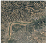
Seasonal rivers and streams are particularly affected by seasonality and partially dry up during the dry season due to insufficient recharge.
Lakes Land 10 01070 i003Permanent freshwater lakes; seasonal/intermittent freshwater lakes (>8 ha *). Could include natural or constructed waterbodies.
Canals Land 10 01070 i004
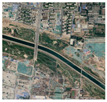
Constructed canals and drainage channels.
Reservoirs Land 10 01070 i005
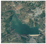
Constructed water storage areas and impoundments (generally > 8 ha *).
Ponds Land 10 01070 i006
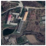
Comparatively small constructed or natural shallow waterbodies (lentic ecosystems) including irrigation ponds, stock ponds, and small water tanks (generally < 8 ha *).
* The 8 ha cut-off between ponds and lakes was consistent with the classification used by the National Wetland Resources Survey.
Table 2. Correlation coefficients (lower half of matrix) and p-values (upper half of matrix) between possible drivers of waterbody change. Bolded correlation coefficients are significant at p ≤ 0.05. Variables include built-up area (BUA), length of water pipeline (LWP), population density (PD), potential evapotranspiration (PET), average monthly precipitation in the 6 months prior to satellite images capture (PRCP6), average monthly precipitation in the 12 months prior to satellite images capture (PRCP12), and annual mean temperature (AMT).
YearBUALWPPDPETPRCP6PRCP12AMT
Year 0.00030.0009<0.00010.01710.73830.46330.0004
BUA0.9694 0.0002<0.00010.0460.89320.33060.0012
LWP0.95380.9738 0.00040.02960.93760.34670.0002
PD0.98620.98380.9656 0.03050.9340.50920.0001
PET0.84350.76310.8030.8007 0.48520.34280.031
PRCP6−0.1560.0631−0.0368−0.0389−0.3193 0.66250.7472
PRCP120.33450.4340.42110.30280.42430.203 0.6363
AMT0.9650.94640.97220.97780.7993−0.15060.2195
Table 3. The overall accuracy and kappa coefficients for the waterbody classification.
YearOverall AccuracyKappa Coefficients
199093%0.91
199592%0.89
200093%0.90
200595%0.93
201087%0.83
201589%0.84
202096%0.94
Table 6. Number of waterbodies in each category that are in the top 100 for each aspect of landscape connectivity (dPCintra, dPCconnector, and dPCflux). The perennial river was excluded to better understand the changes in connectivity of the other waterbody types in Zhengzhou.
dPC IndexWaterbody Type1990199520002005201020152020
dPCintraSeasonal rivers and streams43454239364729
Canals7687121326
Lakes3759121320
Reservoirs46374045402725
Ponds1550000
dPCconnectorSeasonal rivers and streams85827972536535
Canals9132016372957
Lakes0003018
Reservoirs65191050
Ponds0000000
dPCfluxSeasonal rivers and streams66717158516340
Canals11131113271541
Lakes222351115
Reservoirs2114162617114
Ponds0000000
Publisher’s Note: MDPI stays neutral with regard to jurisdictional claims in published maps and institutional affiliations.

