Dependencies between Demographic Urbanization and the Agglomeration Road Traffic Volumes: Evidence from Poland

Abstract

A method is proposed for forecasting traffic intensity at the border of an agglomeration’s core, using demographic data such as amount (number) and structure of population and housing in the surrounding (suburban) area. Relationships between groups of variables are analyzed by calibrating traffic and demographic models for a selected agglomeration in Poland. The choice of Poland is justified by an intensive suburbanization process that took place during the transition from a centrally controlled market to a free market economy after 1989, such research being quite novel and original for this country. Three assumptions concerning this research methodology (concerning how to specify the research area and parameters characterizing traffic and population) were formulated and tested. Models (dependencies) acquired this way were tested in another Polish agglomeration of similar size, yielding similar results. Very high correlations between characteristic groups of variables were indicated. The best correlation occurred between an intensity of cars leaving the center of an agglomeration in the afternoon rush hour (as a traffic group variable), with the total population, the number of economically active people, and the number of dwellings in the surrounding areas (being population group variables). A novel way of specifying the range of the surrounding areas influencing the main city traffic was proposed. The results obtained and the models constructed should be applicable for other agglomerations, since the universality of the observed phenomena and their relationships are expected.

1. Introduction

Groups of communes investigated in this paper as an “agglomeration” will be analyzed as an interacting pair of a core (main city) and its surroundings (villages and cities neighboring the core). The term “suburbanization” is understood, in general, as a development of the surroundings while the core is dwindling or stable.

The diverse processes of suburbanization (social, economic, morphologic, etc.) in the world has been ongoing since the 1960s, and in Central and Eastern Europe they developed with greater intensity after 1989 [1], when this region was freed from the strict zone of control of the Soviet Union and the communist system fell. The choice of Poland is therefore important because of an intensive suburbanization process that took place during the transition from a centrally controlled to a free market economy after 1989. Such studies are unprecedented for Poland, in part because of limited availability of data, which is discussed below. The economic transition caused land use, and specifically land rent, in spatial development and urban planning to become an important factor in these countries [2,3]. The transition also triggered a rise of wealth within the society, an increase in mobility and motorization, and finally a change in social attitudes related to a perception of quality of life as an important criterion for living [4,5,6]. They were the same factors that caused urbanization of the core cities’ surroundings in Western European and North American countries [7,8]. As in these countries, suburbanization primarily took place in the richest centers, which were successfully—in economic terms—undergoing transformation [9].

The issues of suburbanization are a subject of numerous studies, conducted from the position and with the use of social (human geography, sociology, economics), natural (ecology, biogeography), and technical (transport engineering, urban planning) methods. In this paper the main focus is given to spatial (geographical) and transport issues. For this purpose, the most general definition of suburbanization was adopted, defining it as a process in which the population is shifted from the core (central urban) areas to their respective surrounding areas (suburbs), resulting in the formation of an urban sprawl. As a consequence of these migratory movements of households and business entities away from the core, the surrounding urban areas grew [10].

Suburbanization has its specific demographic, morphological, social, economic, and technical dimensions [11]. There is no singular commonly accepted model of suburbanization. In the context of the phenomena discussed in this paper, the phase model [12], in which suburbanization is a next step of a wider, more general process of urbanization, deserves attention. Attempts to model the spatial structure of settlement location in the surroundings are also noteworthy, in which such forms and processes, known as “frog leap,” “concentric,” “ribbon development,” “one-off housing,” etc., are distinguished [13,14]. The surroundings themselves are also not unambiguous, with terms such as “suburban area,” “peri-urban area,” and “rural-urban fringe” being used. The essence of distinguishing these areas is the transient nature of their use and function, associated with a permeation of areas with urban and rural characteristics [15].

The specificity of suburbanization in European countries that before 1989 were in the Soviet Union’s sphere of control, including Poland, is that it generally occurs in a spontaneous, poorly organized, and uncontrolled manner. In this regard, the urban sprawl process (which rarely takes the form of random or accidental distribution of settlements in Western countries) in countries such as Poland [16,17], Romania [18], Bulgaria [19], or the former Yugoslavia [20] has grown to sizes unprecedented in other countries. Analyses of this process are not sufficiently sensitive to the needs of the common good [16], which is caused by an ambiguity of administrative regulations dealing with construction investments, especially in the first period of transformation [21], as well as the strong commercial nature of land use.

On the other hand, with the emergence of so-called delayed urbanization [22], or under-urbanization [23], in the new market conditions, inhabitants moving to agglomerations from rural areas chose suburban locations (in contrast to urban locations) because of lower real estate prices and their reluctance to give up the existing “rural” lifestyle [14]. A process was observed in which land, well connected to public roads and the public transport network, was bought much more slowly than land in areas with inferior transportation. This resulted in a large supply of building plots in the suburban areas [24,25], which, with the deficiency of urbanization control, led to an increased scattering of buildings [26,27]. This process is also noticeable in the suburban areas of smaller cities and towns [28,29], as well as in countries where the suburbanization processes seem to be less advanced, such as Ukraine [30].

The dispersion of the built-up areas into the suburban areas (suburbs) moves inhabitants into areas of poor public transport services [31]. The service is poor (sometimes negligible) because operational costs on an excessively fragmented network of lines and stops are too high to maintain an economically feasible public transport system. [10,32]. This results in an increase (hypertrophy) of individual motorization, which in turn degrades the environment, increases traffic congestion, increases travel time with negative consequences for social and family interactions and for people commuting to work, decreases traffic safety (causes additional road accidents), and has other negative effects. This generates huge external costs, estimated for Poland at tens of billions of euros per year [33], which are becoming an increasingly serious development barrier for public finances [34,35].

Due to such negative effects, the problem of the population growth’s impact on transport needs is the subject of numerous studies, both in countries with a stable population [36,37] as well as in countries with rapid urbanization such as China [38]. Research shows strong links between population growth and mobility, although these links are considered non-linear and complicated [39,40]. A question arises whether such dependencies are universal or country-specific, e.g., only for countries with strongly vibrant and spontaneous urban sprawl processes. In this setting, as mentioned, Poland and other countries of Central and Eastern Europe can be characterized by particularly chaotic suburbanization processes and a strong growth in motorization, without effective local rail transport services for most agglomerations [41].

For these reasons, the need to study the relationship between urbanization processes and the traffic (transport) structure and volume is currently extremely relevant. More or less advanced analyses of traffic modelling, carried out so far in different regions of Central and Eastern Europe [42], are, however, too general, and are missing detailed research. They therefore fail to precisely explain the main reason for the increase in local traffic volumes, and how this not-specified reason influences this increase, especially in chaotically developed surroundings.

Taking into account the aforementioned formulation of the problem, the main goal of this paper is to find a relationship between population growth and traffic volume in the area of residential suburbanization, under conditions of uncontrolled (chaotic, scattered, ineffective) urbanization. The goal is not only cognitive and methodical, but also has practical significance. The latter is connected with a possibility to use the research results in a policy for sustainable development of the surroundings.

An influence of the type of buildings and development on the volume (share) of car traffic during times of commuting (access to the core of the agglomeration) has been studied many times [43,44,45,46,47]. Other factors influencing car use, such as the quality of the public transport system, of the cycling infrastructure, or both [48,49,50,51,52], or of the availability of parking lots for cars [53,54], have also been identified.

A comprehensive analysis and comparison of transport indicators was carried out in [55], showing an attempt to define the most important transport and socio-economic indicators from 151 agglomerations and 51 countries and obtaining correlations between infrastructure availability (including accessibility), socio-economic indicators, and congestion levels. The relationship between the development of transport infrastructure and population growth, spatial expansion, and changes of land use was highlighted in many works [56,57,58]. The close link between transport and urban development was also acknowledged in earlier studies [59,60,61]. An imbalance between travel demand and the supply of a transport infrastructure has been identified as a cause of increased congestion [56].

The development of a road network generally leads to a lower population density in the cores [10,62]. Empirical estimates [63] indicate, moreover, that every expansion of a motorway into a core of an American agglomeration results in an average 18% decrease in the number of inhabitants in the core. An analysis in Wisconsin revealed that the expansion of motorways caused population growth in the surroundings and increased urban sprawl [64]. The expansion of the road network tends to reduce the urban density and efficiency of road-based public transport, creating conditions for growth in car ownership. The consequence of these effects is a further increase in the demand for private car use, often referred to as “induced demand” [65].

An inhabitant’s lifecycle proved to be an important factor in the transport mode choice of travel from the surroundings to the core. Experiences from an earlier place of residence [66,67], as well as changes in life situation [68], such as taking up employment after graduation [69], starting a family, or children becoming independent, influences the commuter’s decisions.

2. Research Methods and Source Data

Studies of traffic dependence on population face a number of obstacles, such as obtaining reliable data, comparing study periods and locations, or selecting appropriate variables (parameters). The basic dilemmas can be listed here: where and when to measure traffic, which groups (categories) of vehicles should be taken into account, how to separate transit traffic data, which area of the surroundings should be taken into account, and how to supplement traffic measurements with other surveys (e.g., questionnaires).

In light of additional obstacles in obtaining a complete set of up-to-date and reliable data, presented further on, we looked for a correspondence of parameters not widely used at present, such as the number of personal vehicles in the three rush hours versus the number of the working-age population or the quantity of houses. Our intention was to propose a very simple (but effective) method based on a modest (but obtainable) set of data. As is shown further on (this is shown by a correlation of results for two agglomerations), this method is authoritative for cities in Poland. It is however expected that this method is applicable in other countries, creating a valuable contribution to the research methodology.

For the purpose of this research, the following assumptions were formulated:

A1—While it is important to initially include in a study all inlets to the core (on the border cordon), some of them may be omitted in the study’s subsequent stages.

A2—For correlation analyses specific traffic characteristics can be selected, such as private vehicle peak period intensity, distinguishing a source–destination relationship.

A3—For correlation analyses, specific population characteristics should be taken into account, with a focus on specific groups in the population and with data on housing, as well as with a specification of the surrounding area.

These assumptions allowed us to propose a very simple but effective method for calculating and forecasting traffic intensity at the border of an agglomeration’s core by using a relatively easy obtainable set of data. The adopted method starts with a delimitation of the surroundings (in other papers also referred to as “source area,” “catchment area,” and “suburban area”) based on commuter traffic and the location of services, acquiring demographic and spatial data for this area, followed by a comparison of changes in the intensity of commuter traffic. Thus, the relationship between the traffic volumes recorded at the border of the agglomeration’s core and the data on the population in the surroundings is analyzed. The exact delimitation of the border between the core and the surroundings depends on the location of the traffic measurement points (inlets).

Traffic volume data is represented by 6 variables (VTi): the total number of vehicles per day (VT1), the number of private vehicles per day (VT2), the number of private vehicles during the morning rush-hour period from 06:00 to 9:00 (VT3), the number of private vehicles during the morning rush-hour period from 6:00 to 9:00 only towards the core (VT4), the number of private vehicles during the evening rush-hour period from 15:00 to 18:00 (VT5), and the number of private vehicles during the evening rush-hour period from 15:00 to 18:00 only from the core (VT6).

The traffic data was acquired from official measurements done for the Comprehensive Traffic Analysis (CTA) in the studied areas [70,71,72]. The CTA included traffic measurements on the circumference of specified areas—for this paper data gathered at the circumference of the core was used. In the CTA the intensity of the incoming and the exiting traffic was measured and investigated, differentiating vehicle types and allocating the measured data to every hour or quarter of an hour. Measurements at all locations were done by analysts standing by a roadside or by video filming during 24 h of one spring workday, assisted by measurements on the following days (including weekend days) at chosen locations. The results were confronted with data from other periods and in rare cases, where the difference between measured and anticipated volumes was too big, repeated in the following days. The date of the measurements was arranged with local road authorities to minimize road work in the week the measurement were taken, ensuring undistorted traffic distribution. CTA measurements from earlier years were done at a greater number of locations, covering practically all paved inlets to the core. Measurements done in later years skipped some locations that were considered to have no visible impact on city traffic—this assumption could be verified by automated measurements installed at certain locations, but also acquired from responsive traffic light controllers, for which traffic measurement is an important element. The data from the CTA was used primarily to create a traffic model, but was ready to be used for other purposes, such as the research presented in this paper.

The demographic data used in this paper came from publicly available statistical studies: the number and structure of the population in the years 2010 and 2018, as well as the number of existing and completed houses within the 2010–2018 period, noted for each commune (with a separation of cities and rural areas in urban–rural communes) and registered by the Central Statistical Office in Poland (www.stat.gov.pl). This data was compiled in the form of 5 variables (VPj): total population (VP1), population aged 5–17 (VP2), working age population (VP3), population of post-working age (VP4), and number of houses (VP5).

The data on the population came from the “population balance,” i.e., the current registration, carried out by the relevant municipal offices. This registration consisted of an administrative statement that a certain person was registered. It should be noted here that in Poland the approval of the data (not only population data) quality, timeliness, and relevance is limited. The data quality of population registration (and thus migration) [73], location of buildings and address points [74], and car registration [75], affects various indicators, especially mobility and motorization. Thus, it was not possible to analyze in detail issues such as the impact of household characteristics, professional status, etc., on traffic.

Unfortunately, in Poland, other potentially useful data including the structure of households in communes and smaller units (e.g., statistical regions), are not available (despite censuses). This, however, cannot reduce the importance of research needed for Poland, being the largest country in Central-Eastern Europe, and therefore providing a sufficient data pool for research on such important issues as the cause-and-effect relationships between transport, mobility, and demographic development. These are the key issues in understanding the mechanisms of urbanization in the countries undergoing transformation. Finding regularities and correlations can make a significant contribution to the theory and methodology of developing complex settlement systems such as urban agglomerations, which are the subject of this paper.

3. Characteristics of the Research Area

For the analyses, Wrocław and Poznań agglomerations were selected. The core cities of these agglomerations seem to be quite representative in terms of the suburbanization process in Poland: They are quite large cities (530,000–640,000 inhabitants), constituting the nucleus (“kernel”) of the so-called polycentric settlement system of Poland [3]. In both centers, the surroundings developed quite intensively but unevenly along their perimeter [9,17]. The demographic and economic growth of the surroundings was caused in part by an inflow of foreign investments, which created jobs [76,77]. In both agglomerations the process of “urban sprawl” [78,79], characteristic for the whole of Poland, is common.

For creation of the model, the Wrocław agglomeration was selected, being conditioned by several factors. Firstly, there are comparable traffic measurements for 2010 and 2018 for this area [70,71]. Secondly, the surroundings of Wrocław are characterized by an extremely large intensity of demographic urbanization processes [17], which are related to, among others, numerous investments creating several thousand jobs [76,80]. Thirdly, the agglomeration is well recognized in terms of traffic conditions, development of transport networks, sustainable development, and the phenomenon of urban sprawl [81,82,83,84]. Wrocław is the fourth largest city in Poland with more than 600,000 inhabitants in the core and with the residents of the surroundings approximately doubling this number (creating the “MAX” area).

The research area initially covered 51 units (communes and towns) around Wrocław (“MAX” area), but stage A of the analysis reduced this number to 24 (including Wrocław). Communes distant from the core were rejected due to the lower intensity of mutual relations expressed by lower dependence values. For further analysis, such reduced catchment areas, called the “Inner Area,” turned out to be significant—this area covered the communes surveyed in the Comprehensive Traffic Analysis (“KBR” area, year 2018), but accompanied two other communes. The towns in seven urban–rural communes that are not separate communes were analyzed both as parts of communes and as independent units. The topography of the “Inner Area” is shown in Figure 1. The following units were considered:

• U0—the core of the agglomeration—Wrocław;
• U1–U21—rural or urban–rural communes surrounding the core (including two communes not covered in the Comprehensive Traffic Analysis (2018): U15—Jordanów Śl. and U17—Sobótka);
• U22 and U23—two urban communes; and
• U24–U30—seven towns that are parts of urban–rural communes.

Basic data for the aforementioned units are given in

Table 1. Basic data on the examined administrative units.

Unit Symbol	Unit Name	Area (sq. km)	Population (Thousands of Inhabitants in 2018)
U0	Wrocław	292.8	630.7
U1	Długołęka	212.8	11.7
U2	Czernica	83.6	24.0
U3	Siechnice (with U24 town)	98.7	3.1
U4	Żórawina	120.3	16.8
U5	Kobierzyce	149.3	3.8
U6	Kąty Wrocławskie (with U26 town)	176.7	9.2
U7	Miękinia	179.5	21.0
U8	Oborniki Śląskie (with U30 town)	154.3	6.0
U9	Wisznia Mała	103.4	15.0
U10	Oleśnica (rural commune)	242.9	16.2
U11	Jelcz Laskowice (with U25 town)	167.6	5.3
U12	Oława (rural commune)	234.7	10.9
U13	Domaniów	94.5	12.7
U14	Borów	98.7	7.0
U15	Jordanów Śląski	56.7	0.0
U16	Strzelin	171.4	9.3
U17	Sobótka (with U27 town)	136.3	22.9
U18	Kostomłoty	145.2	19.1
U19	Środa Śląska (with U28 town)	216.0	8.8
U20	Brzeg Dolny (with U29 town)	94.4	10.3
U21	Trzebnica	200.0	5.7
U22	Oleśnica (urban commune)	21.0	9.4
U23	Oława (urban commune)	27.4	15.1
U24	Siechnice (town)	15.6	37.1
U25	Jelcz-Laskowice (town)	167.6	12.3
U26	Kąty Wrocławskie (town)	8.6	6.3
U27	Sobótka (town)	32.2	10.3
U28	Środa Śląska (town)	14.9	13.0
U29	Brzeg Dolny (town)	17.2	5.1
U30	Oborniki Śląskie (town)	14.5	16.5

Source: own research based on Central Statistical Office in Poland data (Local Data Bank) http://bdl.stat.gov.pl/.

. In Figure 1 black lines mark “limited access roads” (motorways and expressways). Urban communes or towns that are parts of urban–rural communes are distinguished in grey. The Odra River is also marked, because outside Wrocław there are only three bridges on the Odra in the analyzed area, so the river is a barrier to traffic. The boundaries of the communes are shown with black lines.

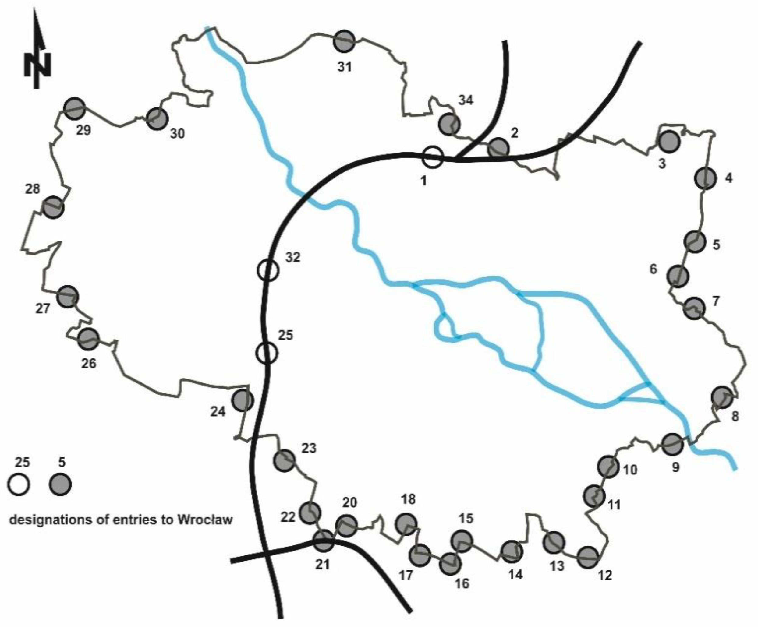
A total of 32 inlets (entries) to the core were identified (Figure 2,

Table 2. Characteristics of inlets to the core (Wrocław) from a survey in the year 2018.

No.	Description of Selected Inlets	ADT [veh./day]	r1 [%]	r2 [%]	r3 [%]
1	Inlet from the motorway	30,900	83	64	22
2		7029	85	77	23
3	State road	14,946	89	52	21
4	State road	35,388	82	56	19
5		15,047	87	60	16
6		8514	89	65	21
7		6856	87	86	31
8	Regional road	21,109	84	56	19
9		3585	90	98	38
10		1753	86	82	29
11	State road	19,868	84	58	16
12		3656	88	91	36
13		3565	84	71	31
14	Regional road	17,630	86	61	17
15		11,972	88	56	18
16		7290	90	75	24
17		8760	90	50	24
18		10,356	88	68	15
20	State road (with access from the motorway south of Wrocław)	62,577	90	49	18
21		16,140	87	49	14
22		3299	86	77	26
23	Regional road (with access from the motorway)	20,318	78	56	20
24		11,636	90	74	18
25	Inlet from the motorway	31,166	84	58	20
26	Regional road (formally)	1952	81	76	21
27		2209	85	80	24
28	State road	17,255	75	54	20
29		2459	81	80	22
30	Regional road (formally)	7844	86	72	20
31	Regional road	12,715	88	72	20
32	Inlet from the motorway	17,262	82	60	21
34		13,376	83	66	17

Source: based on [71].

and

Table 3. Characteristics of inlets from surveys in the year 2010.

No.	Description of Selected Inlets	ADT [veh./day]	r1 [%]	r2 [%]	r3 [%]
2		6492	84	78	25
3		4772	82	75	24
4	State road	36,879	74	58	16
5		10,213	84	57	17
6		4488	88	52	23
7		4524	88	92	38
8	Regional road	17,820	82	64	19
9		424	76	66	22
10		876	72	46	26
11	State road	20,425	81	58	18
12		5472	90	90	33
13		2100	83	64	28
14	Regional road	11,681	83	61	21
16		4852	84	69	22
17		3778	83	45	30
18		5550	90	74	26
20	State road (with access from the motorway south of Wrocław)	65,776	75	50	18
21		21,222	84	52	13
22		768	70	60	20
23	Regional road	13,418	75	68	20
24		7268	88	60	22
26	Regional road (formally)	2508	76	58	26
27		858	84	79	26
28	State road	14,106	74	58	19
29		1628	73	79	27
30	Regional road (formally)	3878	82	71	21
31	Regional road	14,515	85	72	20
34	State road	18,899	74	62	19

Source: based on [71].

). The numbering refers to the one used in the Comprehensive Traffic Analysis [70], hence numbers 19 and 33 are missing. Inlet Nos. 1, 25, and 32 were exits from the AOW (Motorway Bypass of Wrocław). Other inlets were located where roads crossed the core border (or nearby). The classification of these roads (function, agglomeration affiliation, technical class) varied, but they all served agglomeration traffic to a greater or lesser extent. Some of them also served long-distance traffic (“long-distance” meaning the traffic was traveling outside the agglomeration). Table 2 summarizes the basic characteristics of inlets in 2018. Some inlets, on roads of higher categories—national and regional (voivoideship)—for which the share of traffic not related to the core (long distance) was significant, were marked. Some of the regional roads were marked “formally regional road,” because they were formally assigned to be regional, but did not carry supra-local traffic. In addition to the average daily traffic intensity (ADT), the following parameters characterizing the traffic are given:

r1—share (ratio) of private vehicles relative to the total traffic [%];

r2—share (ratio) of the direction to the core relative to both directions in the morning rush-hour period (06:00–09:00) in the private vehicles group [%]; and

r3—traffic share in the morning rush-hour period (06:00–09:00) relative to the daily traffic in the private vehicles group [%].

The current traffic survey (CTA) was made in 2018 for the city (“core”) and for 21 neighboring communities making up the “surroundings.” The surroundings were inhabited by about 364,000 people, including about 336,000 people over six years of age. Data was collected from various sources: surveys taken from households; an online survey; surveys taken from public transport passengers; complementary surveys taken at bus stations, railway stations, shopping centers, municipal entities, universities, and companies; surveys taken from people in public transport vehicles; and car, bike, and pedestrian traffic. A complete description of the survey and access to the database of results are available on the Internet [70], with an English summary. The traffic volume on the core cordon was measured continuously for 24 and 16 h, using conventional measurements and image recording devices (video recorders), allowing the measurements to be archived.

The inlet characteristics for the year 2010 are given in Table 3 in the same way as for the year 2018. The numbering of these inlets was used according to CTA (2018), hence some of them are missing as they did not exist in 2010.

4. Calculations and Analyses

Following an analysis of the traffic surveys [70,71] for all inlets on the border of the core (Wrocław), a preliminary aggregation procedure was done considering the parameters characterizing the traffic described in chapter 2. The results of the aggregation allowed us to identify several groups with characteristic features. It has to be noted that between the years 2010 and 2018 the road network was expanded, significantly increasing capacity and traffic quality of some inlets—changes in traffic distribution caused by this expansion require additional research exceeding this paper’s scope. However, a fourth assumption was made, stating that specific inlets could be aggregated or eliminated to acquire groups “accused” of having specific dependencies from variables describing demographic and spatial characteristics. A total of 12 groups of aggregating inlets were assembled and shown in

Table 4. Groups aggregating traffic parameters for the Wrocław agglomeration.

Group	Aggregated Inlets	Summarized Traffic Intensity (Private Cars Leaving the Core in 3 Afternoon Rush Hours: Thousands of Vehicles) VT6
		Year 2018	Year 2010
T1	All inlets	49,673	30,474
T2	All inlets without 4 with the biggest traffic intensity (1, 4, 20, 25)	31,380	21,833
T3	All inlets without 7 with the biggest traffic intensity (1, 4, 20, 25, 8, 11, 23)	25,964	16,040
T4	“Northwest”, a group of 5 inlets (27, 28, 29, 30, 31)	4644	3830
T5	“Northeast”, a group of 5 inlets (3, 4, 5, 6, 7)	9724	6061
T6	T5 without 1 with the biggest traffic intensity (4)	5904	2923
T7	“East”, a group of 3 inlets (7, 8, 9)	3941	2652
T8	“South”, a group of 10 inlets (11, 12, 13, 14, 15, 16, 17, 18, 20, 21)	18,223	13,456
T9	T8 without 1 with the biggest traffic intensity (20)	11,059	7953
T10	T8 without 2 with the biggest traffic intensity (20, 21)	9112	5820
T11	“Southwest”, a group of 4 inlets (22, 23, 24, 26)	3416	2731
T12	T11 without 1 with the biggest traffic intensity (23)	1950	1237

(T1–T12). For demographic data, 17 groups aggregating administrative units were assembled and shown in

Table 5. Groups aggregating demographic parameters within administrative units.

Set of Units	Aggregated Units	Number of Units	Area (sq. km)	Population (Thousands of Inhabitants in 2018)
P1	U1-U9	9	1278	183.0
P2	KBR area (U1 ÷ U23 without U15 and U17)	21	2992	405.2
P3	MAX area (P2 and additional 27 communes)	50	7037	754.5
P4	U7 + U8	2	334	36.4
P5	U7 + U8 + U19 + U20	4	644	72.3
P6	P5 without U28, U29 and U30	4	598	41.3
P7	U1	1	213	32.2
P8	U1 + U10 + U22	3	588	52.4
P9	P8 without U22	2	345	38.8
P10	U2	1	84	15.6
P11	U2 + U11	2	251	38.9
P12	P11 without U25	2	234	23.1
P13	U3, U4, U5	3	368	53.9
P14	U3, U4, U5, U15, U17	5	561	69.9
P15	P14 without U27	5	546	62.0
P16	U6	1	177	24.6
P17	P16 without U26	1	168	17.7

Source: data based on Central Statistical Office in Poland data (Local Data Bank) http://bdl.stat.gov.pl/.

(P1–P17). Differences between the groups’ content validated assumptions A1–A3 stated in chapter 1 (selection of inlets, traffic parameters, and demographic data).

The results of an analysis of dependencies (here as a simple correspondence between two variables) between changes in traffic and population changes between the years 2018 and 2010, done for pairs of traffic and demographic data groups, are given in

Table 6. Pairs of groups used in the first approach of the analysis.

	P1	P2	P3	P4	P5	P6	P7	P8	P9	P10	P11	P12	P13	P14	P15	P16	P17
T1	X	X	X
T2	X	X	X
T3	X	X	X
T4				X	X	X
T5							X	X	X
T6							X	X	X
T7										X	X	X
T8													X	X	X
T9													X	X	X
T10													X	X	X
T11																X	X
T12																X	X

. For the first approach, 34 pairs were taken for comparison. Values close to 1 represent a high correspondence value between traffic and population changes. Average correspondence values for all pairs showing specified variables are given in

Table 7. Average values of correspondence between VT_i and VP_j in the first approach of the analysis.

	VP1	VP2	VP3	VP4	VP5
VT1	1.208	1.136	1.288	0.959	1.083
VT2	1.268	1.192	1.351	1.007	1.137
VT3	1.213	1.141	1.293	0.962	1.088
VT4	1.204	1.132	1.284	0.956	1.081
VT5	1.294	1.217	1.380	1.027	1.159
VT6	1.277	1.201	1.363	1.014	1.145

.

In the second approach, the analyses excluded groups that had the four inlets with the biggest traffic intensity (1, 4, 20, and 25), reducing the number of group pairs to 17. The results of the second approach are given in

Table 8. Average values of correspondence between VT_i and VP_j in the second approach of the analysis.

	VP1	VP2	VP3	VP4	VP5
VT1	1.149	1.087	1.225	0.902	1.033
VT2	1.199	1.135	1.278	0.941	1.077
VT3	1.178	1.116	1.255	0.923	1.057
VT4	1.155	1.094	1.231	0.905	1.037
VT5	1.205	1.141	1.285	0.944	1.081
VT6	1.184	1.120	1.262	0.927	1.062

, showing that the obtained correspondence values were closer to 1 (the average correspondence value in Table 8 is 1.106, whereas in Table 7 it is 1.169). In the third approach the reduction of the group pairs was continued, eliminating outer administrative units and cities (according to assumption A3). This left only six pairs, but resulted in an even better correspondence value, presented in

Table 9. Average values of correspondence between VT_i and VP_j in the third approach of the analysis.

	VP1	VP2	VP3	VP4	VP5
VT1	1.147	1.083	1.212	0.924	1.030
VT2	1.198	1.131	1.266	0.964	1.075
VT3	1.172	1.108	1.239	0.942	1.052
VT4	1.152	1.088	1.217	0.927	1.034
VT5	1.189	1.125	1.258	0.955	1.067
VT6	1.167	1.103	1.235	0.937	1.047

(the average correspondence value is 1.101). These sets of six pairs of groups were identified as reliable for further analysis and used for correlation investigation in further stages of this work.

The presented analysis confirmed that there existed a dependence between traffic and demographic parameters, proving at this stage assumptions A1–A3. Elimination of specific inlets (with big traffic intensity and large long-distance traffic) and cities (corresponding with Friedman and Gordon’s research showing different travel characteristics between new and traditional neighborhoods [85]), and concentrating on rush hours of traffic limited to private cars, led to more strict correlations between the variable pair groups. The choice of the specific (best) pairs of variables (a pair of traffic and demographic variables) could be done according to a correlation analysis.

5. Correlation Analysis (Pearson’s Coefficient) and a Mathematical Description of Dependence of Traffic Volumes on Population

Considering variables VT_i and VP_i for the chosen six pairs of groups (T2 vs. P1, T4 vs. P4, T5 vs. P8, T7 vs. P12, T9 vs. P15, and T11 vs. P17), Pearson’s correlation coefficients (r_VTVP) were calculated separately for the horizons of years 2010 and 2018. The calculations were done using Equation (1), with k showing the quantity of the correlated data (k = 1…6), and assembled in

Table 10. Pearson’s correlation matrix for the year 2010.

	VP1	VP2	VP3	VP4	VP5
VT1	0.997	0.997	0.998	0.994	0.997
VT2	0.997	0.996	0.997	0.995	0.997
VT3	0.997	0.996	0.997	0.995	0.998
VT4	0.997	0.996	0.997	0.995	0.997
VT5	0.995	0.994	0.995	0.993	0.997
VT6	0.997	0.997	0.997	0.995	0.998

and

Table 11. Pearson’s correlation matrix for the year 2018.

	VP1	VP2	VP3	VP4	VP5
VT1	0.996	0.997	0.996	0.992	0.997
VT2	0.996	0.997	0.996	0.992	0.997
VT3	0.996	0.998	0.996	0.992	0.997
VT4	0.995	0.997	0.995	0.991	0.996
VT5	0.996	0.997	0.996	0.992	0.997
VT6	0.997	0.998	0.997	0.993	0.997

.

$$r_{VTVP}=\frac{{\displaystyle \sum _k}\left(V{T}_k-\overline{VT}\right)\cdot \left(V{P}_k-\overline{VP}\right)}{\sqrt{{\displaystyle \sum _k}{\left(V{T}_k-\overline{VT}\right)}^2}\cdot \sqrt{{\displaystyle \sum _k}{\left(V{P}_k-\overline{VP}\right)}^2}}$$

(1)

For given pairs of variables and for the presented time horizons (years) different correlation coefficient values were obtained. Generally, these values were very large (above 0.99) for all investigated pairs, which proved a very strong dependence between parameters describing suburban population and traffic. The next step was a search for mathematical models describing these dependencies, which should enable, or rather predict, changes in traffic, based on population data or housing developments. As the modeled (dependent variable) parameter, the intensity of private vehicles leaving the core in the afternoon rush-hour period (VT₆) was chosen. Chosen for independent variables were the working-age population (VP₃) and the quantity of houses (VP₅).

For the chosen variable pairs VT₆ with VP₅ and VT₆ with VP₃, and for the two time horizons (the years 2010 and 2018—taken separately and together), linear dependency was identified, in a form shown in Equation (2). Parameters a and b acquired for this equation are presented in

Table 12. Parameters of the investigated model for the Wrocław agglomeration.

Pair of Variables, Year	a	b
VT6, VP5, year 2010	−209	0.465
VT6, VP3, year 2010	−360	0.236
VT6, VP5, year 2018	−233	0.489
VT6, VP3, year 2018	−506	0.296
VT6, VP5, both time horizons taken together	−300	0.483
VT6, VP3, both time horizons taken together	−606	0.273

.

VT_i = a + b ∙ VP_j

(2)

6. Model Verification

The undertaken analyses and their results were verified for another Polish agglomeration, similar to Wrocław. The Poznań agglomeration was chosen, with 530,000 inhabitants living in the core, making the city the fifth largest in Poland, with dynamically developing surroundings. The core is surrounded by a poviat (county; second-level administrative unit) including 17 communes, with a total of 390,000 inhabitants and an expectation for the population to swiftly counterpoise (equalize) the population of the core.

The verification was done for 18 administrative units (the city of Poznań; three other towns—Swarzędz, Luboń, and Puszczykowo; seven urban–rural communes—Buk, Kostrzyn, Kórnik, Mosina, Murowana Goślina, Pobiedziska, and Stęszew; and seven rural communes—Czerwonak, Dopiewo, Kleszczewo, Komorniki, Rokietnica, Suchy Las, and Tarnowo Podgórne) and a road network with inlets into the core shown in Figure 3. The uneven distribution of inlets was caused by local terrain obstacles, such as lakes, the river Warta, big forested areas, and a semicircular railway line around the core—for these reasons inlet 22 was not located on the core’s border. In contrast to Wrocław, all exits from limited access roads were located outside the inlets.

A total of 27 inlets taken for the verification are presented in

Table 13. Characteristics of inlets to the core (Poznań) from the survey in the year 2013.

Inlet No.		Number of Vehicles [veh./h]
		Afternoon Rush-Hour Traffic		VT6 *
		Towards the Core	From the Core
1	State road (with access from the motorway)	1577	2363	6546
2		265	606	1679
3		309	330	914
4		419	539	1493
5	Regional road	601	685	1897
6		305	334	925
7		198	143	396
8		251	871	2413
9	Regional road	818	1202	3330
10		4	53	147
11	Regional road	502	1202	3330
12	State road	1125	2224	6160
13		274	438	1213
14		88	167	463
15		75	133	368
16		66	116	321
17	Regional road (with access from the motorway)	1669	3341	9255
18		188	236	654
19		113	508	1407
20	Regional road (with access from the motorway)	997	1641	4546
21		482	852	2360
22	Regional road (with access from the motorway)	1598	3117	8634
23		377	795	2202
24		152	264	731
25		347	291	806
26		443	602	1668
27	Regional road (with access from the motorway)	754	1574	4360

* Parameter VT₆ (traffic intensity at three rush hours) was evaluated multiplying rush-hour intensity by 2.77 (a value characteristic for the analyzed year and area).

. Data from different time horizons (the years 2006, 2011, 2013, and 2015) provided different sets of parameters, so the year 2013 was chosen because it had the widest data scope [70]. Taken for the investigation was data based on the intensity of private vehicles leaving the core (VT₆) with the working-age population (VP₃) and quantity of houses (VP₅) for Poznań’s surroundings. A selection was made of specified sets of traffic data (

Table 14. Groups aggregating traffic parameters for the Poznań agglomeration in the year 2013.

Group	Aggregated Inlets	Summarized Traffic Intensity (Private Cars Leaving the Core in 3 Afternoon Rush Hours: Thousands of Vehicles) VT6
T1-P	All inlets	68,217
T2-P	All inlets without 5 with the biggest traffic intensity (1, 12, 17, 20, 22)	33,077
T3-P	”North”, a group of 7 inlets (2 ÷ 8)	9717
T4-P	”North-east”—an independent inlet, separated from others by the Warta river and a big forest (9)	3330
T5-P	”East”, a group of 5 inlets (10 ÷ 14)	11,313
T6-P	T5 without 1 with the biggest traffic intensity (12)	5152
T7-P	”West”, a group of 5 inlets (1 + 24 ÷ 27)	14,110
T8-P	T7 without 1 with the biggest traffic intensity (1)	7565

) and population (

Table 15. Groups aggregating demographic parameters (VP₃, VP₅) within administrative units for the Poznań agglomeration in the year 2013.

Set of Units	Aggregated Units	VP3	VP5
P1-P	Agglomeration without the core	227,280	114,642
P2-P	Agglomeration without the core and other towns	146,267	72,526
P3-P	Northern communes of Rokietnica and Suchy Las	20,765	9984
P4-P	Northeastern communes of Czerwonak and Murowana Goślina	29,271	13,325
P5-P	P4–P without the town of Murowana Goślina	22,002	10,087
P6-P	Eastern communes of Swarzędz, Kostrzyn and Pobiedziska	53,843	27,304
P7-P	P6–P without the towns of Swarzędz, Kostrzyn, and Pobiedziska	31,855	16,117
P8-P	Western communes of Tarnowo Podgórne, Dopiewo, and Buk	31,482	15,781
P9-P	P8–P without the town of Buk	27,616	13,819

Source: data based on Central Statistical Office in Poland data (Local Data Bank) http://bdl.stat.gov.pl/.

), in accordance with the method used for Wrocław. Therefore, the specified sets, inlets with the biggest traffic (including long-distance traffic) intensity (”5 max”: 1, 12, 17, 20, and 22), and chosen towns were eliminated.

Using population data for the Poznań agglomeration (from Table 15), the model used (Equation (2)) and parameters identified for the Wrocław agglomeration (Table 12) to calculate hypothetical (model) values of traffic parameters VT₆. These values were then compared with real traffic parameters for the Poznań agglomeration (from Table 14). Data for this comparison and the acquired differences (absolute and in percentage) are given in

Table 16. Differences between modeled and real traffic values for specified pairs of groups. Bold numbers signify three best pairs of groups providing the best results, the best pair being additionally underlined.

Column 1	Column 2	Column 3	Column 4	Column 5	Column 6	Column 7	Column 8	Column 9	Column 10
Pairs of Groups	Real Values			Results from the Model (Equation (2)), Values a and b for Year 2010		Difference Between Values from
						Column 4 and Column 5		Column 4 and Column 6
	VP3	VP5	VT6	VT6 = f(VP3)	VT6 = f(VP5)	Absolute	[%]	Absolute	[%]
P1–P, T1–P	227,280	114,642	68,217	53,278	53,100	−14,939	−21.90	−15,117	−22.16
P2–P, T1–P	146,267	72,526	68,217	34,159	33,516	−34,058	−49.93	−34,701	−50.87
P1–P, T2–P	227,280	114,642	33,077	53,278	53,100	20,202	61.07	20,023	60.54
P2–P, T2–P	146,267	72,526	33,077	34,159	33,516	1082	3.27	439	1.33
P3–P, T3–P	20,765	9984	9717	4541	4434	−5177	−53.27	−5284	−54.37
P4–P, T4–P	29,271	13,325	3330	6548	5987	3218	96.66	2658	79.82
P5–P, T4–P	22,002	10,087	3330	4832	4481	1503	45.14	1152	34.60
P6–P, T5–P	53,843	27,304	11,313	12,347	12,487	1034	9.14	1175	10.38
P7–P, T5–P	31,855	16,117	11,313	7158	7285	−4155	−36.73	−4027	−35.60
P6–P, T6–P	53,843	27,304	5152	12,347	12,487	7195	139.64	7335	142.37
P7–P, T6–P	31,855	16,117	5152	7158	7285	2006	38.93	2133	41.40
P8–P, T7–P	31,482	15,781	14,110	7070	7129	−7041	−49.90	−6981	−49.48
P9–P, T7–P	27,616	13,819	14,110	6157	6217	−7953	−56.36	−7894	−55.94
P8–P, T8–P	31,482	15,781	7565	7070	7129	−495	−6.54	−436	−5.76
P9–P, T8–P	27,616	13,819	7565	6157	6217	−1407	−18.61	−1348	−17.82

. For specified pairs of groups referring to the utilization (or not) of each of the assumptions A1–A3, a correspondence of model and real results were acquired. Such correspondence allowed for a final evaluation of the proposed methodology and model, and to direct further research.

A very high correspondence of the model with the real (measured) values was acquired for the whole catchment area, but excluded towns (P2–P) and selected inlets (T2–P: eliminating five inlets with the biggest traffic intensity). This proved assumptions A1 and A3 (assumption A2 was proved earlier). Unfortunately, for other pairs of groups the correspondence was lower: Only for two other pairs was the difference smaller than 10 percentage points. One of these pairs correlated with a chosen direction (set of communes, including a town) with appropriate inlets (including one with big traffic intensity); the second pair also included a town, but without a big traffic inlet.

Finally, parameters for the model (Equation (2)) were calculated for data from Poznań in the year 2013.

Table 17. Parameters of the investigated model for the Poznań agglomeration.

Pair of Variables, Year	a	b
VT6, VP5, year 2013, 3 best pairs	−352	0.459
VT6, VP3, year 2013, 3 best pairs	−137	0.226
VT6, VP5, year 2013, 8 pairs	−765	0.562
VT6, VP3, year 2013, 8 pairs	−918	0.283

presents the values of the a and b parameters, shown separately for the three best pairs and for the addition of the following five pairs of compared groups of data. The obtained results and their dispersion caused some uncertainty about the usefulness of the model. For the three best pairs, the results from Poznań were similar to the results from Wrocław, whereas the addition of the following pairs provided separate values. Further research is therefore required, extending the methodology, which currently is sufficient only for analyzing a full perimeter of the agglomeration’s core.

7. Discussion

Numerous studies included and investigated dependencies between a built environment and travel (i.e., [86,87,88,89]). Ewing and Cervero [90] found more than 200 such studies. Naess [91] stated that there is a dependence between agglomeration structure and travel behavior in Copenhagen, showing differences between the core and its surroundings, i.e., in population density. As a residential area grows, the distances of travel also grows: A correlation between density and traffic intensity, as shown by the average daily travel factor, was given in [92]. There are selected concrete D-variables (density, diversity, design, destination accessibility, distance to transit) that influence household decisions [93]. A recent study [94] tried to determine which opposing point of view of sprawl and congestion is correct: Their model suggests that an increase in compactness reduces the amount of driving done by inhabitants of such a village, but also concentrates the driving into smaller areas.

Complex models describing the dependency between land use and traffic parameters were developed, as shown above, but all of them need a rich set of concrete and comprehensive data. The major obstacle for such research is to collect sufficient and reliable data sets [86,87,88,89]. A comprehensive analysis requires a selection of the data and a separation of specific groups (variables), e.g., regarding the number of personal vehicles during the rush-hour period (three hours) highlighting their direction (from the core). It is important to include specific inlets (with a recommendation to select and reject phase inlets with maximum traffic at calibration). Collecting population data is a separate problem since statistics are not reliable: A failure to comply with registration obligations (or their absence) results in incorrect population data of a given area—in practice in an underestimation of the number of inhabitants. This problem is especially troublesome in the most residentially attractive agglomerations, in which a strong influx of new residents is observed [25,73] (including Wrocław and Poznań, classified next to Warsaw in the so-called “Big Five” agglomerations of Poland [17,27]). Better results were obtained considering the number of houses, although this may also cause an underestimation (new buildings are often reported to the register after a certain period of delay). In such a situation, the most reliable method is to record houses by field observation [52] and on the basis of unprocessed, “raw,” remote-sensing materials (as the recent research shows, in Poland there is a large share of scattered built-up areas, often single-family houses, and the use of bases such as Corine Land Cover is not appropriate for studying changes in the settlement structure [74]).

Our research shows that the growth of residential and apartment buildings and of the population living in the surroundings allows us to assume a future increase in traffic between the two main agglomeration units: the core and the surroundings. This is especially true for new developments in “virgin” (greenfield) areas. For towns already existing, the construction of new developments is filling existing gaps, therefore in such locations we suggest a cautious application. Focusing on household development, the proposed method is not able to determine other parameters of the forecasted changes in traffic structure, such as, in particular, travel distance, which was quantified in the Copenhagen studies [91]. All the more, it is not possible to predict the structure of this traffic in terms of household decisions [93].

In view of the presented obstacles, our method provides a possibility to use selected and easy-to-collect data to approximate the correspondence between the number of people and the passenger-car traffic volume in the border of an agglomeration’s core. The importance of this relationship and its quantification is one of the main current issues in transport and settlement research [90]. The model proved to be feasible for all roads, but the elimination of higher-class roads (leaving only local roads) improved correlation, showing that transit traffic plays a significant role. It also gave a hint that a class of a road might have an influence on traffic volumes, proving assumption A1. On the other hand, this result showed a potential to use the model to evaluate the agglomeration component of traffic on transit roads.

Initially, all traffic crossing the core’s border was taken into consideration, but at the first stage of the analysis the results showed better correspondence when only private (passenger) cars were used, proving assumption A2. Therefore, the volume of cargo vehicles was not investigated in the main study (analysis) of this article. The best results were obtained for private vehicles traveling at rush hours, becoming a welcome outcome: It was the rush-hour traffic that generated the most problems in agglomerations. The evaluation of traffic outside peak hours was therefore less reliable, but such traffic was also less problematic.

The A3 assumption was also proven by showing that not all demographic data showed an appropriate correspondence. The best results were obtained for the quantity of houses and working-age population. This confirmed the results of these studies, which were based on the influence of the age of the structure as the main predicator of changes in the structure of the movement [90].

Suburbanization in the analyzed agglomeration was not homogeneous. Many communes based their success on inviting new inhabitants into housing developments, but some, such as Kobierzyce near Wrocław [76,80,81] and Tarnowo Podgórne near Poznań [78,79], created strong industrial areas. Such differences did not change the feasibility of the model, resulting in the conclusion that in agglomerations with a strongly dominant core, the location of shopping or industrial centers has a small influence on general traffic distribution. On the other hand, the elimination of existing cities—towns with developed urban forms [85]—in the conducted analysis improved correlation values, showing that such suburban cities should be modeled differently. It was also expected that the size of the agglomeration would play an important role—in medium-size cities, location of a large industrial plant might be significant.

Data for the two investigated agglomerations were taken from different years, with the first traffic measurement carried out when limited access roads bypassing the core were absent (under construction). The opening of these bypasses in Poznań and Wrocław did not change the correlation values significantly, allowing us to eliminate circumferential roads (roads directly connecting the dwellings of the surroundings) from considering their influence on the proposed model’s results.

The methodology was generally successful for the whole catchment area. However, for specified inlets, or groups of inlets, it could not be clearly verified. Such a defect might have been caused by specific details skipped in the analysis, such as the mixing and interweaving of agglomeration traffic, making it difficult to assign inlets or groups of them to certain communes or groups of them. Better results were obtained when inlets with large traffic intensity were excluded, which gives an indication on the need to explore the influence of a roads’ technical parameters: Since better roads outside the core lead to better roads inside the core, drivers might not choose the shortest, but rather the fastest option. Terrain obstacles may also play a role: A forest divides the Suchy Las commune into two disconnected parts (to travel between those parts a driver has to ride through the core, crossing two inlets). These deficiencies within the model show a need for further research, using larger data sets and different time horizons for other agglomerations. Such research would be justified by the frequency of this phenomenon, signaled in other agglomerations, especially those located in the vicinity of large undeveloped areas, e.g., forests [29]. As the review of the studies [90] indicated, the travel variables are generally inflexible in relation to the increase in population and to the area of residential and apartment buildings, which may result from specific land-use characteristics.

Nevertheless, on the basis of the performed research, intriguing relationships between traffic intensity on the perimeter of the core’s border and data on the surrounding population were discovered. These dependencies were similar for two considered agglomerations, despite the obstacles indicated above and different periods of research. High correlations of specific variable pairs were obtained and model parameters were estimated. Preliminarily and indicatively, it can be assumed that the traffic outgoing from the core in the rush-hour period (the number of private vehicles) is about half the number of houses and about a quarter of the working-age population. This allows us to estimate the amount of traffic in relation to current and future parameters of the surrounding environment using simple, linear relationships. Such evaluation possibilities are important, since dynamic growth population in the surroundings of Polish agglomerations is very distinct; for example, some communes near Wrocław increased their population by 42% over 10 years.

In addition to the listed advantages of the proposed method, its limitations should also be indicated. Above all, it was difficult to carry out a more advanced modeling of the impact of factors on traffic intensity resulting from the socio-occupational structure of the population. Such modeling was conducted in Poland on a much larger scale for the estimation of traffic on major roads [95], where it was shown that over longer distances the position of a locality in the settlement system and the directions of migration (i.e., the origin of the population) are important for traffic intensity. It should also be noted that the developed method is poorly suited for the analysis of very small spatial units (e.g., statistical micro-areas), and the scale of a district or commune (a few dozen or so sq. km) seems optimal. The results of analyses on the basis of the presented method are also sensitive to a large portion of transit traffic, which has repeatedly been a methodological and interpretative problem (so-called travel flexibility) in many other studies [90].

The development of the proposed method is closely related to the initial assumptions. In future, it is worth examining in more detail which entrances to the city (characteristics resulting from, for example, geographical location) influence the higher or lower correlation score (assumption A1). It would also be worthwhile to examine the effect the choice of time intervals has on the accuracy of the results (assumption A2). It would be interesting to have an accurate variate of the biological structure of the population (assumption A3), especially in the situation described at the beginning of the study where there was no detailed data on the structure of households or the work of residents. It also seems that further development of the methodology in relation not only to the number and structure of the population in a given area (commune), but also to the characteristics of its spatial distribution, i.e., patterns of concentration and dispersion of housing development, has a particularly high research potential. This should be important for the study of agglomerations in post-communist countries [2,6,9,19], where the dispersion of built-up areas is larger [4,15] than in Western European and generally in highly developed countries [7,8]. The conducted research also brings important conclusions of the application of nature, related to local development policy. Very similar correlations found between population growth and traffic volume in two large agglomerations in Poland may be helpful for other centers where there are no traffic measurements (especially on cordons). Knowing these correlations and regularities may allow for better planning of transport policy in relation to recorded population changes. Demographic forecasts are of particular importance here: The results of the studies also provide arguments for limiting the pace of development in areas where transport systems are not yet sufficiently developed.

8. Conclusions

Because obtaining reliable data in Poland might be a problem, including data on where people live or to which commune cars should be registered, crippling the quality of motorization factors, it became necessary to develop a method that would eliminate these difficulties. Therefore, an attempt was made to propose a simple but effective method using a modest but adequate and easily available set of data. The correlation analysis for two agglomerations shows that this method is reliable, at least for agglomerations in Poland. It improves research and modeling methodology, but should be verified in other countries.

It is also important to indicate the legitimacy of integrating the analyzed inlets to the core. This is a clear contribution to the agglomeration travel modeling and deserves presentation and verification by other researchers at other centers. The use of a more complex statistical apparatus is not necessary in this case.

An analysis of the increase in the number of houses and residents allows forecasting changes in traffic volumes at the perimeter of the core’s border and in its interior. If an average occupancy of a private vehicle is known, the model makes calculations of the number of people traveling by car through the perimeter of the core’s border possible. The above parameters are crucial in the planning of urban mobility, determining investment tasks, and striving to balance transport in agglomerations.

The proposed method was tested for parameters giving the best correlation results. Other parameter sets also provided good (although not as high) correspondence. The method should therefore make it feasible to also evaluate other parameters, such as morning or daily (not only rush-hour) agglomeration traffic.

The model was created and tested at two agglomerations of approximately 1 million inhabitants each, with their cores dominating over surrounding communes. This domination neglects the influence of economic differences between these communes on the traffic model. Such differences might be significant if the core’s influence is comparable to the influence of some surrounding communes.