Quantifying the Land Use and Land Cover Changes in the Yellow River Basin while Accounting for Data Errors Based on GlobeLand30 Maps

Abstract

Land use and land cover (LULC) change influences many issues such as the climate, ecological environment, and economy. In this study, the LULC transitions in the Yellow River Basin (YRB) were analyzed based on the GlobeLand30 land use data in 2000, 2010, and 2020. The intensity analysis method with hypothetical errors calculation was used, which could explain the deviations from uniform land changes. The strength of the evidence for the deviation was revealed even though the confusion matrixes of the LULC data at each time point for the YRB were unavailable. The results showed that at the interval scale, the land transition rate increased from the first to the second period for all of the upper, middle, and lower reaches. The exchange component was larger than the quantity and shift component, and the gross change was 4.1 times larger than the net change. The size of cultivated land decreased during both intervals. The artificial surfaces gains were active for all three reaches and had strong evidence. A hypothetical error in 93% of the 2000 data and 58% of the 2010 data can explain deviations from uniform transition given woodland gain during 2000–2010 and 2010–2020. Ecological restoration projects such as Grain for Green implemented in 2000 in the upper reaches resulted in the woodland increase.

1. Introduction

Insight into land use and land cover (LULC) change at a watershed scale is meaningful because of the multi-functions provided by the land. This computation is particularly important due to the influence of human activities on the watershed. Changes to watershed land use by urbanization, ecological restoration projects, and agriculture are increasingly of concern [1]. These developments lead to LULC changes that affect the ecological environment, crop yield, and water resources [2]. Therefore, there is a need to quantify the land use processes because of increased human activities in the watershed of developing countries. Assessing data errors could complement systematic analysis of LULC change [3].

The assessment of the LULC change characteristics relies on the methods applied and the data used. Some studies compared LULC data at two time points by producing a transition matrix, which is the basis for calculating metrics that are used to analyze temporal changes of each LULC type. The rows of the transition matrix show the categories at the start of the year, whereas the columns show the categories at the end of the year. Comparison of the elements in the transition matrix can summarize the net quantity changes in each time interval. However, it is unable to perform a systematic analysis of land change processes, such as identifying the processes that are more intensive than random and uniform processes. The intensity analysis approach was developed based on the transition matrix method, which investigates land use change on interval, category, and transition levels [4,5]. Several studies across Asia, Europe, America, and Africa have used the framework of intensity analysis to investigate the process of land use change [6,7,8,9,10,11,12]. Niya et al. [13] investigated LULC dynamics systematically on Qeshm Island using remote sensing, GIS, and intensity analysis. The results showed that intensity analysis could offer informative knowledge on the biggest island in the Persian Gulf. Ekumah et al. [14] examined the LULC transition from 1985 to 2017 in three coastal urban wetlands in Ghana based on the intensity analysis approach. Mwangi et al. [15] analyzed the patterns and processes of LULC changes in the transboundary Mara River Basin in East Africa using intensity analysis, and the findings were useful for developing effective land use strategies.

Many existing studies assumed that the LULC data they used were accurate. Therefore, LULC change detection approaches were applied to examine the processes of LULC change without taking data errors into consideration. However, many counter intuitive temporal land transitions are due to the fact of data errors instead of actually being changes. For example, Quan et al. [16] doubted that some conversions from built-up land to cultivated land might be caused by data errors. Furthermore, the quantity difference indicates the amounts of the categories but ignores the spatial allocation changes of categories. Therefore, the quantity change may be small even when the gross changes are large. That is to say, there is no quantity temporal change when the amount of gain of a category in some place is equal to the amount of loss of the same category in another place [17]. The quantity, exchange, and shift components could be used to complement the intensity analysis method [18]. Limited studies examined how multiple levels of errors in the LULC data could affect the analysis results. For example, Zhang et al. [19] analyzed the land change processes of Yellow River Basin (YRB) using the trajectory method, and did not take data error into consideration. Complementarily, this study quantified the LULC change in the YRB by using the intensity analysis that can account for data error [20]. The confusion matrix is unavailable for GlobeLand30 data from 2000 and 2020 at present, and it is only available at a global extent for data in 2010 [21]. Since the global scale confusion matrix cannot reflect errors in the YRB, thus, in this study, the confusion matrix was unavailable for all of the three time points.

Some previous studies have investigated the processes of LULC change in part or for the whole of the YRB. For example, Xiao et al. [22] analyzed the spatiotemporal land use change in the YRB within Henan Province from 1990 to 2018. The gravity center transfer model and a cross-tabulation matrix were used to investigate the direction and flow of land use changes in their study. Zhang et al. [19] analyzed the spatial patterns of land use transition in the upper, middle, lower reaches of the YRB, respectively, using the traditional trajectory method. Zhang et al. [23] analyzed the speed and degree of land use change during 1980–2015 in eight sub-regions of the YRB. Most of these studies used the same land use data set, which was produced by the Chinese Academy of Sciences based on remote sensing data such as Landsat and GF-2 [24,25]. Therefore, the assessment of LULC change using different data sources is meaningful to make a supplement. The GlobeLand30 land cover data with 30 m spatial resolution provide an alternative for such an assessment [26]. The GlobeLand30 is a project implemented by the National Geomatics Center of China [27]. It aims at generating global land cover data for finer resolution data analysis. Until recently, the open-access GlobalLand30 land cover data sets at three timestamps of 2000, 2010, and 2020 for the global scale were available. There are 853 raster data tiles that cover the world in total, and the non-destructive GeoTIFF compression format was adopted. The uncertainties and limitations of 41 regional and 23 global land use data sets were compared, and the results showed that GlobeLand30 and FROM-GLC [28] have the finest spatial resolution at the global extent [29]. Several previous studies on the quality of GlobeLand30 have shown a high accuracy [30,31,32,33,34,35].

In recent years, the YRB has been exposed to intensive human activities and extreme climate events that have led to drastic LULC changes. Several ecological restoration programs have been carried out since 2000. The government of China set ecological protection and high-quality development in the YRB as one of the national strategies in 2019 [36]. Systematic insight into LULC change process is important to supply scientific information for sustainable management of land. However, studies measuring land change are still lacking. This study was designed to address the following questions: (1) What are the size, intensity, and the change components of the LULC transitions for the upper, middle, and lower reaches of the YRB? (2) How could errors in the data affect the LULC change intensities of the YRB from 2000 to 2020? The assessment of LULC change in the YRB would be helpful in optimizing the ecological management strategies in the future.

2. Materials and Methods

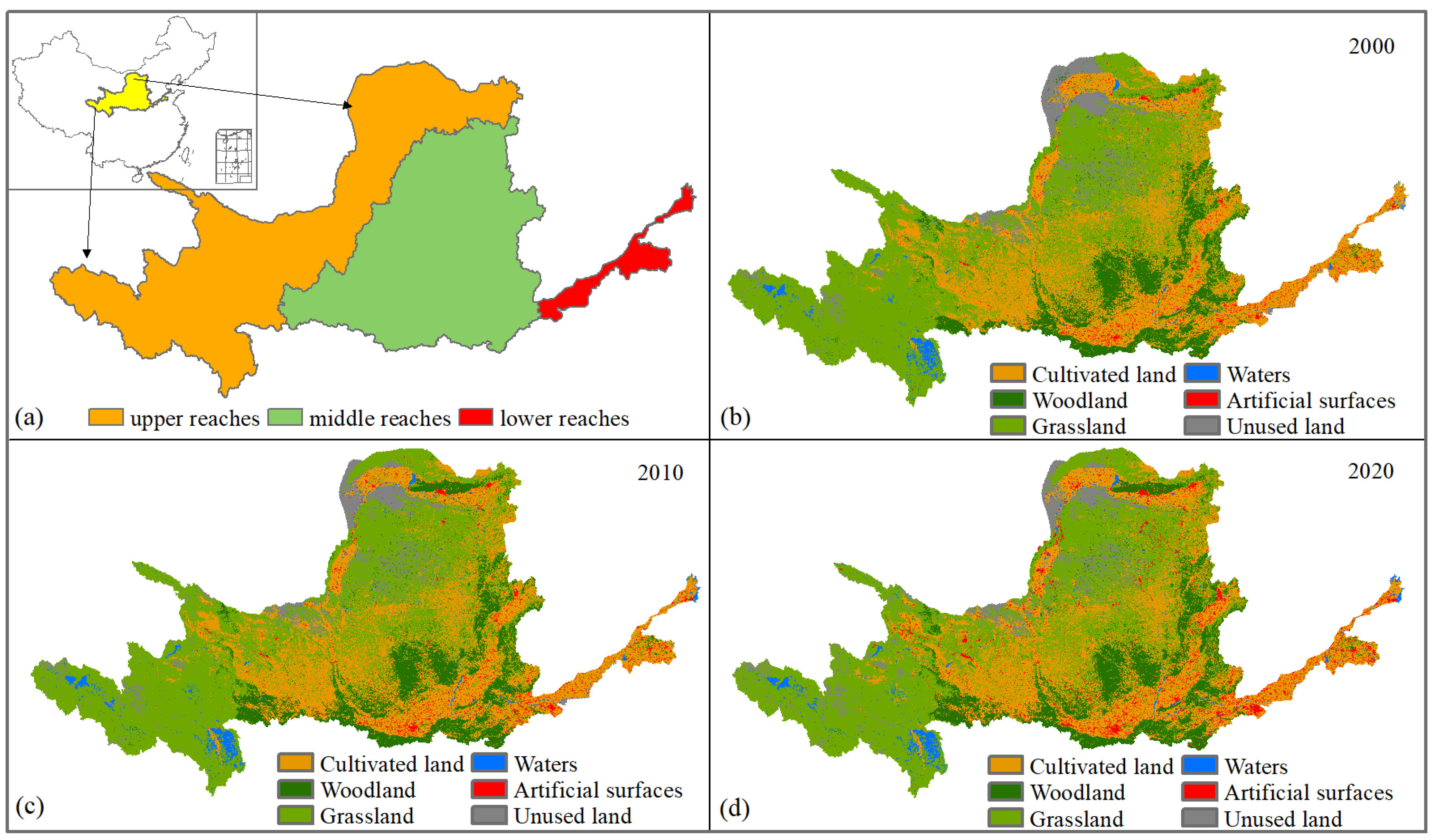
2.1. Study Area

The Yellow River is the fifth largest river worldwide [37]. The Yellow River Basin is the second largest basin in China, supporting 107 million people directly [38]. The YRB is located in northern China (95°53′–119°5′ E, 32°10′–41°50′ N) (Figure 1a), which is also an important ecological barrier in China [39]. It spans nine provinces, and traverses the Tibetan Plateau, the Loess Plateau, Inner Mongolia Plateau, and the North China Plain [40]. The annual mean precipitation ranges from 140 mm in the north to 1100 mm in the east. The annual mean temperature varies from 1 °C in the west to 16 °C in the east [41]. The YRB is located in the typical East Asian monsoon climate zone, and the climate changes from arid and semiarid in the northwest to sub-humid and humid in the southeast. The GDP of the YRB was 23.9 trillion yuan in 2018, which was approximately 26% of the national GDP. The population urbanization rate changed from 38% in 2006 to 54% in 2018 [42]. Over the past several decades, the YRB has experienced the influence of intensive human activities and climate changes that have resulted in serious ecological and environmental issues.

2.2. Land Use and Land Cover Data

The LULC data sets for 2000, 2010, and 2020 at a 30 m resolution from GlobeLand30 were used in this study. The spatial resolution was relatively high for such a large scale. The GlobeLand30 data sets were extracted by the hybrid-pixel and object-based method based on Landsat and HJ-1 satellite imageries [17,43]. In this study, each time point was composed of 11 tiles that were downloaded from the website http://www.globallandcover.com/. The tiles were mosaicked to cover the whole study area for each time point. The GlobeLand30 comprises 10 land cover types: cultivated land, forest, grassland, shrub land, wetland, water bodies, tundra, artificial surfaces, bare land, and permanent snow and ice [44]. In this study, these 10 land cover types were reclassified into six aggregate types, including cultivated land, grassland, woodland, waters, artificial surfaces, and unused land (Figure 1). The reclassification scheme meant that the forest and shrub land were aggregated into woodland, the water bodies and wetlands were aggregated into waters, and the bare land and permanent snow and ice were aggregated into unused land.

2.3. Intensity Analysis

The intensity analysis framework was used in this study. The language R was applied to calculate and plot the data. Detailed information can be found in studies by Aldwaik and Pontius [4,20], Pontius and Santacruz [18], and Pontius [45]. The flow chart (Figure 2) and the main equations are presented as follows.

At the time interval scale, the observed change intensity during year t to year t + 1 was calculated by Equation (1). The uniform change intensity during all time intervals was calculated by Equation (2).

$$S_t=\frac{\mathrm{change}\mathrm{during}[Y_t,Y_{t+1}]/\mathrm{area}\mathrm{of}\mathrm{study}\mathrm{region}}{\mathrm{duration}\mathrm{of}[Y_t,Y_{t+1}]}$$

(1)

$$U=\frac{\mathrm{sum}\mathrm{of}\mathrm{changes}\mathrm{during}\mathrm{intervals}/\mathrm{area}\mathrm{of}\mathrm{study}\mathrm{region}}{\mathrm{duration}\mathrm{of}[Y_t,Y_{t+1}]}$$

(2)

where Y_t and Y_t+1 are years at time point t and t + 1. S_t is the observed change, and U is the uniform change. If S_t was greater than U, then the commission error was computed by Equation (3). If S_t was lower than U, then the omission error was computed by Equation (4).

$$E_t^S=(S_t-U)(Y_{t+1}-Y_t)$$

(3)

$$O_t^S=(U-S_t)(Y_{t+1}-Y_t)$$

(4)

where $E_t^S$ is the commission error, and $O_t^S$ is the omission error. At the categorical level, the annual gain and loss intensity of the categories were computed by Equations (5) and (6), respectively:

$$G_{tj}=\frac{\mathrm{area}\mathrm{of}\mathrm{gross}\mathrm{gain}\mathrm{of}\mathrm{category}j\mathrm{during}[Y_t,Y_{t+1}]/\mathrm{duration}\mathrm{of}[Y_t,Y_{t+1}]}{\mathrm{area}\mathrm{of}\mathrm{category}j\mathrm{at}\mathrm{time}{Y}_{t+1}}$$

(5)

$$L_{ti}=\frac{\mathrm{area}\mathrm{of}\mathrm{gross}\mathrm{loss}\mathrm{of}\mathrm{category}i\mathrm{during}[Y_t,Y_{t+1}]/\mathrm{duration}\mathrm{of}[Y_t,Y_{t+1}]}{\mathrm{area}\mathrm{of}\mathrm{category}i\mathrm{at}\mathrm{time}{Y}_t}$$

(6)

where $G_{tj}$ and $L_{ti}$ are the annual gain intensity of category j and the annual loss intensity of category i, respectively. If the observed gain of j was larger than the uniform change during [Y_t, Y_t+1], then the hypothetical commission of j error at t + 1 (denoted as $E_{tj}^G$) was computed using Equation (7). On the contrary, if the observed gain of j was less than the uniform change during [Y_t, Y_t+1], then the hypothetical omission of j error at t + 1 (denoted as $O_{tj}^G$) was computed by Equation (8).

$$E_{tj}^G=\frac{({\displaystyle {\sum }_{i=1}^J{C}_{tij}})(Y_{t+1}-Y_t)(G_{tj}-S_t)}{100\%-(Y_{t+1}-Y_t)S_t}$$

(7)

$$O_{tj}^G=\frac{({\displaystyle {\sum }_{i=1}^J{C}_{tij}})(Y_{t+1}-Y_t)(S_t-G_{tj})}{100\%-(Y_{t+1}-Y_t)S_t}$$

(8)

$C_{tij}$ is the area that transfers from class i to class j during [Y_t, Y_t+1]. If the observed loss of i was larger than the uniform change during [Y_t, Y_t+1], then the hypothetical commission of i error at t (denoted as $E_{ti}^L$) was computed by Equation (9). On the contrary, if the observed loss of i was less than the uniform change during [Y_t, Y_t+1], then the hypothetical omission of i error at t (denoted as $O_{ti}^L$) was computed by Equation (10).

$$E_{ti}^L=\frac{({\displaystyle {\sum }_{j=1}^J{C}_{tij}})(Y_{t+1}-Y_t)(L_{ti}-S_t)}{100\%-(Y_{t+1}-Y_t)S_t}$$

(9)

$$O_{ti}^L=\frac{({\displaystyle {\sum }_{i=1}^J{C}_{tij}})(Y_{t+1}-Y_t)(S_t-L_{ti})}{100\%-(Y_{t+1}-Y_t)S_t}$$

(10)

At the transition level, when the transitions to category n are examined, Equation (11) gives the observed transition intensity from category j to n (denoted as R_tin). Whereas Equation (12) gives the uniform intensity for class n if n gains uniformly across the study area (denoted as W_tn).

$$R_{tin}=\frac{\mathrm{area}\mathrm{of}\mathrm{transition}\mathrm{from}i\mathrm{to}\mathrm{n}\mathrm{during}[Y_t,Y_{t+1}]/\mathrm{duration}\mathrm{of}[Y_t,Y_{t+1}]}{\mathrm{area}\mathrm{of}\mathrm{category}i\mathrm{at}\mathrm{time}{Y}_t}\times 100\%$$

(11)

$$W_{tn}=\frac{\mathrm{area}\mathrm{of}\mathrm{gross}\mathrm{gain}\mathrm{of}\mathrm{category}n\mathrm{during}[Y_t,Y_{t+1}]/\mathrm{duration}\mathrm{of}[Y_t,Y_{t+1}]}{\mathrm{area}\mathrm{that}\mathrm{is}\mathrm{not}\mathrm{category}n\mathrm{at}\mathrm{time}{Y}_t}\times 100\%$$

(12)

When the transitions from category m are examined, Equation (13) gives the observed transition intensity from category m to j (denoted as Q_tmj). Whereas Equation (14) gives the uniform intensity for class m if m gains uniformly across the study area (denoted as V_tm).

$$Q_{tmj}=\frac{\mathrm{area}\mathrm{of}\mathrm{transition}\mathrm{from}m\mathrm{to}j\mathrm{during}[Y_t,Y_{t+1}]/\mathrm{duration}\mathrm{of}[Y_t,Y_{t+1}]}{\mathrm{area}\mathrm{of}\mathrm{category}j\mathrm{at}\mathrm{time}{Y}_{t+1}}\times 100\%$$

(13)

$$V_{tm}=\frac{\mathrm{area}\mathrm{of}\mathrm{gross}\mathrm{loss}\mathrm{of}\mathrm{category}m\mathrm{during}[Y_t,Y_{t+1}]/\mathrm{duration}\mathrm{of}[Y_t,Y_{t+1}]}{\mathrm{area}\mathrm{that}\mathrm{is}\mathrm{not}\mathrm{category}m\mathrm{at}\mathrm{time}{Y}_{t+1}}\times 100\%$$

(14)

If the transition from i was larger than the uniform gain of n, then the commission of category i error at t (denoted as $E_{tin}^R$) was calculated by Equation (15). On the contrary, if the transition from i was less than the uniform gain of n, then the omission of category i error at t (denoted as $Q_{tin}^R$) was calculated by Equation (16).

$$E_{tin}^R=\frac{({\displaystyle {\sum }_{j=1}^J{C}_{tij}})(Y_{t+1}-Y_t)(R_{tin}-W_{tn})}{100\%-(Y_{t+1}-Y_t)W_{tn}}$$

(15)

$$O_{tin}^R=\frac{({\displaystyle {\sum }_{j=1}^J{C}_{tij}})(Y_{t+1}-Y_t)(W_{tn}-R_{tin})}{100\%-(Y_{t+1}-Y_t)W_{tn}}$$

(16)

Similarly, if the transition to j was larger than the uniform loss of n, then the commission error at t + 1 (denoted as $E_{tmj}^Q$) was calculated by Equation (17). On the contrary, if the transition to j was less than the uniform loss of n, then the omission error at t + 1 (denoted as $O_{tmj}^Q$) was calculated by Equation (18).

$$E_{tmj}^Q=\frac{({\displaystyle {\sum }_{i=1}^J{C}_{tij}})(Y_{t+1}-Y_t)(Q_{tmj}-V_{tm})}{100\%-(Y_{t+1}-Y_t)W_{tm}}$$

(17)

$$O_{tmj}^Q=\frac{({\displaystyle {\sum }_{i=1}^J{C}_{tij}})(Y_{t+1}-Y_t)(V_{tm}-Q_{tmj})}{100\%-(Y_{t+1}-Y_t)V_{tm}}$$

(18)

In addition, the overall difference between land use data at two time points comprises three components: quantity, shift, and exchange. The exchange and shift components are allocation differences. Exchange difference is caused by pairwise confusion, whereas shift component is caused by non-pairwise confusion. A clear description on the calculation processes is illustrated in previous studies [18,45].

3. Results

3.1. Interval Level

In this study, we examined the LULC change in the upper, middle, and lower reaches of the YRB during two time intervals. Each interval had the same time duration (2000–2010, and 2010–2020). The change rate was faster from 2010 to 2020 than from 2000 to 2010 for all of the three reaches (Figure 3a). The change rate was fastest in the lower reaches during 2010 to 2020 with a change percentage of 14.58% of the lower reaches. The LULC change in the upper reaches was the smallest among the three reaches. The commission of change errors were 1.42%, 4.57%, and 1.94% for the domain for the upper, middle, and lower reaches, which can explain the change rate from 2010 to 2020 being larger than the uniform change rate. Instead, the omission of change errors were 1.19%, 2.49%, and 1.44% of the domain for the upper, middle, and lower reaches, which could explain the change during 2000–2010 going slower than the uniform change rate. Figure 3b shows the gross changes during each interval for the three reaches, including the three components: quantity, exchange, and shift. Nearly fifteen percent of the middle and lower reaches showed an overall difference during the second period, and the temporal changes of the upper reaches were relatively less. The exchange was the largest component during both intervals for all reaches except the lower reaches during the second interval. The shift was the smallest component during the two intervals for all three reaches. The quantity components for the upper reaches were much larger than the other two reaches during both intervals.

3.2. Category Level

Figure 4 shows the change intensity of the gains and losses of each category for the upper reaches of the YRB. If a category’s bar ends before the uniform intensity line, then the loss or gain intensity of this category was dormant. On the contrary, if a category’s intensity is larger than the uniform intensity line, then the change intensity of this category was active. Figure 5 shows the size of the gains and losses of all LULC types along with commission or omission errors at the category level for the upper reaches. The observed change for each active category’s gains and losses was the union of the commission error and uniform change. Meanwhile, the union of observed annual gain size and hypothesized omission error size was uniform change size. The grassland experienced larger gain and loss than other categories in terms of size. However, the gain and loss intensities of grassland during both intervals were dormant. The reason was due to the large area of grassland, which accounts for 66.0%, 64.9%, and 62.2% of the total area of the upper reaches in 2000, 2010, and 2020, respectively. The large size of grassland in the denominator produced the small intensity. The gain of artificial surfaces was the most intensively active category during 2010–2020, while the gain of woodland was the most intensively active category during 2000–2010. Furthermore, the error analysis showed that artificial commission error during 2010–2020 was the largest (Figure 5b). That is to say, the evidence for the conclusion of active gain of artificial surfaces was strong. For the upper reaches of the YRB, the change in intensity of woodland was larger than cultivated land during both intervals (Figure 4 and Figure 5).

The categorical level change intensities and sizes for the middle reaches of the YRB are shown in Figure 6 and Figure 7, respectively. The uniform change intensity was 1.46 during 2010–2020, which was 2.65 times higher than for the period 2000–2010 (0.55). During 2000–2010, the intensities of waters’ losses and gains were larger than other changes, but the change in the sizes of waters was small. The reason was that the proportion of waters in the total area of middle reaches was small (0.53%, 0.51%, and 0.59% for 2000, 2010, and 2020, respectively). It was the same as the upper reaches, where the artificial surfaces were also the most intensively active category during 2010–2020 for the middle reaches. The left side of Figure 7 demonstrates where a class error of 50.4% in the 2010 data can explain the differences between the observed gain intensities and the uniform intensity for the time interval 2000–2010. Meanwhile, the class error of 50.1% in the 2000 data can explain the divergences between the observed loss intensities and uniform intensity for the time interval of 2000–2010. The right side of Figure 7 demonstrates where a class error of 45.4% in the 2020 data can explain the differences between the observed gain intensities and the uniform intensity for the time interval 2010–2020. Meanwhile, the class error of 28.2% in the 2010 data can account for the deviation of the observed loss intensities from uniform intensity for the time interval of 2010–2020. Specifically, if the actual commission error intensity for woodland in 2010 was lower than 6.9%, then it could be inferred that woodland was actively gaining. Likewise, if the real omission error intensity for woodland in 2000 was lower than 57.5%, then it could be inferred that woodland was dormant in loss during 2000–2010. The logic is the same for all land use types.

The categorical level change intensity and change area on gains and losses are presented in Figure 8 and Figure 9, respectively, for the lower reach of YRB. Four dormant categorical changes during 2000–2010: cultivated land gain, unused land loss, cultivated land loss, and unused land loss are shown in Figure 8a. All other categorical changes were active. During 2010–2020, three dormant categorical changes were indicated: cultivated land gain, cultivated land loss, and artificial surface loss. All other changes were shown to be active. Therefore, cultivated land was the only category which had a gain and loss that were dormant during both time intervals in the lower reaches. During 2010–2020, the intensity of artificial surfaces gain was larger than the gains of other categories. The cultivated land loss was the largest in terms of area size. However, the intensity of cultivated land loss was less than the other four categories. The reason was due to the large area of cultivated land, which accounted for 80.6%, 76.8%, and 71.0% of the total area of the lower reaches in 2000, 2010, and 2020, respectively.

Figure 10 shows the difference sizes for each LULC type along with the sizes and intensities of difference components for the upper reaches. The red dashed vertical line is the quantity overall line, which indicates the mean value of the quantity proportion in the difference overall for each category. For the time interval of 2000–2010, the grassland accounted for the largest difference, and the exchange component was largest among the three components. In addition, for cultivated land loss, waters gain, artificial gain, and unused loss, the exchange component was also the largest. For the time interval of 2010–2020, the grassland and cultivated land accounted for the largest differences.

For the middle reaches, artificial surfaces change during 2010–2020 was the only category that had a quantity component that was larger than the exchange component. For other LULC types, exchange components were larger than the quantity and shift components during both time intervals (Figure 11). During 2000–2010, cultivated land experienced the largest change due to the large cultivated land gain and even larger cultivated land loss. Whereas during 2010–2020, the change size of grassland was the largest due to the fact of its large gain and even larger loss. For the time interval 2010–2020, the quantity overall line showed that the quantity overall was 11.2% of difference overall, and the quantity + exchange overall was 95.3% of difference overall. Therefore, the exchange component and shift accounted for 84.1% and 4.7% of the difference overall.

For the lower reaches of the YRB, the cultivated land change was largest in terms of size during the two periods, followed by artificial surfaces. The quantity component of cultivated land was more intensive than the quantity overall during the first time interval but became less intensive than the quantity overall during the second time interval (Figure 12). The net changes of all LULC types were stationary through time except grassland and unused land. The quantity changes of grassland and unused land were gains during the first time interval and turned to loss during the latter time interval.

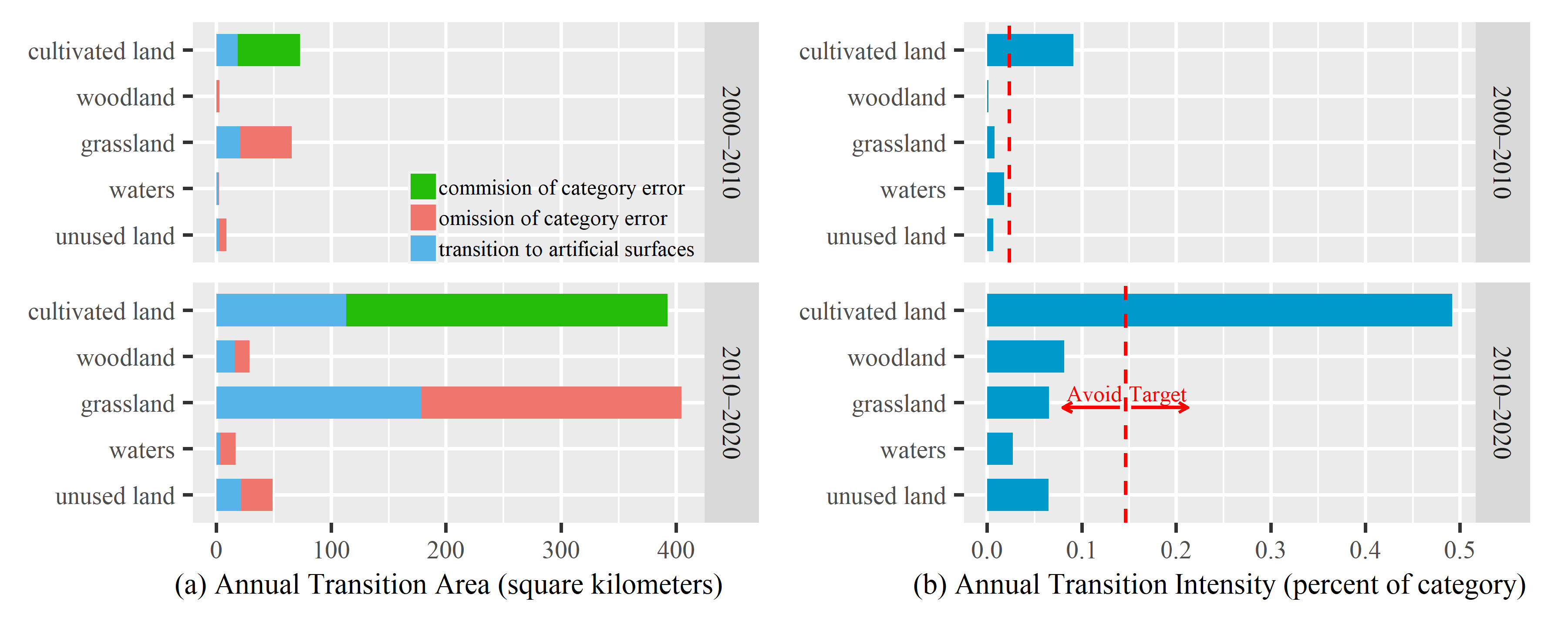
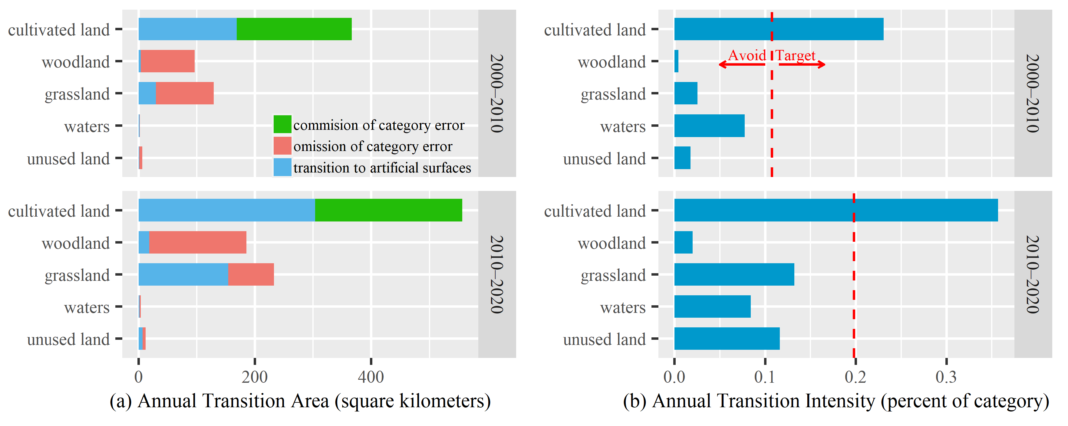
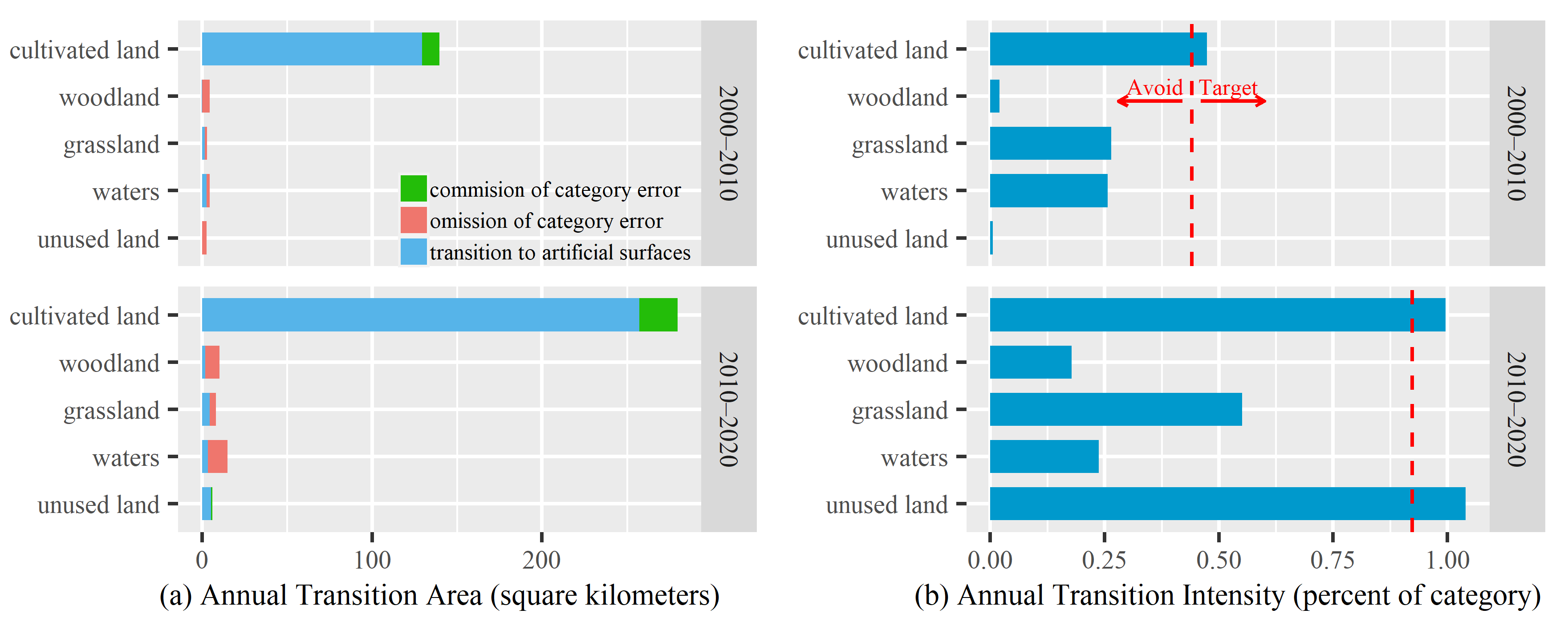
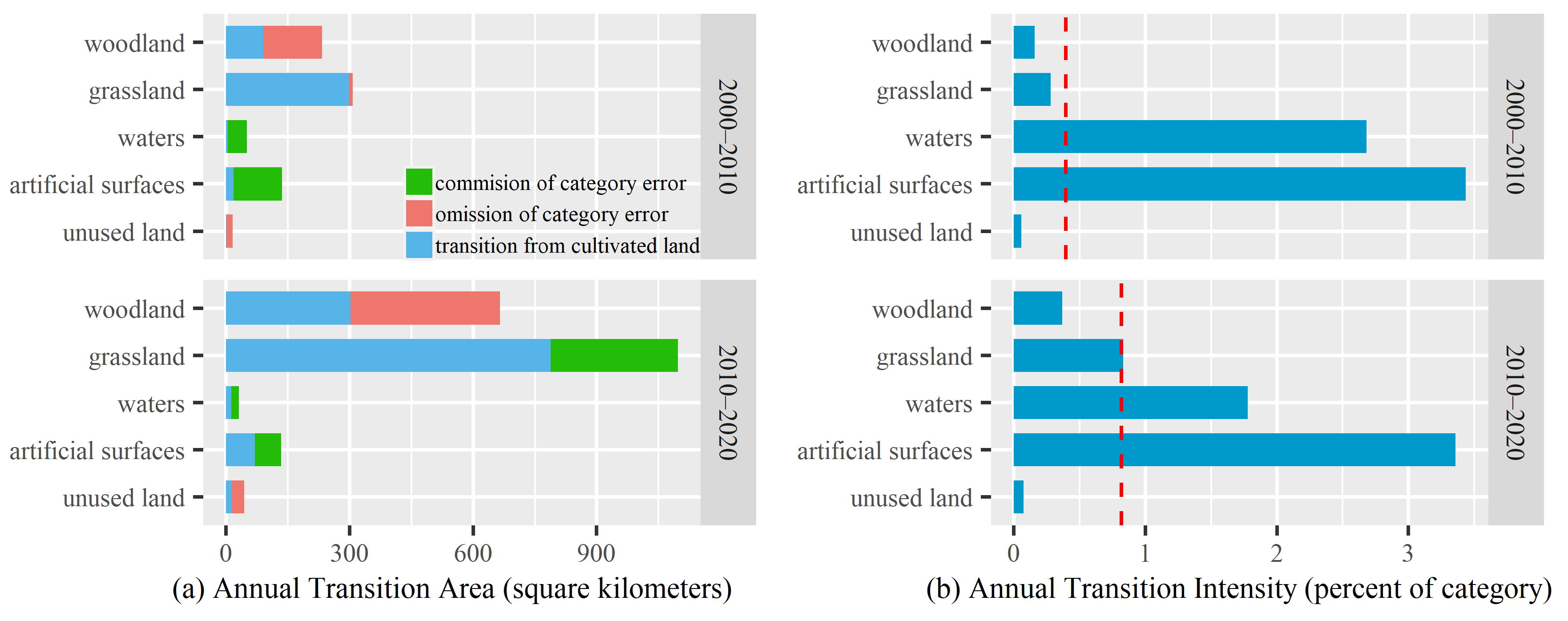
3.3. Transition Level

Considering the rapid urbanization and increased human activities, this study focused on the transition to artificial surfaces and cultivated land from other LULC types. The transition from cultivated land, woodland, grassland, waters, unused land to artificial surfaces in the upper reaches of the YRB is shown in Figure 13. Figure 13a indicates the transition size along with hypothetical errors in the LULC data at the initial year that could account for the difference between transition intensity and the uniform intensity line for the upper reaches. Figure 13b shows the transition intensity. If the bar ends before the uniform intensity line, then the gain of artificial surfaces avoids the corresponding category. On the other hand, if the bar extends beyond the uniform intensity line, then the gain of artificial surfaces targets that category. Gains in artificial surfaces targeted cultivated land and avoided the other four land use types during the two time intervals in the upper and middle reaches (Figure 13 and Figure 14). For the lower reaches, the gains in artificial surfaces targeted both the cultivated land and unused land (Figure 15). The uniform transition and the errors in the initial years of the time intervals that can account for the departures from uniform transition intensity are shown in Figure 13a, Figure 14a, Figure 15a, Figure 16a, Figure 17a and Figure 18a.

The transitions from cultivated land to woodland, grassland, and other land use types in the upper and middle reaches of the YRB are shown in Figure 16 and Figure 17, respectively. The loss of cultivated land targeted grassland and artificial surfaces more intensively than other categories in the upper reaches. Whereas in the middle reaches, the annual transition sizes from cultivated land to grassland and woodland were larger than the other categories (Figure 17a). The hypothetical error in the land use data for 2000, which accounts for the divergences from the uniform intensity for the period of 2000–2010, and the hypothetical error in the LULC data for 2010, which accounts for the divergences from the uniform intensity for the period 2010–2020 are shown in Figure 16a or Figure 17a. For the upper reaches, a transition error of 67.5% in the data for 2000 can account for the deviations from the uniform intensity given the cultivated land loss during 2000–2010. Transition errors in 59% of the 2010 data can account for the deviations from uniform intensity given cultivated land loss during 2010–2020. Whereas for the middle reaches, the corresponding values were 67.0% of the 2000 LULC data and 52.0% of the 2010 LULC data.

The transition intensities of cultivated land gains from other LULC types in the lower reaches of the YRB are shown in Figure 18. The gain of cultivated land targeted artificial surfaces during 2000–2010 and targeted unused land during 2010–2020 most intensively in the lower reaches. Transition errors in 56.2% of the 2000 data can account for the deviations from uniform intensity given cultivated land gain during 2000–2010. Transition errors in 48.6% of the 2010 data can account for the deviations from uniform intensity given cultivated land gain during 2010–2020.

4. Discussion

For all of the three reaches of the YRB, the total land change rate of the second period was faster than the first period. The values of the uniform change intensity for 2010–2020 were 1.40, 2.65, and 1.36 times higher than for the period 2000–2010 for the upper, middle, and lower reaches, respectively. For the middle reaches, the uniform change intensity during the second period was almost three times higher than during the first period. There are several reasons for the differences in the uniform change intensity in region and time. First, there were obvious territorial disparities between the upper, middle, and lower YRB. The economic development of the middle reaches lagged behind that of the lower reaches, which led to the slower land transitions in the earlier period and the greater land transitions in the latter period. Second, the land resources of the middle reaches were much richer than the lower reaches, and the contradictions between artificial surfaces, cultivated land, and ecological land were relatively moderate. Accordingly, the restrictions on land use transition were looser than the lower reaches. Third, some ecological restoration and land consolidation projects have been carried out over the last decades. For example, several provinces in the middle reaches such as Shanxi, Inner Mongolia, and Shaanxi have launched the reclamation of abandoned industrial and mining areas from 2012, which contributed to the land transitions in the middle reaches.

In all three reaches, the largest quantity component of change was for artificial surfaces gain in terms of intensity. Whereas in terms of size, the largest quantity components of change were for cultivated land loss in the middle and lower reaches, and for grassland loss in the upper reaches. The temporal land change rate of the upper reaches was slower than the lower and middle reaches. The results are in line with the background of economic development and urbanization in China [46].

The gross changes were 3.6, 6.3, and 2.4 times larger than the net changes in the upper reaches, middle reaches, and lower reaches, respectively. The exchange component was the largest, which is in line with Sbafizadeh-Moghadam et al. [17], who found that the exchange component accounted for three quarters of the overall temporal change during 2000–2010 in Asia based on the GlobeLand30 data in 2000 and 2010. Sohl et al. [47] assessed the modeled LULC and the existing data sources for the conterminous United States, and they found that the exchange component was the largest component of difference between the modeled and the existing LULC data. Cissell et al. [48] mapped and quantified mangrove forest cover changes along Campeche’s coast from 1999 to 2016, and the results showed that the exchange component was the largest overall for the land use change in their study. In addition, some studies analyzed the quantity and allocation components, without further dividing the allocation component into exchange and shift components [49].

The programs, such as the large-scale development strategy for the western region, put forward the expansion of artificial surfaces in the YRB. As a result, artificial surfaces were the most intensively active category during 2000–2010 for the three reaches. The increase in the artificial surface led to the occupation of cultivated land and ecological land. Cultivated land continued to be lost for all three reaches during the two intervals, which was caused by rapid industrialization and urbanization over the last two decades. In addition, in the upper and middle reaches, another important reason for the cultivated land loss was the Grain to Green Program and the Slope Cropland Control Projects. In the upper and middle reaches, the ecological environment is fragile and soil erosion is severe, and the cultivation conditions are relatively poor. Therefore, ecological restoration projects such as the Grain to Green Program were implemented from 2000, which aim to return cultivated land to forest and grassland in the ecologically vulnerable areas. As Figure 17 shows, the transition size from cultivated land to grassland and woodland was larger than other categories in the middle reaches, which provides evidence for the effects of the Grain to Green Program. Figure 4 also shows that the woodland area increased most intensively among all of the categories during 2000–2010, which was an achievement of the ecological project.

Although ecological restoration programs have been carried out for almost 20 years, our results still find that the net area of grassland in the upper and middle reaches kept reducing during 2000–2020. This was different from the results from Zhang et al. [19], who found that the area of grassland increased from 2000–2018 markedly. The reason may be that the land use data set used in Zhang et al. and in this study are different. The GlobeLand30 data set with a 30 × 30 m² spatial resolution was used in this study, while Zhang et al. used another land use data set with a 1 × 1 km² spatial resolution [50]. In addition, some grassland was transferred to woodland with the implementation of the projects of Construction of Windblown Sand Protection Forest [51]. Furthermore, the effectiveness of ecological restoration programs in protecting vegetation land is uncertain in some regions. Jiang et al. [52] found that the soil erosion for the northern dryland of China was substantially reduced; however, the vegetation cover presented decreasing trends significantly in certain sandstorm regions. In these areas, several drought events restrained plant growth and, finally, offset afforestation measures to some extent since 2005. Therefore, identifying suitable time and environmental conditions for implementing ecological restoration programs is critical to achieving targets.

A large amount of high-quality cultivated land is distributed in the lower reaches of the YRB such as in Shandong Province and Hunan Province. The occupation of cultivated land by artificial surfaces would threaten food security. Therefore, the cultivated land Red Line and Requisition Compensation Balance policy was put forward. According to the policies, the losses in cultivated land to artificial surfaces should be replenished with new cultivated land elsewhere, aiming for a constant area of cultivated land in the long term [53]. These cultivated land protection policies were implemented strictly in the provinces of the lower reaches, since these provinces have high-quality cultivated land and are important agricultural supply areas. As Figure 18 shows, the gain in cultivated land targeted unused land mostly in terms of size and intensity. In the lower reaches of the YRB, the unused land was mainly bare land with vegetation cover lower than 10%, including desert, sandy fields, Gobi, bare rocks, saline, and alkaline land, etc. [44]. Therefore, it is important to pay attention to the quality of the new cultivated land that is used to supplement the quantity of cultivated land. The policy aim should be quality equilibrium instead of just quantity equilibrium.

In the upper reaches, the woodland commission hypothetical error was larger than the other errors during 2000–2010, and the artificial surfaces commission hypothesis error was largest during 2010–2020. Therefore, there was powerful evidence for the conclusion of active gain in woodland during 2000–2010 and active gain in artificial surfaces during 2010–2020. During 2000–2010, grassland commission error in the middle reaches was lower; therefore, the evidence for active grassland loss was weak. Similarly, in the middle reaches, the cultivated land omission error was largest, so there was powerful evidence for the conclusion that cultivated land was dormant regarding gains rather than the other conclusion with respect to gains. In the lower reaches, the artificial surfaces commission and cultivated land omission hypothetical errors were larger; therefore, there was powerful evidence that artificial surfaces gain was active and cultivated land gain was dormant.

5. Conclusions

The application of an intensity analysis framework to GlobeLand30 data of the YRB revealed the size and intensity of LULC changes in this study. The results showed that the overall LULC change in the three reaches of the YRB has been accelerating, reflecting the socioeconomic development of this region during 2000–2020. The increase in the uniform land change intensity was especially large for the middle reaches, owing to the factors of territorial characteristics, land resource enrichment, and environmental projects. The exchange component was the largest overall for each of the reaches during both time intervals, and this result was consistent with several previous studies worldwide. The upper reaches are the environmentally fragile zone, and ecological projects have been carried out since 2000. As a result, the woodland experienced the largest gain intensity during 2000–2010. For the middle reaches, grassland and cultivated land had the largest gains and losses, but cultivated land was dormant during the two intervals owing to the large area it covers. The land resource in the lower reaches is mostly limited, and the contradiction between the artificial surfaces and cultivated land is outstanding. The new cultivated land was mainly transferred from artificial and unused lands under the Requisition–Compensation Balance policy. The size of the minimum hypothetical errors indicated the strength of the evidence for the deviation from the uniform intensity. Based on this research, the causal relationship between LULC change and the potential driving factors for the YRB will be examined quantitatively using statistical methods and machine learning in the future.

References

1. Da, F.; Chen, X.; Qi, J. Spatiotemporal Characteristic of Land Use/Land Cover Changes in the Middle and Lower Reaches of Shule River Basin Based on an Intensity Analysis. Sustainability 2019, 11, 1360. [Google Scholar] [CrossRef] [Green Version]
2. Malek, Ž.; Verburg, P. Mapping global patterns of land use decision-making. Glob. Environ. Change 2020, 65, 102170. [Google Scholar] [CrossRef]
3. Munch, Z. Global and local patterns of landscape change accuracy. ISPRS J. Photogramm. Remote Sens. 2020, 161, 264–277. [Google Scholar] [CrossRef]
4. Aldwaik, S.Z.; Pontius, R.G. Intensity analysis to unify measurements of size and stationarity of land changes by interval, category, and transition. Landsc. Urb. Plan. 2012, 106, 103–114. [Google Scholar] [CrossRef]
5. Pontius, R.G.; Gao, Y.; Giner, N.M.; Kohyama, T.; Osaki, M.; Hirose, K. Design and Interpretation of Intensity Analysis Illustrated by Land Change in Central Kalimantan, Indonesia. Land 2013, 2, 351–369. [Google Scholar] [CrossRef]
6. Tankpa, V.; Wang, L.; Atanga, R.A.; Awotwi, A.; Guo, X. Evidence and impact of map error on land use and land cover dynamics in Ashi River watershed using intensity analysis. PLoS ONE 2020, 15. [Google Scholar] [CrossRef] [Green Version]
7. Akinyemi, F.O.; Pontius, R.G., Jr.; Braimoh, A.K. Land change dynamics: Insights from Intensity Analysis applied to an African emerging city. J. Sp. Sci. 2017, 62, 69–83. [Google Scholar] [CrossRef]
8. Akodéwou, A.; Oszwald, J.; Gazull, L.; Akpavi, S.; Koffi, A.; Gond, V.; Saidi, S. Land Use and Land Cover Dynamics Analysis of the Togodo Protected Area and Its Surroundings in Southeastern Togo, West Africa. Sustainability 2020, 12, 5439. [Google Scholar] [CrossRef]
9. Anteneh, Y.; Stellmacher, T.; Zeleke, G.; Mekuria, W.; Gebremariam, E. Dynamics of land change: Insights from a three-level intensity analysis of the Legedadie-Dire catchments, Ethiopia. Environ. Monit. Assess. 2018, 190. [Google Scholar] [CrossRef]
10. Feng, Y.; Lei, Z.; Tong, X.; Gao, C.; Chen, S.; Wang, J.; Wang, S. Spatially-explicit modeling and intensity analysis of China’s land use change 2000-2050. J. Environ. Manag. 2020, 263. [Google Scholar] [CrossRef]
11. Nyamekye, C.; Kwofie, S.; Ghansah, B.; Agyapong, E.; Boamah, L.A. Assessing urban growth in Ghana using machine learning and intensity analysis: A case study of the New Juaben Municipality. Land Use Policy 2020, 99, 105057. [Google Scholar] [CrossRef]
12. Sun, X.; Yu, C.; Wang, J.; Wang, M. The Intensity Analysis of Production Living Ecological Land in Shandong Province, China. Sustainability 2020, 12, 8326. [Google Scholar] [CrossRef]
13. Niya, A.K.; Huang, J.; Karimi, H.; Keshtkar, H.; Naimi, B. Use of Intensity Analysis to Characterize Land Use/Cover Change in the Biggest Island of Persian Gulf, Qeshm Island, Iran. Sustainability 2019, 11, 4396. [Google Scholar] [CrossRef] [Green Version]
14. Ekumah, B.; Armah, F.A.; Afrifa, E.K.A.; Aheto, D.W.; Odoi, J.O.; Afitiri, A.-R. Assessing land use and land cover change in coastal urban wetlands of international importance in Ghana using Intensity Analysis. Wetl. Ecol. Manag. 2020, 28, 271–284. [Google Scholar] [CrossRef]
15. Mwangi, H.M.; Lariu, P.; Julich, S.; Patil, S.D.; McDonald, M.A.; Feger, K.-H. Characterizing the Intensity and Dynamics of Land-Use Change in the Mara River Basin, East Africa. Forests 2018, 9, 8. [Google Scholar] [CrossRef] [Green Version]
16. Quan, B.; Pontius, R.G., Jr.; Song, H. Intensity Analysis to communicate land change during three time intervals in two regions of Quanzhou City, China. Gisci. Remote Sens. 2020, 57, 21–36. [Google Scholar] [CrossRef]
17. Sbafizadeh-Moghadam, H.; Minaei, M.; Feng, Y.; Pontiu, R.G., Jr. GlobeLand30 maps show four times larger gross than net land change from 2000 to 2010 in Asia. Int. J. Appl. Earth Obs. Geoinf. 2019, 78, 240–248. [Google Scholar] [CrossRef]
18. Pontius, R.G., Jr.; Santacruz, A. Quantity, exchange, and shift components of difference in a square contingency table. Int. J. Remote Sens. 2014, 35, 7543–7554. [Google Scholar] [CrossRef]
19. Zhang, W.; Lu, X.; Shi, Y.; Sun, P.; Zhang, Y. Graphic Characteristics of Land Use Transition in the Yellow River Basin. China Land Sci. 2020, 34, 80–88. [Google Scholar]
20. Aldwaik, S.Z.; Pontius, R.G., Jr. Map errors that could account for deviations from a uniform intensity of land change. Int. J. Geogr. Inf. Sci. 2013, 27, 1717–1739. [Google Scholar] [CrossRef]
21. Xie, Z.; Pontius, R.G., Jr.; Huang, J.; Nitivattananon, V. Enhanced Intensity Analysis to Quantify Categorical Change and to Identify Suspicious Land Transitions: A Case Study of Nanchang, China. Remote Sens. 2020, 12, 3323. [Google Scholar] [CrossRef]
22. Xiao, D.; Niu, H.; Yan, H.; Fan, L.; Zhao, S. Spatiotemperal evolution of land use pattern in the Yellow River Basin (Henan section) from 1990 to 2018. Trans. Chin. Soc. Agric. Eng. 2020, 36, 271–281. [Google Scholar]
23. Zhang, R.; Wang, Y.; Chang, J.; Li, Y. Response of land use change to human activities in the Yellow River Basin based on water resources division. J. Nat. Resour. 2019, 34, 274–287. [Google Scholar]
24. Liu, J.; Kuang, W.; Zhang, Z.; Xu, X.; Qin, Y.; Ning, J.; Zhou, W.; Zhang, S.; Li, R.; Yan, C.; et al. Spatiotemporal characteristics, patterns, and causes of land-use changes in China since the late 1980s. J. Geogr. Sci. 2014, 24, 195–210. [Google Scholar] [CrossRef]
25. Liu, J.; Zhang, Z.; Xu, X.; Kuang, W.; Zhou, W.; Zhang, S.; Li, R.; Yan, C.; Yu, D.; Wu, S.; et al. Spatial patterns and driving forces of land use change in China during the early 21st century. J. Geogr. Sci. 2010, 20, 483–494. [Google Scholar] [CrossRef]
26. Jun, C.; Ban, Y.; Li, S. Open access to Earth land-cover map. Nature 2014, 514, 434. [Google Scholar] [CrossRef] [Green Version]
27. Arsanjani, J.J. Characterizing and monitoring global landscapes using GlobeLand30 datasets: The first decade of the twenty-first century. Int. J. Digit. Earth 2019, 12, 642–660. [Google Scholar] [CrossRef]
28. Gong, P.; Liu, H.; Zhang, M.; Li, C.; Wang, J.; Huang, H.; Clinton, N.; Ji, L.; Li, W.; Bai, Y.; et al. Stable classification with limited sample: Transferring a 30-m resolution sample set collected in 2015 to mapping 10-m resolution global land cover in 2017. Sci. Bull. 2019, 64, 370–373. [Google Scholar] [CrossRef] [Green Version]
29. Grekousis, G.; Mountrakis, G.; Kavouras, M. An overview of 21 global and 43 regional land-cover mapping products. Int. J. Remote Sens. 2015, 36, 5309–5335. [Google Scholar] [CrossRef]
30. Hu, Q.; Xiang, M.; Chen, D.; Zhou, J.; Wu, W.; Song, Q. Global cropland intensification surpassed expansion between 2000 and 2010: A spatio-temporal analysis based on GlobeLand30. Sci. Total Environ. 2020, 746. [Google Scholar] [CrossRef]
31. Arsanjani, J.J.; See, L.; Tayyebi, A. Assessing the suitability of GlobeLand30 for mapping land cover in Germany. Int. J. Digit. Earth 2016, 9, 873–891. [Google Scholar] [CrossRef] [Green Version]
32. Arsanjani, J.J.; Tayyebi, A.; Vaz, E. GlobeLand30 as an alternative fine-scale global land cover map: Challenges, possibilities, and implications for developing countries. Habitat Int. 2016, 55, 25–31. [Google Scholar] [CrossRef]
33. Balogun, A.-L.; Said, S.A.M.; Sholagberu, A.T.; Aina, Y.A.; Althuwaynee, O.F.; Aydda, A. Assessing the suitability of GlobeLand30 for land cover mapping and sustainable development in Malaysia using error matrix and unbiased area Estimation. Geocarto Int. 2020, 1–21. [Google Scholar] [CrossRef]
34. Wang, Y.; Zhang, J.; Liu, D.; Yang, W.; Zhang, W. Accuracy Assessment of GlobeLand30 2010 Land Cover over China Based on Geographically and Categorically Stratified Validation Sample Data. Remote Sens. 2018, 10, 1213. [Google Scholar] [CrossRef] [Green Version]
35. Pan, H.; Tong, X.; Xu, X.; Luo, X.; Jin, Y.; Xie, H.; Li, B. Updating of Land Cover Maps and Change Analysis Using GlobeLand30 Product: A Case Study in Shanghai Metropolitan Area, China. Remote Sens. 2020, 12, 3147. [Google Scholar] [CrossRef]
36. Shi, L.; Cai, Z.; Ding, X.; Di, R.; Xiao, Q. What Factors Affect the Level of Green Urbanization in the Yellow River Basin in the Context of New-Type Urbanization? Sustainability 2020, 12, 2488. [Google Scholar] [CrossRef] [Green Version]
37. Chen, Y.P.; Fu, B.J.; Zhao, Y.; Wang, K.B.; Zhao, M.M.; Ma, J.F.; Wu, J.H.; Xu, C.; Liu, W.G.; Wang, H. Sustainable development in the Yellow River Basin: Issues and strategies. J. Clean. Prod. 2020, 263. [Google Scholar] [CrossRef]
38. Xu, S.; Yu, Z.; Yang, C.; Ji, X.; Zhang, K. Trends in evapotranspiration and their responses to climate change and vegetation greening over the upper reaches of the Yellow River Basin. Agric. Forest Meteorol. 2018, 263, 118–129. [Google Scholar] [CrossRef]
39. Lu, X.; Qu, Y.; Sun, P.; Yu, W.; Peng, W. Green Transition of Cultivated Land Use in the Yellow River Basin: A Perspective of Green Utilization Efficiency Evaluation. Land 2020, 9, 475. [Google Scholar] [CrossRef]
40. Zhang, W.; Wang, L.; Xiang, F.; Qin, W.; Jiang, W. Vegetation dynamics and the relations with climate change at multiple time scales in the Yangtze River and Yellow River Basin, China. Ecol. Indic. 2020, 110. [Google Scholar] [CrossRef]
41. Yuan, M.; Zhao, L.; Lin, A.; Li, Q.; She, D.; Qu, S. How do climatic and non-climatic factors contribute to the dynamics of vegetation autumn phenology in the Yellow River Basin, China? Ecol. Indic. 2020, 112. [Google Scholar] [CrossRef]
42. Omer, A.; Ma, Z.; Zheng, Z.; Saleem, F. Natural and anthropogenic influences on the recent droughts in Yellow River Basin, China. Sci. Total Environ. 2020, 704. [Google Scholar] [CrossRef]
43. Chen, J.; Chen, J.; Liao, A.; Cao, X.; Chen, L.; Chen, X.; He, C.; Han, G.; Peng, S.; Lu, M.; et al. Global land cover mapping at 30 m resolution: A POK-based operational approach. ISPRS J. Photogramm. Remote Sens 2015, 103, 7–27. [Google Scholar] [CrossRef] [Green Version]
44. Chen, J.; Cao, X.; Peng, S.; Ren, H. Analysis and Applications of GlobeLand30: A Review. ISPRS Int. J. Geo-Inf. 2017, 6, 230. [Google Scholar]
45. Pontius, R.G., Jr. Component intensities to relate difference by category with difference overall. Int. J. Appl. Earth Obs. Geoinform. 2019, 77, 94–99. [Google Scholar] [CrossRef]
46. Wang, F.; An, L.; Dang, A.; Han, J.; Miao, C.; Wang, J.; Zhang, G.; Zhao, Y. Human-land coupling and sustainable human settlements in the Yellow River Basin. Geogr. Res. 2020, 39, 1707–1724. [Google Scholar]
47. Sohl, T.; Reker, R.; Bouchard, M.; Sayler, K.; Dornbierer, J.; Wika, S.; Quenzer, R.; Friesz, A. Modeled historical land use and land cover for the conterminous United States. J. Land Use Sci. 2016, 11, 476–499. [Google Scholar] [CrossRef]
48. Cissell, J.R.; Delgado, A.M.; Sweetman, B.M.; Steinberg, M.K. Monitoring mangrove forest dynamics in Campeche, Mexico, using Landsat satellite data. Remote Sens. Appl. Soc. Environ. 2018, 9, 60–68. [Google Scholar] [CrossRef]
49. Malek, Ž.; Verburg, P. Mediterranean land systems: Representing diversity and intensity of complex land systems in a dynamic region. Lands. Urb. Plan. 2017, 165, 102–116. [Google Scholar] [CrossRef] [Green Version]
50. Ning, J.; Liu, J.; Kuang, W.; Xu, X.; Zhang, S.; Yan, C.; Li, R.; Wu, S.; Hu, Y.; Du, G.; et al. Spatiotemporal patterns and characteristics of land-use change in China during 2010–2015. J. Geogr. Sci. 2018, 28, 547–562. [Google Scholar] [CrossRef] [Green Version]
51. Mao, D.; Wang, Z.; Wu, B.; Zeng, Y.; Luo, L.; Zhang, B. Land degradation and restoration in the arid and semiarid zones of China: Quantified evidence and implications from satellites. Land Degrad. Dev. 2018, 29, 3841–3851. [Google Scholar] [CrossRef]
52. Jiang, C.; Zhang, H.; Zhao, L.; Yang, Z.; Wang, X.; Yang, L.; Wen, M.; Geng, S.; Zeng, Q.; Wang, J. Unfolding the effectiveness of ecological restoration programs in combating land degradation: Achievements, causes, and implications. Sci. Total Environ. 2020, 748, 141552. [Google Scholar] [CrossRef] [PubMed]
53. Wang, M.; Sun, X.; Fan, Z.; Yue, T. Investigation of Future Land Use Change and Implications for Cropland Quality: The Case of China. Sustainability 2019, 11, 3327. [Google Scholar] [CrossRef] [Green Version]
Figure 1. The location of Yellow River Basin (YRB) (a), land use and land cover (LULC) patterns in 2000 (b), 2010 (c), and 2020 (d).
Land 10 00031 g001
Figure 2. Schematic representation of the main methods followed in this study.
Land 10 00031 g002
Figure 3. Size of interval level changes for the upper, middle, and lower reaches during the two time intervals (T1: 2000–2010, T2: 2010–2020). (a) Interval change area along with the hypothetical errors; (b) interval change component in terms of intensity.
Land 10 00031 g003
Figure 4. Category level gain and loss intensities through two time intervals for the upper reaches of the YRB. The red vertical dashed line is the uniform intensity line.
Land 10 00031 g004
Figure 5. Category level change sizes along with hypothetical errors for the upper reaches of the YRB. (a) 2000–2010; (b) 2010–2020.
Land 10 00031 g005
Figure 6. Category level gain and loss intensities through two time intervals for the middle reaches of the YRB.
Land 10 00031 g006
Figure 7. Category level change sizes along with hypothetical errors for the middle reaches of the YRB.
Land 10 00031 g007
Figure 8. Category level gain and loss intensities through two time intervals for the lower reaches of the YRB. (a), 2000–2010; (b) 2010–2020.
Land 10 00031 g008
Figure 9. Category level change sizes along with hypothetical errors for the lower reaches of the YRB.
Land 10 00031 g009
Figure 10. Size (a) and Intensity (b) of differences for upper reaches of the YRB. The sign “+” denotes net gain and the sign “−” denotes net loss.
Land 10 00031 g010
Figure 11. Size (a) and Intensity (b) of differences for the middle reaches of the YRB. The sign “+” denotes net gain and the sign “−” denotes net loss.
Land 10 00031 g011
Figure 12. Size (a) and Intensity (b) of differences for the lower reaches of the YRB. The sign “+” denotes net gain and the sign “−” denotes net loss.
Land 10 00031 g012
Figure 13. Intensity analysis for transition to artificial surfaces for the upper reaches. The transition size along with hypothetical map errors (a); transition intensities (b). The red, vertical dashed lines indicate the uniform intensities.
Land 10 00031 g013
Figure 14. Intensity analysis for transition to artificial surfaces for the middle reaches. The transition size along with hypothetical map errors (a); transition intensities (b). The red, vertical dashed lines indicate the uniform intensities.
Land 10 00031 g014
Figure 15. Intensity analysis for transition to artificial surfaces for the lower reaches. The transition size along with hypothetical map errors (a); transition intensities (b). The red, vertical dashed lines indicate the uniform intensities.
Land 10 00031 g015
Figure 16. Intensity analysis for cultivated land loss in the upper reaches. The transition size along with hypothetical map errors (a); transition intensities (b). The red, vertical dashed lines indicate the uniform intensities.
Land 10 00031 g016
Figure 17. Intensity analysis for cultivated land loss in the middle reaches. The transition size along with hypothetical map errors (a); transition intensities (b). The red, vertical dashed lines indicate the uniform intensities.
Land 10 00031 g017
Figure 18. Intensity analysis for cultivated land gain in the lower reaches. The transition size along with hypothetical map errors (a); transition intensities (b). The red, vertical dashed lines indicate the uniform intensities.
Land 10 00031 g018
Publisher’s Note: MDPI stays neutral with regard to jurisdictional claims in published maps and institutional affiliations.