Analysis of Changes in Spatio-Temporal Patterns of Drought across South Korea


Abstract
1. Introduction
2. Materials and Methods
2.1. Study Area and Data
2.2. Marginal Distributions and Copulas
2.3. Return Period in a Bivariate Framework
2.4. Kendall Return Period
3. Results
3.1. Drought Characteristics across South Korea during 1980–2015
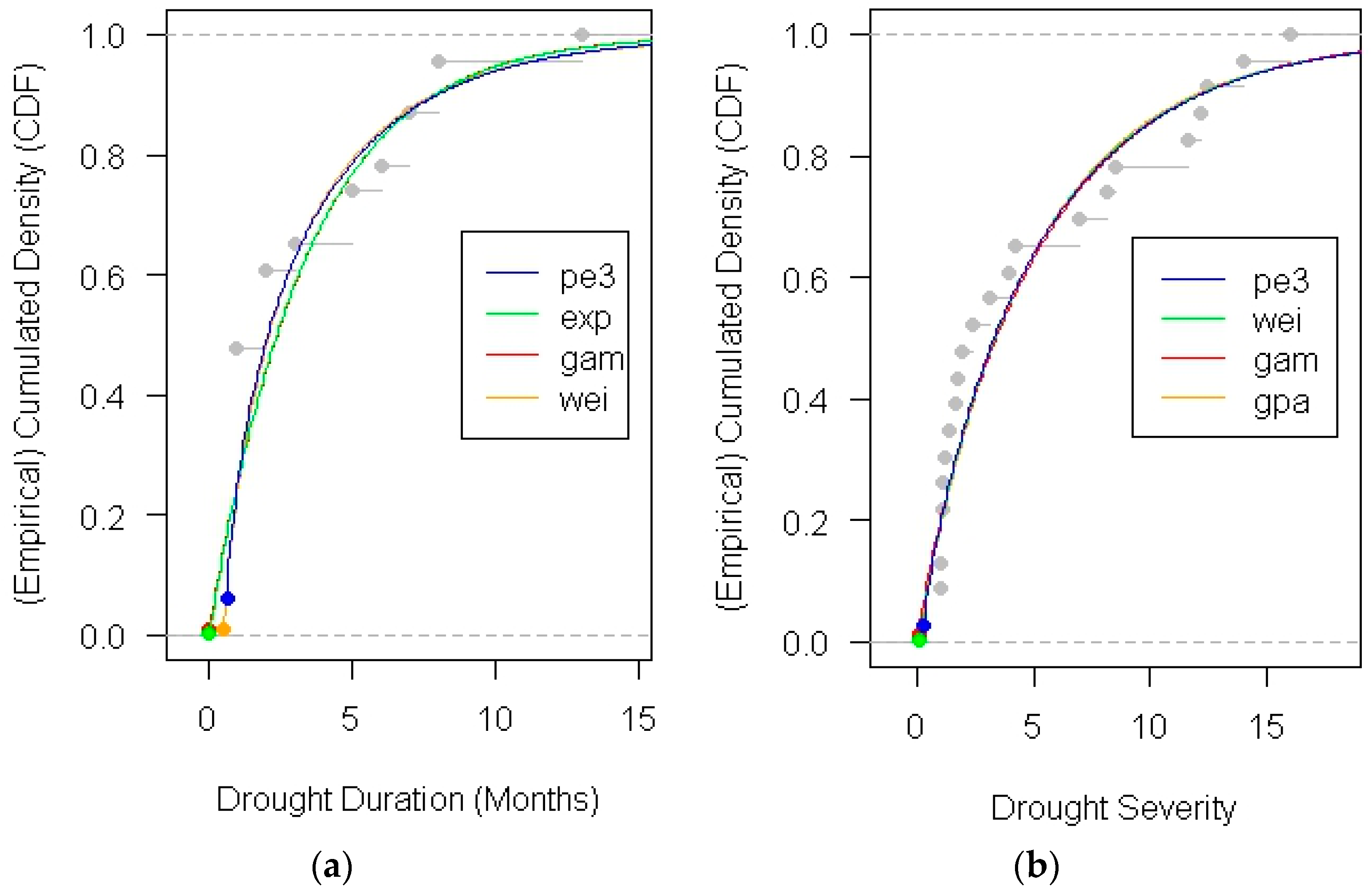
3.2. Marginal Probability Distributions of Drought Duration and Severity
3.3. Application of Bivariate Copulas
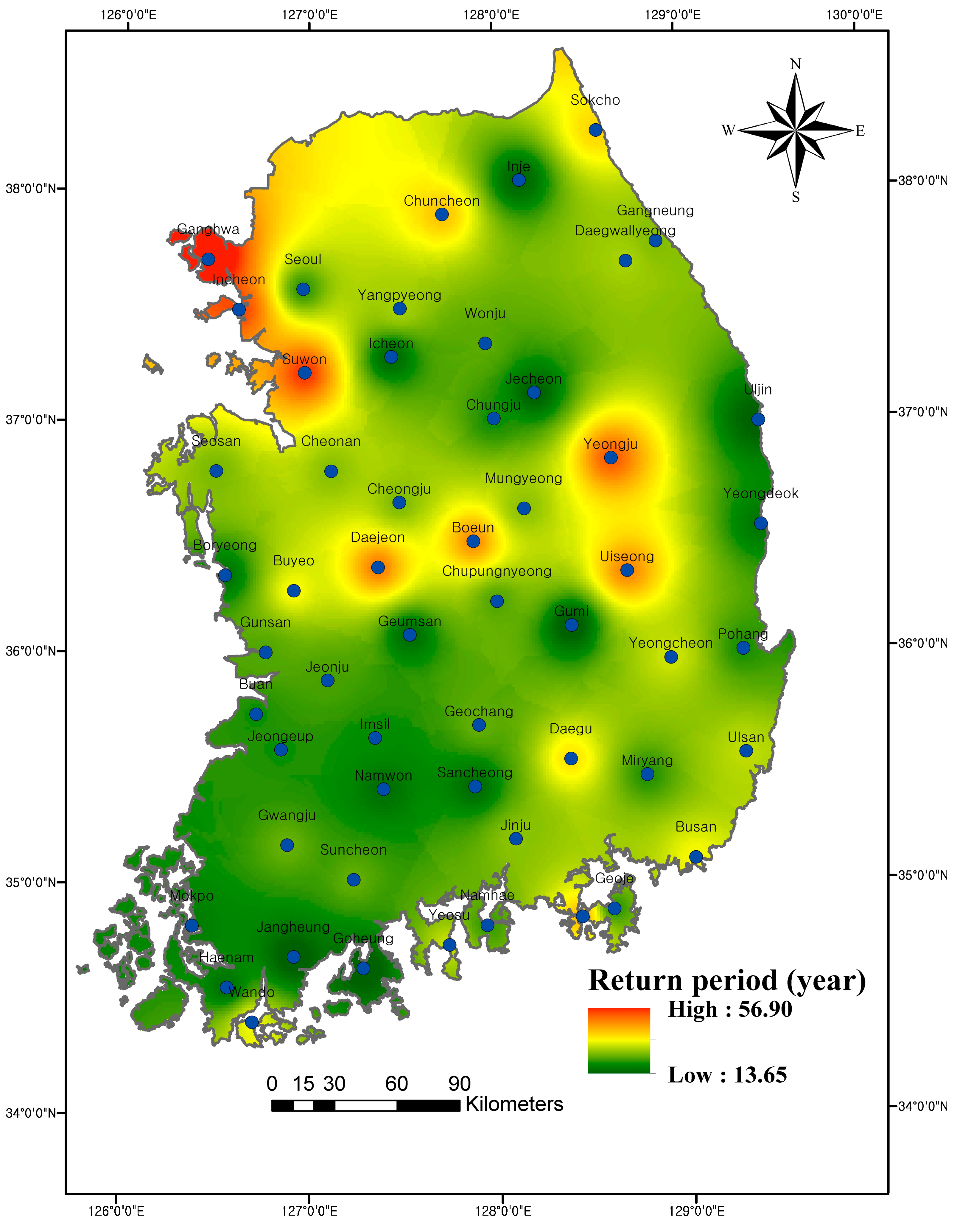
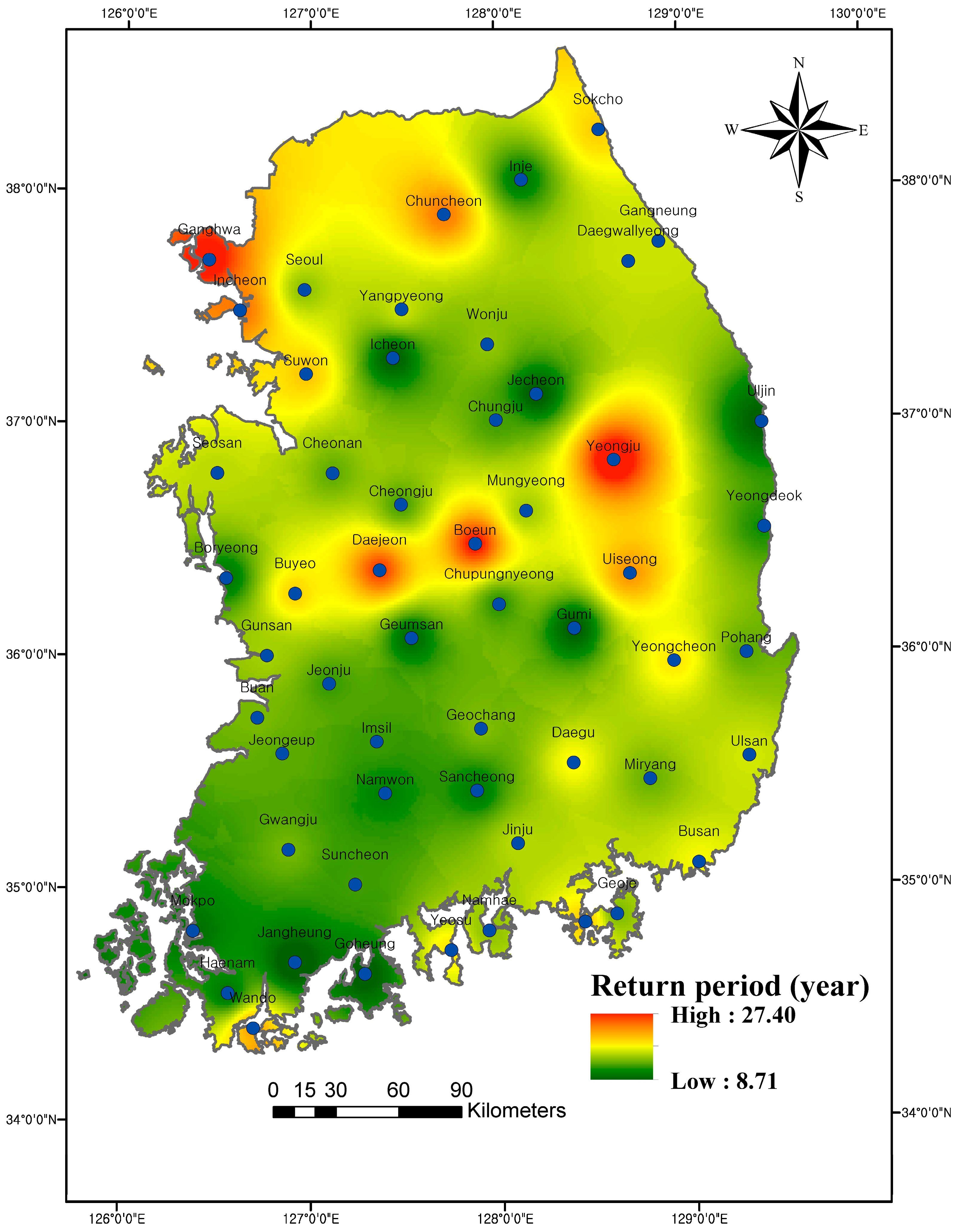
3.4. Spatial Distribution of the Bivariate Return Period
3.5. Comparison of Return Periods Using Identified Drought Events
4. Conclusions
- (1)
- Drought characteristics on the basis of SPI indicate that due to the unusual precipitation pattern in the southwest coastal areas, Jecheon station faced the drought of longest duration and greater severity among 55 stations across South Korea.
- (2)
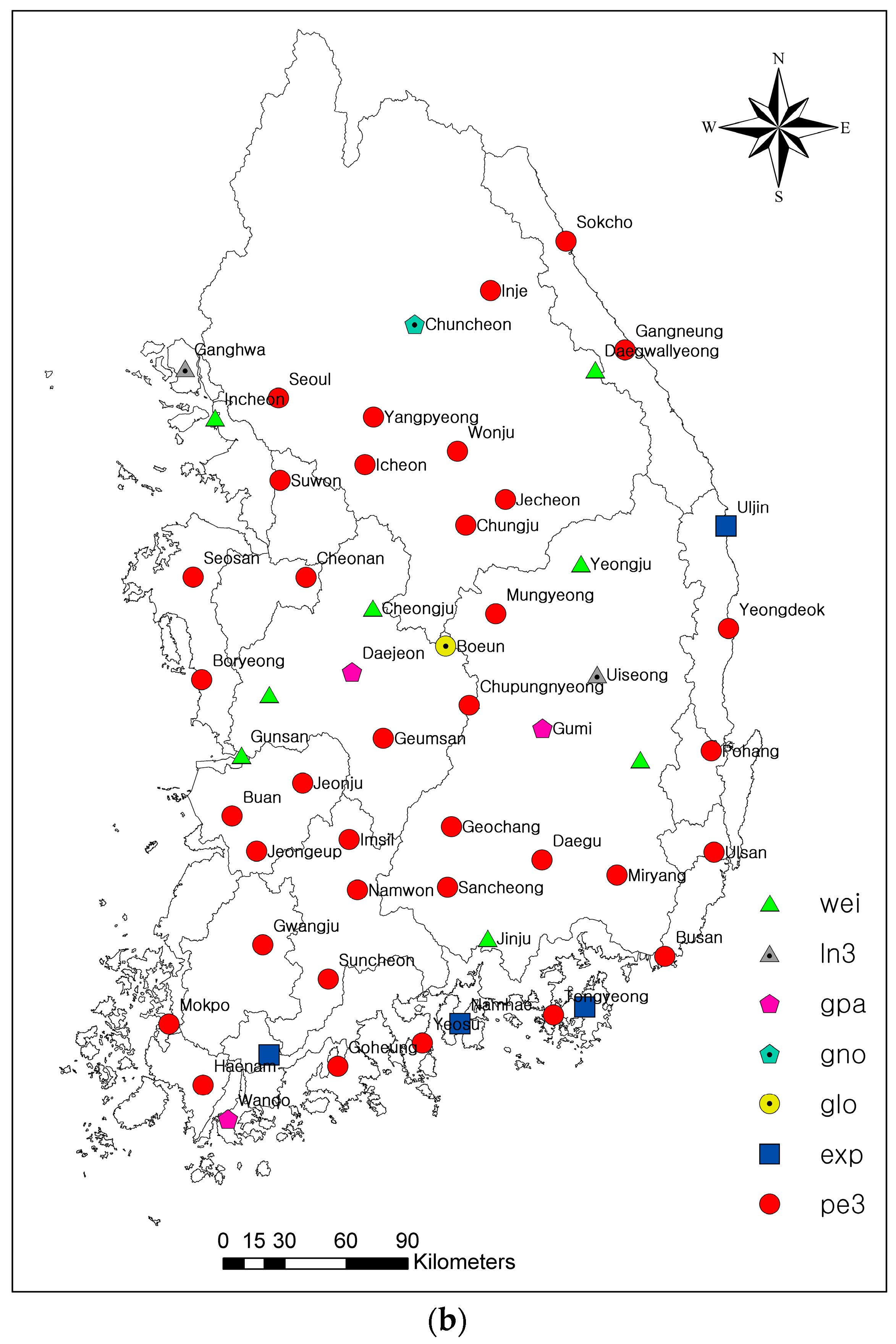
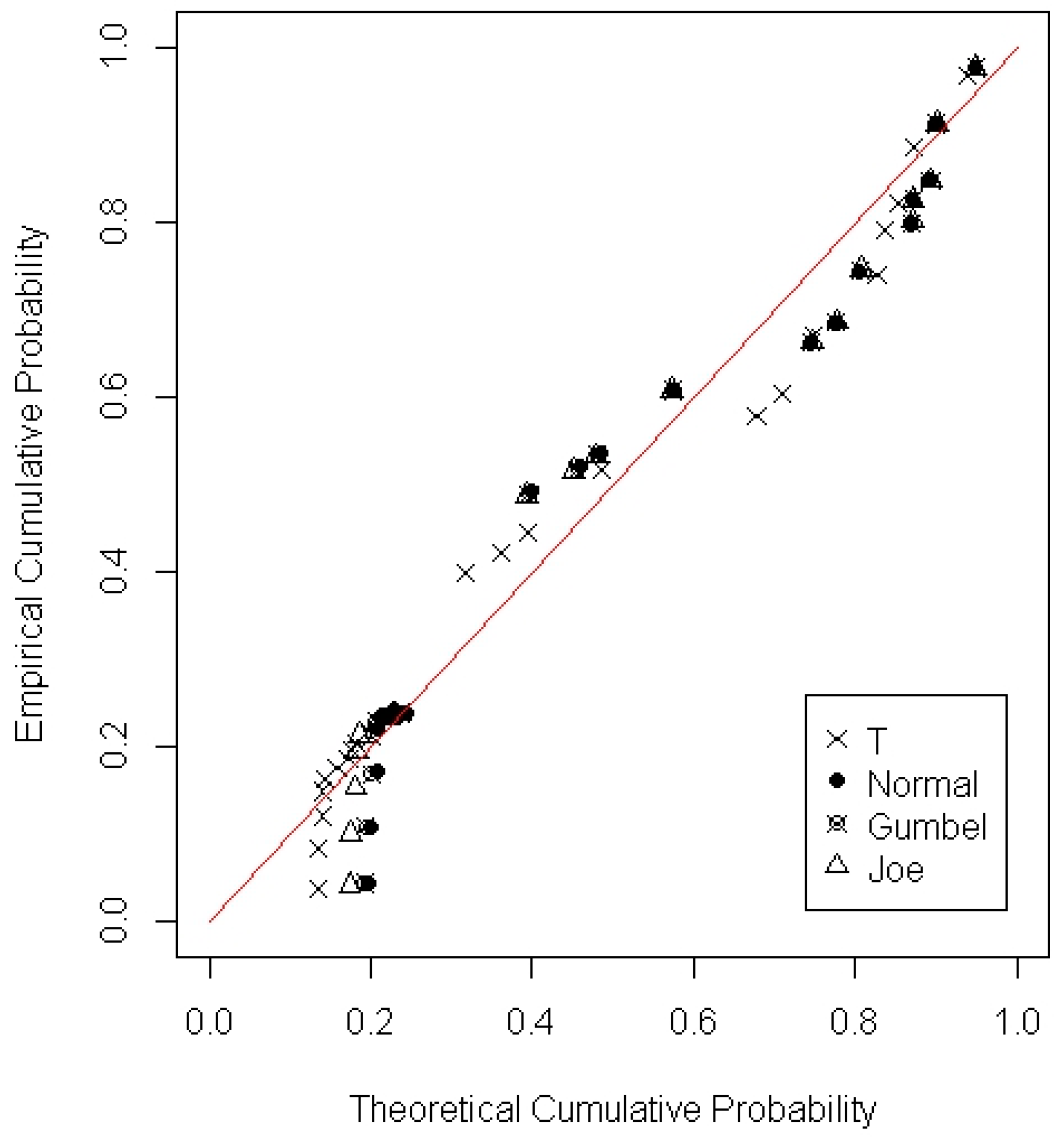
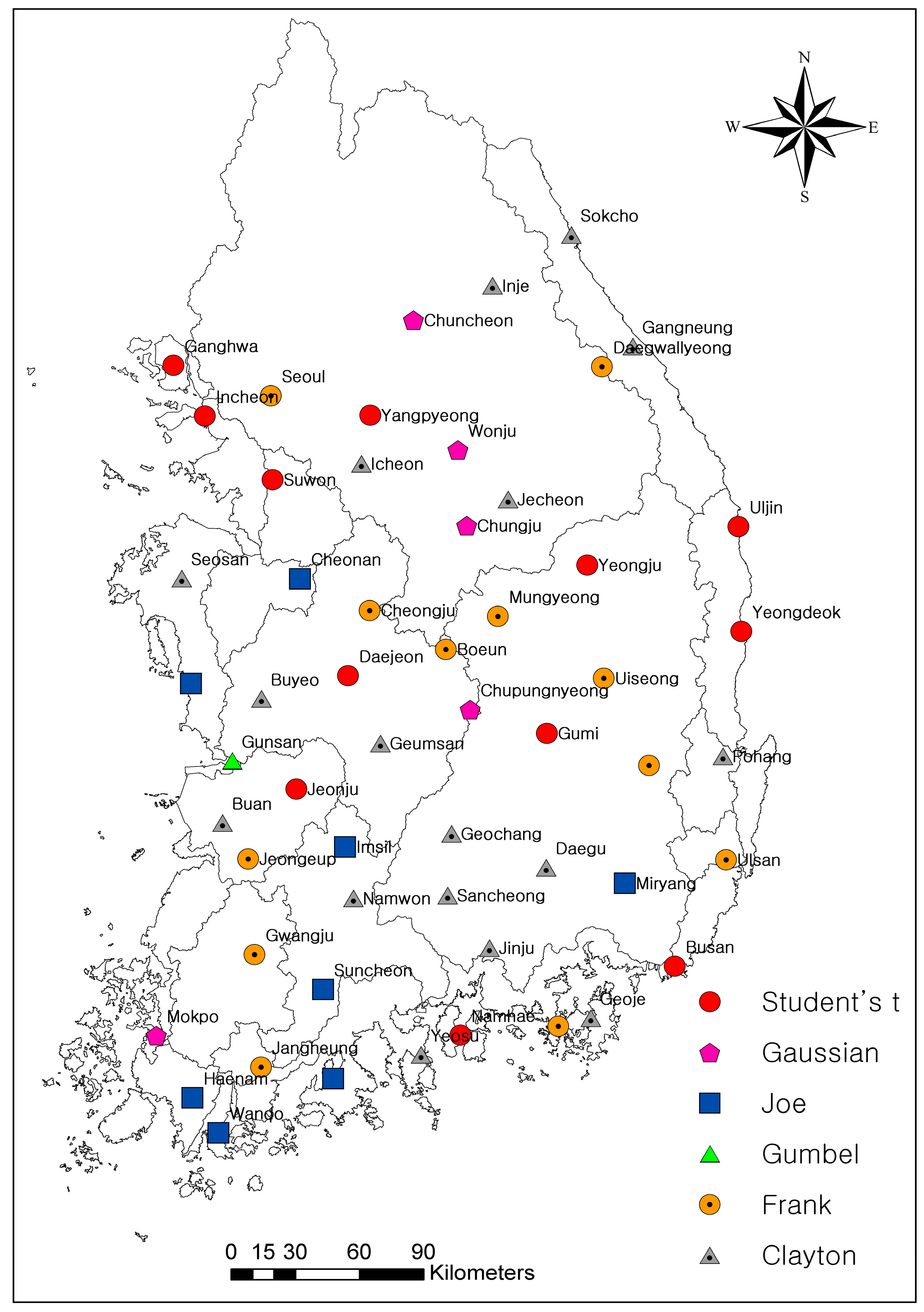
- Based on the KS test, RMSE and graphical comparison applied to 55 stations, four models (exp, wei, gpa and pe3) were best fitted for drought duration and seven models (wei, ln3, gpa, gno, glo, exp, and pe3) for drought severity. Pe3 is the most common model existing in both drought duration and severity. Based on Sn, AIC and the probability-probability plot, the choice of copula varies from station to station. In addition, the Frank copula is the most common best fitted copula among 55 stations. It is concluded that several different measures are necessary to identify the best fit marginal distributions and copulas. Since different measures reflect different characteristics of marginal distributions and copulas, a single measure may lead to under- or over-estimation of the probability of drought.
- (3)
- The properties of the spatial distributions of , and are the same. However, showed droughts of longer durations and higher severities compared to and droughts of shorter durations and lower severities compared to . The spatial distribution of the joint return period indicates that the southwestern coast of South Korea and surrounding areas of Uljin have a high risk of drought, while the northwestern portion and surrounding areas of Yeongju, Uiseong, Boeun and Daejeon stations have a relatively low risk of drought. The results indicate the serious challenge in the water resource management and human mitigation of drought hazards in the southwestern coast due to abrupt changes in the precipitation pattern. In order to cope with drought hazards, accurate hydrological regulations of reservoirs in the southwest coast is necessary.
- (4)
- The comparison of univariate and bivariate return periods using the top twenty drought events showed, as can be noticed from Table 7, that the secondary return period is always larger than the and shorter than . It is also concluded that the Kendall return period and primary return periods cannot be interchanged, as their applicability changes according to the type of drought risk considered.
Acknowledgments
Author Contributions
Conflicts of Interest
References
- Choi, G.; Kwon, W.-T.; Boo, K.-O.; Cha, Y.-M. Recent Spatial and Temporal Changes in Means and Extreme Events of Temperature and Precipitation across the Republic of Korea *. J. Korean Geogr. Soc. 2008, 43, 681–700. [Google Scholar]
- Jo, H.K. Impacts of urban greenspace on offsetting carbon emissions for middle Korea. J. Environ. Manag. 2002, 64, 115–126. [Google Scholar] [CrossRef]
- Boo, K.-O.; Kwon, W.-T.; Oh, J.-H.; Baek, H.-J. Response of global warming on regional climate change over Korea: An experiment with the MM5 model. Geophys. Res. Lett. 2004, 31. [Google Scholar] [CrossRef]
- Lee, J.-H.; Seo, J.-W.; Kim, C.-J. Analysis on Trends, Periodicities and Frequencies of Korean Drought Using Drought Indices. J. Korea Water Resour. Assoc. 2012, 45, 75–89. [Google Scholar] [CrossRef]
- Sawada, Y.; Koike, T.; Jaranilla-Sanchez, P.A. Modeling hydrologic and ecologic responses using a new eco-hydrological model for identification of droughts. Water Resour. Res. 2014, 50, 6214–6235. [Google Scholar] [CrossRef]
- Jaranilla-Sanchez, P.A.; Wang, L.; Koike, T. Modeling the hydrologic responses of the Pampanga River basin, Philippines: A quantitative approach for identifying droughts. Water Resour. Res. 2011, 47. [Google Scholar] [CrossRef]
- Mo, K.C.; Lettenmaier, D.P. Objective Drought Classification Using Multiple Land Surface Models. J. Hydrometeorol. 2014, 15, 990–1010. [Google Scholar] [CrossRef]
- Soulé, P.T. Spatial patterns of drought frequency and duration in the contiguous USA based on multiple drought event definitions. Int. J. Climatol. 1992, 12, 11–24. [Google Scholar] [CrossRef]
- Zhao, P.; Lü, H.; Fu, G.; Zhu, Y.; Su, J.; Wang, J. Uncertainty of Hydrological Drought Characteristics with Copula Functions and Probability Distributions: A Case Study of Weihe River, China. Water 2017, 9, 334. [Google Scholar] [CrossRef]
- Yevjevich, V. An Objective Approach to Definitions and Investigations of Continental Hydrologic Droughts; Colorado State University: Fort Collins, CO, USA, 1967. [Google Scholar]
- Yue, S. Applying Bivariate Normal Distribution to Flood Frequency Analysis. Water Int. 1999, 24, 248–254. [Google Scholar] [CrossRef]
- Bacchi, B.; Becciu, G.; Kottegoda, N.T. Bivariate exponential model applied to intensities and durations of extreme rainfall. J. Hydrol. 1994, 155, 225–236. [Google Scholar] [CrossRef]
- Yue, S.; Ouarda, T.B.M.J.; Bobée, B. A review of bivariate gamma distributions for hydrological application. J. Hydrol. 2001, 246, 1–18. [Google Scholar] [CrossRef]
- Azam, M.; Kim, H.S.; Maeng, S.J. Development of flood alert application in Mushim stream watershed Korea. Int. J. Disaster Risk Reduct. 2017, 21, 11–26. [Google Scholar] [CrossRef]
- Kim, H.; Muhammad, A.; Maeng, S.-J. Hydrologic Modeling for Simulation of Rainfall-Runoff at Major Control Points of Geum River Watershed. Procedia Eng. 2016, 154, 504–512. [Google Scholar] [CrossRef]
- Ganguli, P.; Reddy, M.J. Evaluation of trends and multivariate frequency analysis of droughts in three meteorological subdivisions of western India. Int. J. Climatol. 2014, 34, 911–928. [Google Scholar] [CrossRef]
- Cancelliere, A.; Salas, J.D. Drought length properties for periodic-stochastic hydrologic data. Water Resour. Res. 2004, 40. [Google Scholar] [CrossRef]
- Shiau, J.T. Fitting Drought Duration and Severity with Two-Dimensional Copulas. Water Resour. Manag. 2006, 20, 795–815. [Google Scholar] [CrossRef]
- Kim, T.-W.; Valdés, J.B.; Yoo, C. Nonparametric Approach for Estimating Return Periods of Droughts in Arid Regions. J. Hydrol. Eng. 2003, 8, 237–246. [Google Scholar] [CrossRef]
- Hao, Z.; Singh, V. Entropy-based method for bivariate drought analysis. J. Hydrol. Eng. 2012, 18, 780–786. [Google Scholar] [CrossRef]
- Sklar, A. Fonctions de Répartition à n Dimensions et Leurs Marges; Institut de Statistique de L’Université de Paris: Paris, France, 1959; Volume 8, pp. 229–231. (In French) [Google Scholar]
- Wang, Y.; Li, C.; Liu, J.; Yu, F.; Qiu, Q.; Tian, J.; Zhang, M. Multivariate Analysis of Joint Probability of Different Rainfall Frequencies Based on Copulas. Water 2017, 9, 198. [Google Scholar] [CrossRef]
- Nelsen, R.B. An Introduction to Copulas; Springer Science & Business Media: Berlin, Germany, 2013; Volume 53, ISBN 9788578110796. [Google Scholar]
- Marsaglia, G.; Marsaglia, J. Evaluating the anderson-darling distribution. J. Stat. Softw. 2004, 9, 1–5. [Google Scholar] [CrossRef]
- Kim, J.-S.; Jain, S. Precipitation trends over the Korean peninsula: Typhoon-induced changes and a typology for characterizing climate-related risk. Environ. Res. Lett. 2011, 6, 34033. [Google Scholar] [CrossRef]
- Mckee, T.B.; Doesken, N.J.; Kleist, J. The relationship of drought frequency and duration to time scales. In Proceedings of the Eighth Conference on Applied Climatology, Anaheim, CA, USA, 17–22 January 1993; pp. 179–184. [Google Scholar]
- Mishra, A.K.; Singh, V.P. Drought modeling—A review. J. Hydrol. 2011, 403, 157–175. [Google Scholar] [CrossRef]
- Xu, K.; Yang, D.; Xu, X.; Lei, H. Copula based drought frequency analysis considering the spatio-temporal variability in Southwest China. J. Hydrol. 2015, 527, 630–640. [Google Scholar] [CrossRef]
- Genest, C.; Rémillard, B.; Beaudoin, D. Goodness-of-fit tests for copulas: A review and a power study. Insur. Math. Econ. 2009, 44, 199–213. [Google Scholar] [CrossRef]
- Requena, A.I.; Chebana, F.; Mediero, L. A complete procedure for multivariate index-flood model application. J. Hydrol. 2016, 535, 559–580. [Google Scholar] [CrossRef]
- Salvadori, G.; De Michele, C.; Durante, F. On the return period and design in a multivariate framework. Hydrol. Earth Syst. Sci. 2011, 15, 3293–3305. [Google Scholar] [CrossRef]
- Shiau, J.T.; Feng, S.; Nadarajah, S. Assessment of hydrological droughts for the Yellow River, China, using copulas. Hydrol. Process. 2007, 21, 2157–2163. [Google Scholar] [CrossRef]
- Shiau, J.T. Return period of bivariate distributed extreme hydrological events. Stoch. Environ. Res. Risk Assess. 2003, 17, 42–57. [Google Scholar] [CrossRef]
- Salvadori, G.; De Michele, C. Multivariate multiparameter extreme value models and return periods: A copula approach. Water Resour. Res. 2010, 46. [Google Scholar] [CrossRef]
- Vandenberghe, S.; Verhoest, N.E.C.; Onof, C.; De Baets, B. A comparative copula-based bivariate frequency analysis of observed and simulated storm events: A case study on Bartlett-Lewis modeled rainfall. Water Resour. Res. 2011, 47. [Google Scholar] [CrossRef]
- Salvadori, G.; De Michele, C. Frequency analysis via copulas: Theoretical aspects and applications to hydrological events. Water Resour. Res. 2004, 40. [Google Scholar] [CrossRef]
- Genest, C.; Favre, A.-C. Everything You Always Wanted to Know about Copula Modeling but Were Afraid to Ask. J. Hydrol. Eng. 2007, 12, 347–368. [Google Scholar] [CrossRef]
- Park, J.-S.; Kang, H.-S.; Lee, Y.S.; Kim, M.-K. Changes in the extreme daily rainfall in South Korea. Int. J. Climatol. 2011, 31, 2290–2299. [Google Scholar] [CrossRef]
- Serinaldi, F. Dismissing return periods! Stoch. Environ. Res. Risk Assess. 2015, 29, 1179–1189. [Google Scholar] [CrossRef]


| Copulas | Bivariate Copula | Parameters |
|---|---|---|
| Archimedean copulas | ||
| Clayton | ||
| Frank | ||
| Gumbel | ||
| Joe | ||
| Elliptical copulas | ||
| Student’s t | where | |
| Gaussian | ||
| Distribution | CDF | Parameters |
|---|---|---|
| Exponential (exp) | , | |
| Gamma (gam) | , | |
| Generalized extreme value (gev) | , , | |
| Generalized logistic (glo) | , , | |
| generalized normal (gno) | , , | |
| Generalized Pareto (gpa) | , , | |
| Gumbel (gum) | , | |
| Lognormal (ln3) | , , | |
| Pearson Type 3 (pe3) | , | |
| Weibull (wei) | , |
| Station | Drought Events | M.D | M.S | Mx | Station | Drought Events | M.D | M.S | Mx |
|---|---|---|---|---|---|---|---|---|---|
| Sokcho | 29 | 2.31 | 3.37 | 9 | Ganghwa | 24 | 2.17 | 3.51 | 11 |
| Daegwallyeong | 28 | 2.36 | 3.31 | 9 | Yangpyeong | 28 | 2.46 | 3.65 | 9 |
| Chuncheon | 31 | 2.29 | 3.35 | 8 | Icheon | 21 | 2.90 | 4.66 | 7 |
| Gangneung | 29 | 2.45 | 3.55 | 7 | Inje | 24 | 2.96 | 4.33 | 8 |
| Seoul | 24 | 2.79 | 4.18 | 10 | Jecheon | 23 | 3.43 | 5.14 | 13 |
| Incheon | 32 | 2.19 | 3.16 | 10 | Boeun | 29 | 2.31 | 3.43 | 8 |
| Wonju | 24 | 2.50 | 4.08 | 8 | Cheonan | 28 | 2.32 | 3.50 | 7 |
| Suwon | 26 | 2.38 | 3.63 | 7 | Boryeong | 29 | 2.69 | 4.12 | 7 |
| Chungju | 27 | 2.59 | 3.90 | 7 | Buyeo | 30 | 2.37 | 3.46 | 8 |
| Seosan | 28 | 2.61 | 3.82 | 6 | Geumsan | 30 | 2.77 | 4.11 | 8 |
| Uljin | 25 | 2.92 | 4.16 | 6 | Buan | 30 | 2.70 | 3.98 | 10 |
| Cheongju | 27 | 2.52 | 3.99 | 7 | Imsil | 26 | 2.85 | 4.54 | 9 |
| Daejeon | 31 | 2.26 | 3.40 | 7 | Jeongeup | 30 | 2.63 | 3.83 | 9 |
| Chupungnyeong | 28 | 2.57 | 3.90 | 9 | Namwon | 25 | 2.80 | 4.57 | 9 |
| Pohang | 16 | 2.06 | 2.85 | 6 | Jangheung | 23 | 3.35 | 5.03 | 8 |
| Gunsan | 25 | 2.68 | 4.14 | 9 | Haenam | 26 | 2.58 | 3.84 | 8 |
| Daegu | 29 | 2.17 | 3.52 | 7 | Goheung | 21 | 3.29 | 5.12 | 9 |
| Jeonju | 28 | 2.64 | 4.21 | 8 | Yeongju | 29 | 2.38 | 3.68 | 12 |
| Ulsan | 27 | 2.52 | 3.80 | 8 | Mungyeong | 27 | 2.44 | 3.79 | 10 |
| Gwangju | 26 | 2.58 | 4.06 | 8 | Yeongdeok | 24 | 2.83 | 4.20 | 9 |
| Busan | 31 | 2.00 | 2.95 | 7 | Uiseong | 29 | 2.00 | 3.33 | 8 |
| Tongyeong | 33 | 1.97 | 2.78 | 7 | Gumi | 24 | 3.17 | 4.74 | 9 |
| Mokpo | 20 | 2.80 | 4.65 | 8 | Yeongcheon | 24 | 2.58 | 4.07 | 8 |
| Yeosu | 30 | 2.53 | 3.73 | 8 | Geochang | 24 | 2.88 | 4.65 | 10 |
| Wando | 21 | 3.05 | 4.69 | 9 | Miryang | 27 | 2.93 | 4.35 | 10 |
| Suncheon | 27 | 2.56 | 3.92 | 10 | Sancheong | 21 | 3.00 | 4.97 | 9 |
| Jinju | 28 | 2.61 | 4.01 | 9 | Geoje | 24 | 2.67 | 3.89 | 7 |
| Namhae | 24 | 2.63 | 4.19 | 8 | |||||
| Average | 2.60 | 3.96 | 8.40 |
| Drought Duration | Drought Severity | |||||||
|---|---|---|---|---|---|---|---|---|
| Distribution | Parameters | RMSE | KS Test | Parameters | RMSE | KS Test | ||
| Statistic | p-Value | Statistic | p-Value | |||||
| exp | ξ = 0.04 | 0.173 | 0.247 | 0.121 | ξ = −0.21 | 0.082 | 0.208 | 0.274 |
| α = 3.40 | α = 5.33 | |||||||
| gam | α = 1.03 | 0.174 | 0.247 | 0.122 | α = 0.90 | 0.079 | 0.205 | 0.287 |
| β = 3.34 | β = 5.70 | |||||||
| gev | ξ = 1.70 | 0.212 | 0.290 | 0.042 | ξ = 2.49 | 0.098 | 0.192 | 0.367 |
| α = 1.51 | α = 2.72 | |||||||
| κ = −0.37 | κ = −0.29 | |||||||
| glo | ξ = 2.33 | 0.215 | 0.292 | 0.040 | ξ = 3.61 | 0.104 | 0.202 | 0.305 |
| α = 1.22 | α = 2.11 | |||||||
| κ = −0.43 | κ = −0.37 | |||||||
| gno | ξ = 2.22 | 0.200 | 0.275 | 0.061 | ξ = 3.45 | 0.090 | 0.176 | 0.407 |
| α = 2.10 | α = 3.66 | |||||||
| κ = −0.93 | κ = −0.08 | |||||||
| gpa | ξ = 0.39 | 0.189 | 0.259 | 0.091 | ξ = −0.01 | 0.080 | 0.195 | 0.346 |
| α = 2.42 | α = 4.73 | |||||||
| κ = −0.21 | κ = −0.07 | |||||||
| gum | ξ = 2.02 | 0.202 | 0.259 | 0.092 | ξ = 2.90 | 0.110 | 0.205 | 0.289 |
| α = 2.45 | α = 3.84 | |||||||
| ln3 | ζ = −0.05 | 0.200 | 0.275 | 0.061 | ζ = −1.24 | 0.090 | 0.202 | 0.305 |
| µ = 0.82 | µ = 1.55 | |||||||
| σ = 0.93 | σ = 0.78 | |||||||
| pe3 | ξ = 2.43 | 0.170 | 0.244 | 0.129 | ξ = 5.12 | 0.077 | 0.176 | 0.472 |
| β = 3.67 | β = 5.47 | |||||||
| α = 2.61 | α = 2.22 | |||||||
| wei | ζ = −0.54 | 0.179 | 0.246 | 0.123 | ζ = −0.11 | 0.078 | 0.199 | 0.324 |
| β = 2.52 | β = 2.52 | |||||||
| δ = 0.78 | δ = 0.78 | |||||||
| Copula | Sn | p-Value | AIC | θ |
|---|---|---|---|---|
| Student’s t | 0.023 | 0.203 | 69.989 | 0.989 |
| Normal | 0.030 | 0.035 | 84.973 | 0.989 |
| Clayton | 0.033 | 0.124 | 86.223 | 11.024 |
| Gumbel | 0.022 | 0.391 | 68.996 | 8.872 |
| Frank | 0.031 | 0.054 | 80.005 | 38.072 |
| Joe | 0.024 | 0.104 | 79.259 | 11.493 |
| Station | Correlation | p-Value | Station | Correlation | p-Value |
|---|---|---|---|---|---|
| Sokcho | 0.984 | 9.5 × 10⁻²² | Ganghwa | 0.988 | 2.9 × 10⁻¹⁹ |
| Daegwallyeong | 0.979 | 1.2 × 10⁻¹⁹ | Yangpyeong | 0.978 | 3.0 × 10⁻¹⁹ |
| Chuncheon | 0.973 | 4.5 × 10⁻²⁰ | Icheon | 0.968 | 6.5 × 10⁻¹³ |
| Gangneung | 0.981 | 1.0 × 10⁻²⁰ | Inje | 0.995 | 4.6 × 10⁻²³ |
| Seoul | 0.994 | 2.6 × 10⁻²² | Jecheon | 0.977 | 1.2 × 10⁻¹⁵ |
| Incheon | 0.961 | 2.7 × 10⁻¹⁸ | Boeun | 0.983 | 1.4 × 10⁻²¹ |
| Wonju | 0.987 | 7.2 × 10⁻¹⁹ | Cheonan | 0.966 | 8.3 × 10⁻¹⁷ |
| Suwon | 0.946 | 2.9 × 10⁻¹³ | Boryeong | 0.970 | 4.6 × 10⁻¹⁸ |
| Chungju | 0.983 | 4.8 × 10⁻²⁰ | Buyeo | 0.975 | 6.5 × 10⁻²⁰ |
| Seosan | 0.971 | 1.0 × 10⁻¹⁷ | Geumsan | 0.977 | 2.4 × 10⁻²⁰ |
| Uljin | 0.976 | 1.0 × 10⁻¹⁶ | Buan | 0.987 | 6.2 × 10⁻²⁴ |
| Cheongju | 0.965 | 4.4 × 10⁻¹⁶ | Imsil | 0.974 | 4.8 × 10⁻¹⁷ |
| Daejeon | 0.974 | 3.2 × 10⁻²⁰ | Jeongeup | 0.988 | 3.1 × 10⁻²⁴ |
| Chupungnyeong | 0.972 | 5.9 × 10⁻¹⁸ | Namwon | 0.985 | 4.3 × 10⁻¹⁹ |
| Pohang | 0.985 | 5.4 × 10⁻¹² | Jangheung | 0.965 | 1.0 × 10⁻¹³ |
| Gunsan | 0.985 | 6.3 × 10⁻¹⁹ | Haenam | 0.975 | 3.4 × 10⁻¹⁷ |
| Daegu | 0.971 | 3.1 × 10⁻¹⁸ | Goheung | 0.966 | 1.3 × 10⁻¹² |
| Jeonju | 0.968 | 4.1 × 10⁻¹⁷ | Yeongju | 0.991 | 4.9 × 10⁻²⁵ |
| Ulsan | 0.972 | 3.2 × 10⁻¹⁷ | Mungyeong | 0.985 | 9.6 × 10⁻²¹ |
| Gwangju | 0.976 | 2.6 × 10⁻¹⁷ | Yeongdeok | 0.989 | 7.5 × 10⁻²⁰ |
| Busan | 0.980 | 9.6 × 10⁻²² | Uiseong | 0.988 | 2.9 × 10⁻²³ |
| Tongyeong | 0.981 | 3.1 × 10⁻²⁴ | Gumi | 0.990 | 2.6 × 10⁻²⁰ |
| Mokpo | 0.985 | 2.7 × 10⁻¹⁵ | Yeongcheon | 0.970 | 5.7 × 10⁻¹⁵ |
| Yeosu | 0.971 | 7.3 × 10⁻¹⁹ | Geochang | 0.972 | 2.4 × 10⁻¹⁵ |
| Wando | 0.982 | 3.4 × 10⁻¹⁵ | Miryang | 0.990 | 6.6 × 10⁻²³ |
| Suncheon | 0.988 | 1.3 × 10⁻²¹ | Sancheong | 0.968 | 7.6 × 10⁻¹³ |
| Jinju | 0.977 | 6.1 × 10⁻¹⁹ | Geoje | 0.966 | 2.2 × 10⁻¹⁴ |
| Namhae | 0.986 | 1.4 × 10⁻¹⁸ |
| # 1 | Station | Date | D 1 | S 1 | 1 | 1 | 1 | 1 | 1 |
|---|---|---|---|---|---|---|---|---|---|
| 1 | Jecheon | April 2008~April 2009 | 13 | 16.04 | 33.53 | 19.79 | 34.81 | 19.39 | 22.22 |
| 2 | Yeongju | March 1982~February 1983 | 12 | 22.30 | 62.65 | 68.10 | 78.27 | 55.96 | 69.51 |
| 3 | Ganghwa | March 2014~January 2015 | 11 | 20.01 | 41.55 | 48.56 | 63.49 | 34.59 | 45.89 |
| 4 | Geochang | July 2008~April 2009 | 10 | 21.50 | 44.58 | 57.40 | 165.38 | 29.58 | 86.51 |
| 5 | Suncheon | April 1988~January 1989 | 10 | 16.98 | 21.41 | 17.41 | 23.18 | 16.39 | 18.79 |
| 6 | Miryang | April 1988~January 1989 | 10 | 16.46 | 27.63 | 29.91 | 62.36 | 18.66 | 44.06 |
| 7 | Mungyeong | March 1982~December 1982 | 10 | 16.15 | 35.96 | 35.99 | 44.37 | 30.25 | 39.46 |
| 8 | Buan | April 1988~January 1989 | 10 | 16.00 | 60.95 | 44.97 | 370.57 | 27.82 | 194.56 |
| 9 | Seoul | March 2014~December 2014 | 10 | 15.44 | 29.42 | 25.48 | 57.26 | 17.93 | 40.12 |
| 10 | Incheon | March 2014~December 2014 | 10 | 12.94 | 51.67 | 31.50 | 149.37 | 22.52 | 79.45 |
| 11 | Namwon | May 1994~January 1995 | 9 | 20.55 | 27.05 | 37.45 | 134.63 | 17.78 | 79.61 |
| 12 | Jinju | June 1994~February 1995 | 9 | 17.61 | 31.02 | 39.77 | 96.66 | 21.26 | 63.71 |
| 13 | Imsil | April 1995~December 1995 | 9 | 17.41 | 25.26 | 28.63 | 33.81 | 22.25 | 26.45 |
| 14 | Daegwallyeong | April 2015~December 2015 | 9 | 16.16 | 35.70 | 46.99 | 54.69 | 32.25 | 45.52 |
| 15 | Chupungnyeong | March 1982~November 1982 | 9 | 15.54 | 26.49 | 38.04 | 96.25 | 18.64 | 63.54 |
| 16 | Wando | June 1995~February 1996 | 9 | 14.86 | 34.48 | 26.83 | 34.90 | 26.58 | 31.56 |
| 17 | Sokcho | February 2015~October 2015 | 9 | 14.71 | 32.96 | 34.95 | 67.56 | 22.65 | 39.47 |
| 18 | Jeongeup | April 1994~December 1994 | 9 | 14.58 | 31.99 | 31.82 | 56.82 | 22.18 | 42.01 |
| 19 | Yangpyeong | April 2000~December 2000 | 9 | 13.88 | 31.44 | 26.94 | 121.26 | 16.48 | 61.29 |
| 20 | Gunsan | May 1988~January 1989 | 9 | 13.25 | 28.99 | 23.06 | 29.60 | 22.69 | 25.91 |
© 2017 by the authors. Licensee MDPI, Basel, Switzerland. This article is an open access article distributed under the terms and conditions of the Creative Commons Attribution (CC BY) license (http://creativecommons.org/licenses/by/4.0/).
Share and Cite
Maeng, S.J.; Azam, M.; Kim, H.S.; Hwang, J.H. Analysis of Changes in Spatio-Temporal Patterns of Drought across South Korea. Water 2017, 9, 679. https://doi.org/10.3390/w9090679
Maeng SJ, Azam M, Kim HS, Hwang JH. Analysis of Changes in Spatio-Temporal Patterns of Drought across South Korea. Water. 2017; 9(9):679. https://doi.org/10.3390/w9090679
Chicago/Turabian StyleMaeng, Seung Jin, Muhammad Azam, Hyung San Kim, and Ju Ha Hwang. 2017. "Analysis of Changes in Spatio-Temporal Patterns of Drought across South Korea" Water 9, no. 9: 679. https://doi.org/10.3390/w9090679
APA StyleMaeng, S. J., Azam, M., Kim, H. S., & Hwang, J. H. (2017). Analysis of Changes in Spatio-Temporal Patterns of Drought across South Korea. Water, 9(9), 679. https://doi.org/10.3390/w9090679