2.1. Study Area and Used Data
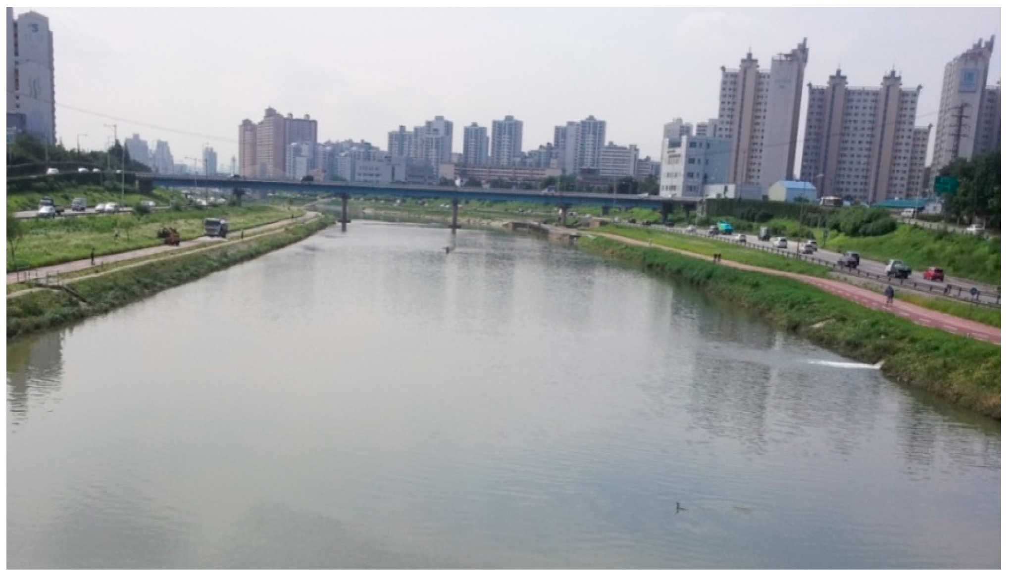
Anyangcheon stream is a tributary of the Han River (
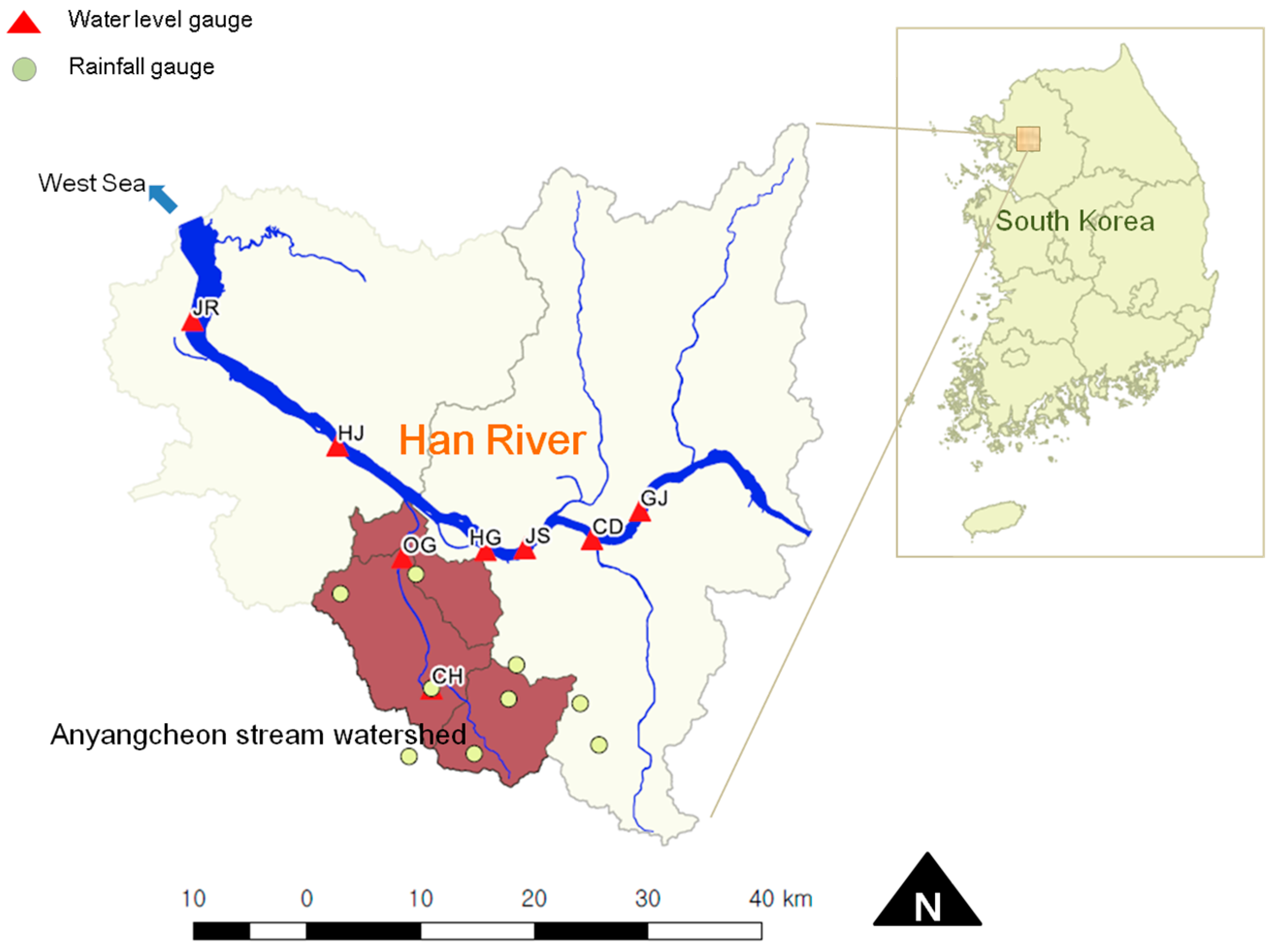
Figure 1). Located at the southwest part of the Seoul metropolitan area, the study area is the Anyangcheon stream watershed (
Figure 2), having an area of 286 km
2 and a main channel length of 32.5 km. Because many residential (urbanized) districts are situated in the upstream (downstream) area, reliable flood warning is crucial to mitigate damage in this area. Ogeumgyo Bridge, the flood prediction site located 6 km upstream of the junction of the Han River, is significantly affected by the backwater effect from the river. Flood flow in the Han River is largely influenced by the release from Paldang reservoir and the tidal effect from sea water at the end of the river. Moreover, a series of tributaries such as Wangsukcheon, Tancheon, Jungnangcheon, and Anyangcheon streams flow to the Han River.
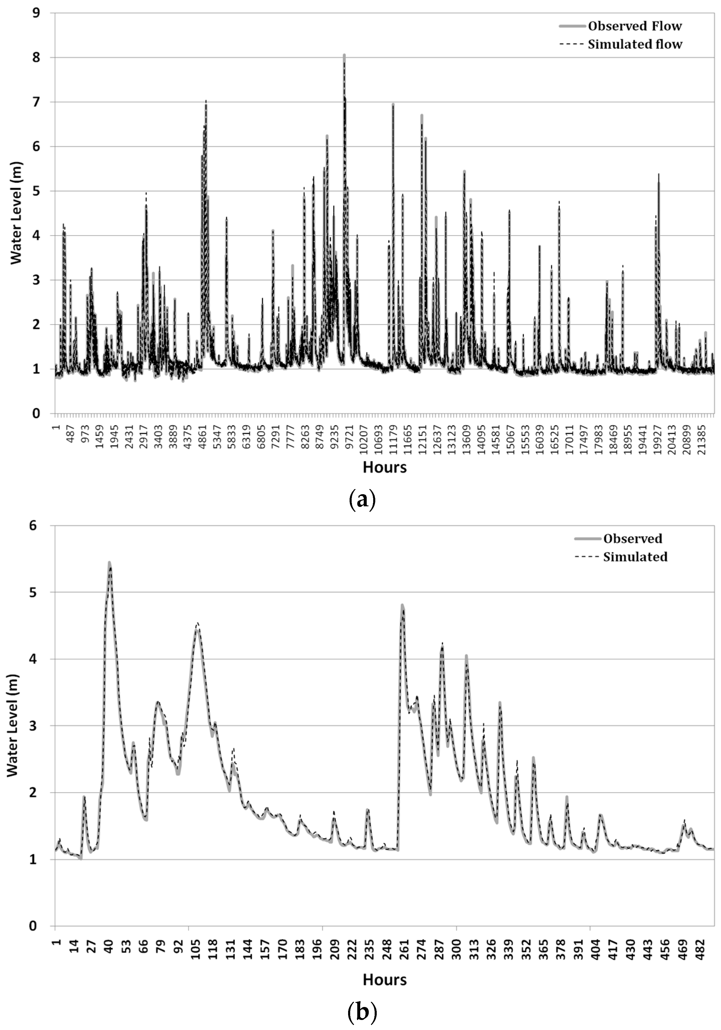
In this study, to predict flood water levels at the Ogeumgyo Bridge, hourly rainfall and water level data were used. Water level data from four gauging stations at the Han River were used to consider the backwater effect from the river, which is affected by release from Paldang reservoir and tidal conditions. To compute average rainfall, a Thiessen polygon was constructed including nine rainfall gauging stations. Data used for this study include hourly water level series from six gauging stations of Ogeumgyo (OG), Chunghungyo (CH), Jeonryu (JR), Haengjudaegyo (HJ), Hangangdaegyo (HG), and Jamsugyo (JS) and basin-averaged hourly rainfall series obtained from the Water Management Information System (WAMIS) provided by the Ministry of Land, Infrastructure and Transport (MOLIT), South Korea. The locations of the gauging stations are shown in
Figure 2 and
Figure 3. This study focused on water level forecasts during the rainy season. Only data recorded during the monsoon period from 21 June to 20 September for 2007–2016 were used in this study because this period is considered as the main rainy season in South Korea. These data collected were divided into two subsets. Data from the first six years were used for training, whereas those from the remaining four years were used for testing the model.
2.2. Artificial Neural Network Model
The human brain is made up of huge networks of complex neurons connected by a substance called synapse and is able to define its own rules based on experience. Inspired by the structure of the human brain, McCulloch and Pitts first proposed an ANN [
29], and various ANN models have since been developed. An ANN model is a data-driven mathematical model having the ability to solve problems by learning neurons without inputting direct knowledge or physical processes. The ANN model is capable of identifying complex nonlinear relationships between inputs and outputs without needing to understand the nature of the phenomenon [
30].
The most widely used neural network is the multilayer perceptron [
30] (
Figure 4), in which neurons are organized in input, hidden, and output layers interconnected by their own connection strengths. The network is optimized through training. Computation of the ANN outputs the weighted sum of external stimuli entering the input layer through the activation function. ANN is considered to be a fairly simple and cost-effective tool for obtaining solutions through the procedures of defining distributions, training, and validation.
The three-layered feed forward neural network which has been widely used in hydrologic forecasting models can be represented by a linear combination of the transformed input variables as:
where
is the forecasted
th output value,
is the activation function for the output neuron,
is the number of output neurons,
is the weight connecting the
th neuron in the hidden layer and
th neuron in the output layer,
is the activation function for the hidden neuron,
is the number of hidden neurons,
is the weight connecting the
th neuron in the input layer and
th neuron in the hidden layer,
is the
th input variable,
is the bias for the
th hidden neuron, and
is the bias for the th
th output neuron [
31]. Neural networks can learn their weights and biases through a training process. In the present study, ANN weights and biases were updated by a back-propagation algorithm which was developed originally by Rumelhart et al. (1986) [
32]. The algorithm is based on the gradient descent method with the objective of minimizing the sum of errors of the network in Equation (2).
where
is the error for all input patterns,
is the error based on the squared difference between target outputs
and forecasted outputs
for pattern p [
33].
2.3. ANN Model Development
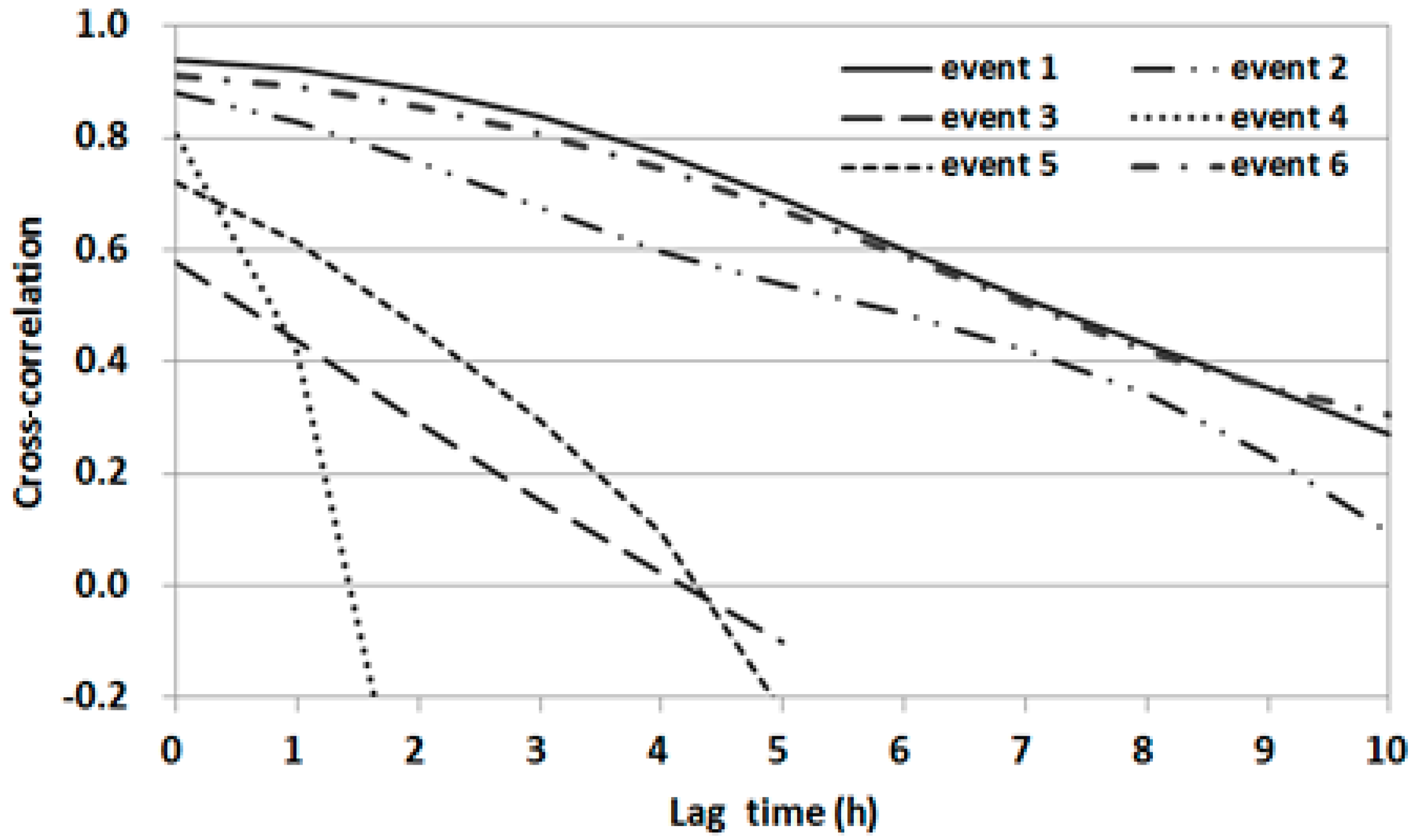
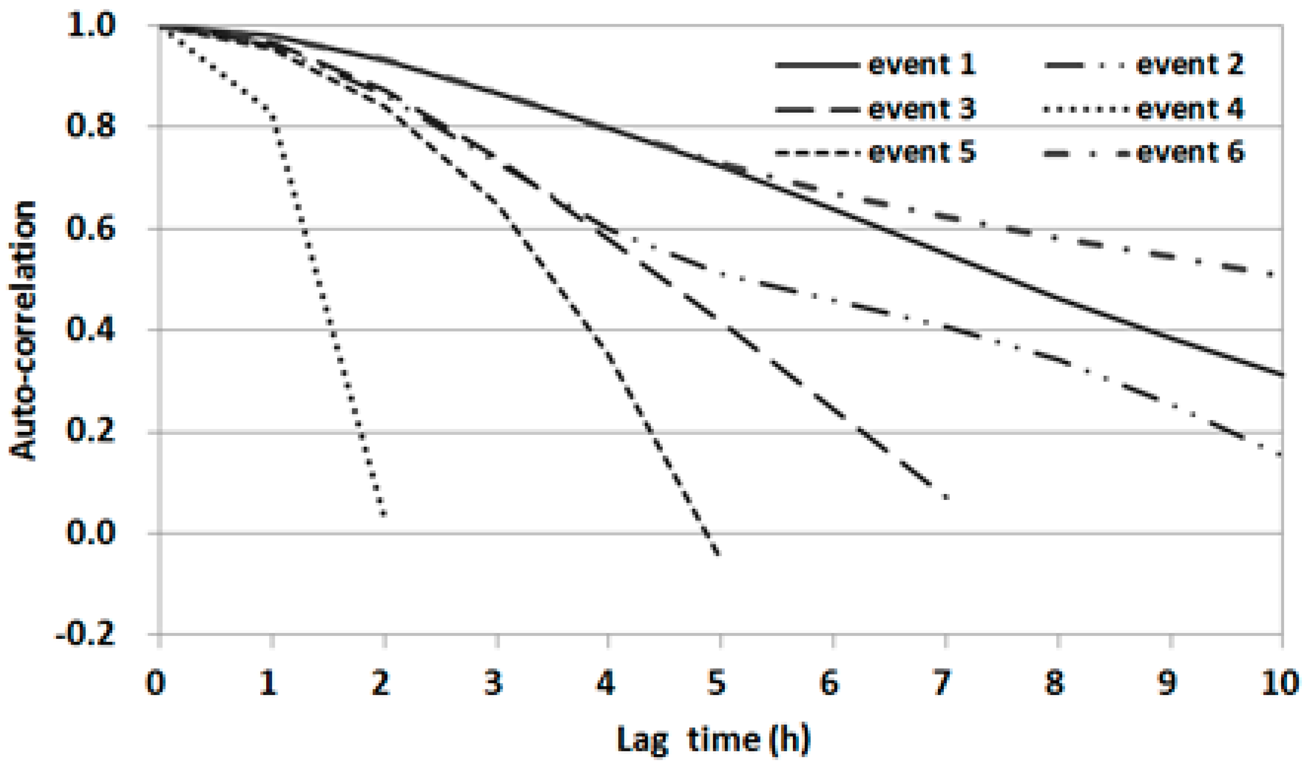
In this study, three types of ANN models were built to forecast water levels with 1, 2, and 3 h lead-times, respectively. The two most important steps in the ANN model development are the selection of significant input variables and the optimization of network architecture. Usually, significant input variables of networks can be determined through statistical analysis of data series such as the cross-correlation function (CCF), auto-correlation function (ACF), and partial auto-correlation function (PACF), as suggested by Sudheer and Jain [
34]. In this study, correlation analyses were performed for total period data, and
Figure 5,
Figure 6,
Figure 7 and
Figure 8 illustrated the results for six events given in
Table 1.
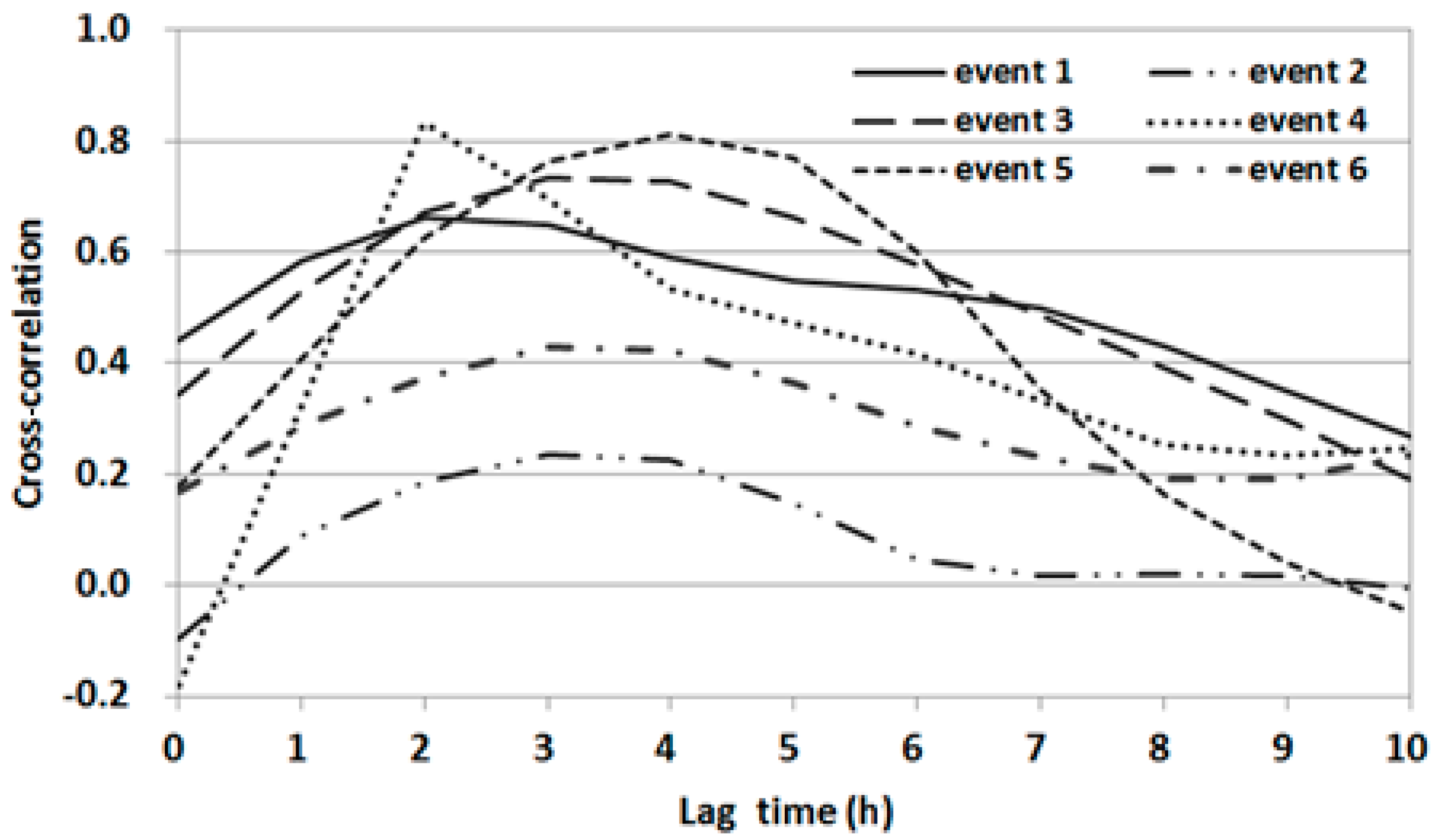
The CCFs between the water level series at output station OG and the areal rainfall series for six flood events are shown in
Figure 5. The magnitudes of CCF values varied considerably with the lag time for each event. Events 1 and 4 showed a high correlation with 2 h of lag time in the water level data on averaged rainfall data at any time. However, event 5 showed significant correlation with 3 to 5 h of lag time. A specific dominant cross-correlation process could not be determined. Furthermore, very low CCFs were found for events 2 and 6 even though the events showed high peaks. This might be attributed to an effect of the boundary conditions of the water level at the confluence of the tributary of interest and the main river.
The CCFs between the water level at OG and the upstream water level at CH were estimated for each event, as shown in
Figure 6. The CCF for event 1 showed a significant correlation with a lag time of up to 7 h, whereas those for events 3, 5, and 6 showed significant correlation with lag times of up to 4 h. For event 4, which had short flood duration, the CCF rapidly declined after a lag time of 2 h. The low CCF for event 2 indicated that the water level could be affected by other factors such as downstream hydrologic conditions.
The CCF between the water level at OG and that at HJ located on the main river is shown in
Figure 7. A highly significant correlation was found for events 1, 2, and 6. The CCFs decreased gradually with an increase in lag time, which indicates that the output water level data at OG are strongly correlated with the water level data on the main river. The same processes were applied to estimate the CCFs between the output and input variables of water levels at JR, HG, and JS, which also showed various correlations for each event.
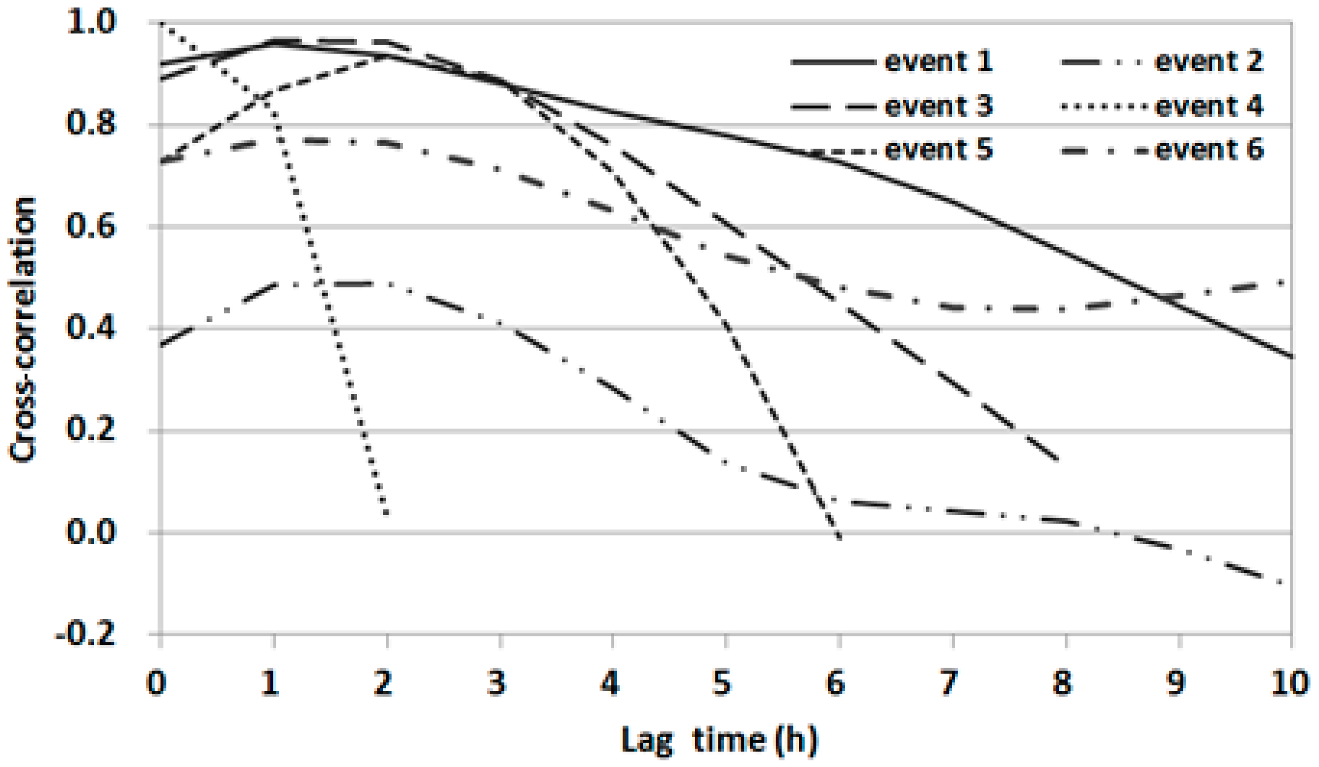
The ACFs from 0 to 10 h lag times were estimated for the water level data at OG. A significant correlation up to about 8 h of lag time was found for events 1 and 6 (
Figure 8). However, the ACF for event 4 decreased sharply after 1 h of lag time. As shown in
Figure 8, the ACFs differed significantly among events and decreased gradually or rapidly with an increase in lag time.
On the basis of the statistical analysis of correlation presented above, the input and output data nonlinearly correlated with each other. This nonlinearity means that the backwater effect is inherent in the output data. In the case that backwater effect is apparent in target water level data, the ANN model will be useful to deal with nonlinear features. Weak cross-correlations for some events indicated that it might be difficult to determine the specific dominant lag time of input variables in advance in the case of our study area where backwater effect from the main river exists. Therefore, a trial and error procedure was used in this study to identify the optimal input vector using various lag times of input variables.
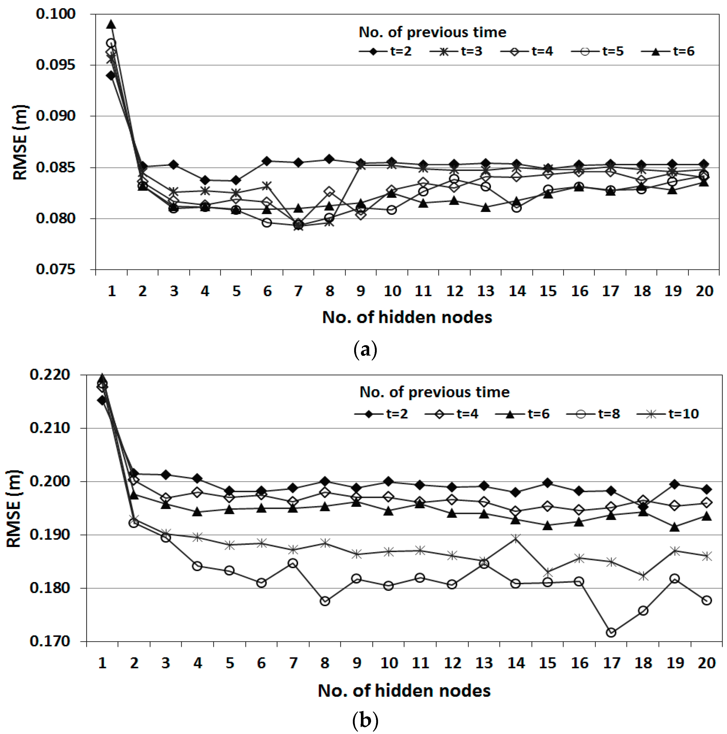
The optimal structure was determined by considering input variables from the current time (t) to previous hours (from t-1 to t-10). Statistical errors of the training set were calculated for the different number of nodes in the hidden layer. Liang and Sun [
35] proposed that number of hidden neurons should be half size of the input nodes plus output nodes for better forecasting accuracy. According to this guide, the numbers of hidden nodes within 39 were tested considering the size of input nodes for the most complex ANN structure treated in the present study. The number of hidden nodes was progressively increased from 1 to 39, and then the ANN model performance was evaluated by the measure of root mean square error (RMSE). The results showed the minimum RMSE when the numbers of hidden nodes around 20 were used. Therefore, the optimal number of hidden nodes was determined to be between 1 and 20 in this study.
For each set of hidden nodes and input variables, the network was trained to minimize the root mean square error (RMSE) at one output layer by using a back-propagation algorithm. The learning rate was set to 0.01, and the hyperbolic tangent sigmoid function was used as the activation function for the hidden layer. The early stopping method has been widely used to avoid the over-fitting problem, in which, after dividing the data in three data sets, training, cross-validation, and testing, the output error of training and validation in each epoch is monitored and training is stopped when the cross-validation error is minimum [
25]. However, the technique was not applied in the present study due to a large number of training cases for more than two thousands networks. A maximum epoch of 5000 was adopted for training, which was determined from the preliminary performance tests for the complex ANN structures.
ANN models were first trained by using the training data set, 60% of the total data, to obtain an optimized set of connection weights. These models were then tested by using the remaining data, 40% of the total data. These models were then compared by using three statistical measures: goodness of fit of RMSE, determination coefficient (R
2), and Nash–Sutcliffe efficiency (NSE) given by
where
is the observed water level,
is the mean value,
is the forecasted water level from the model, and N is the number of data points.
