Reconstruction of an Acid Water Spill in a Mountain Reservoir

 and
and
Abstract
:1. Introduction
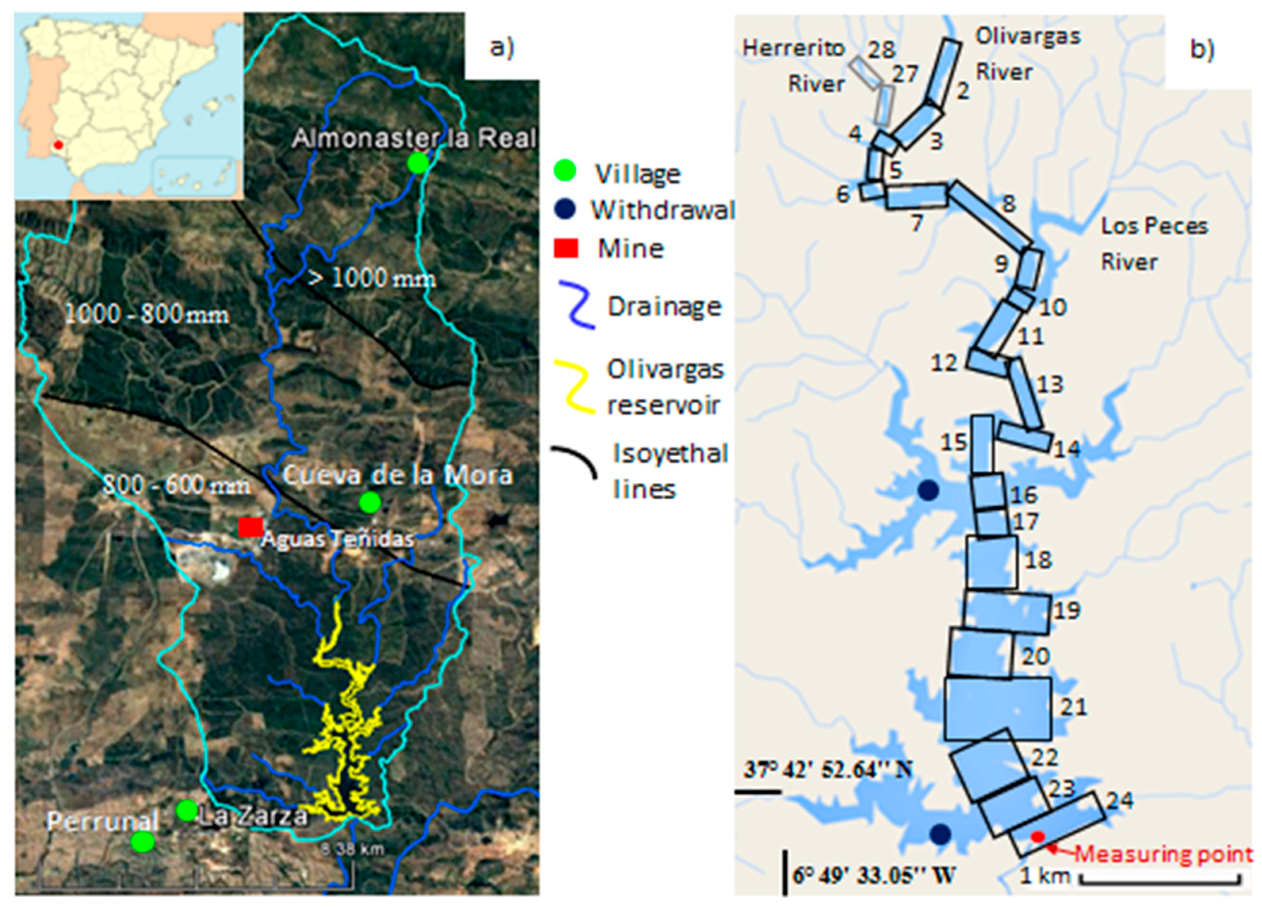
2. Study Site Description
3. Materials and Methods
3.1. On-Site Measurements
3.2. Model Description and Application
3.2.1. General Model Description
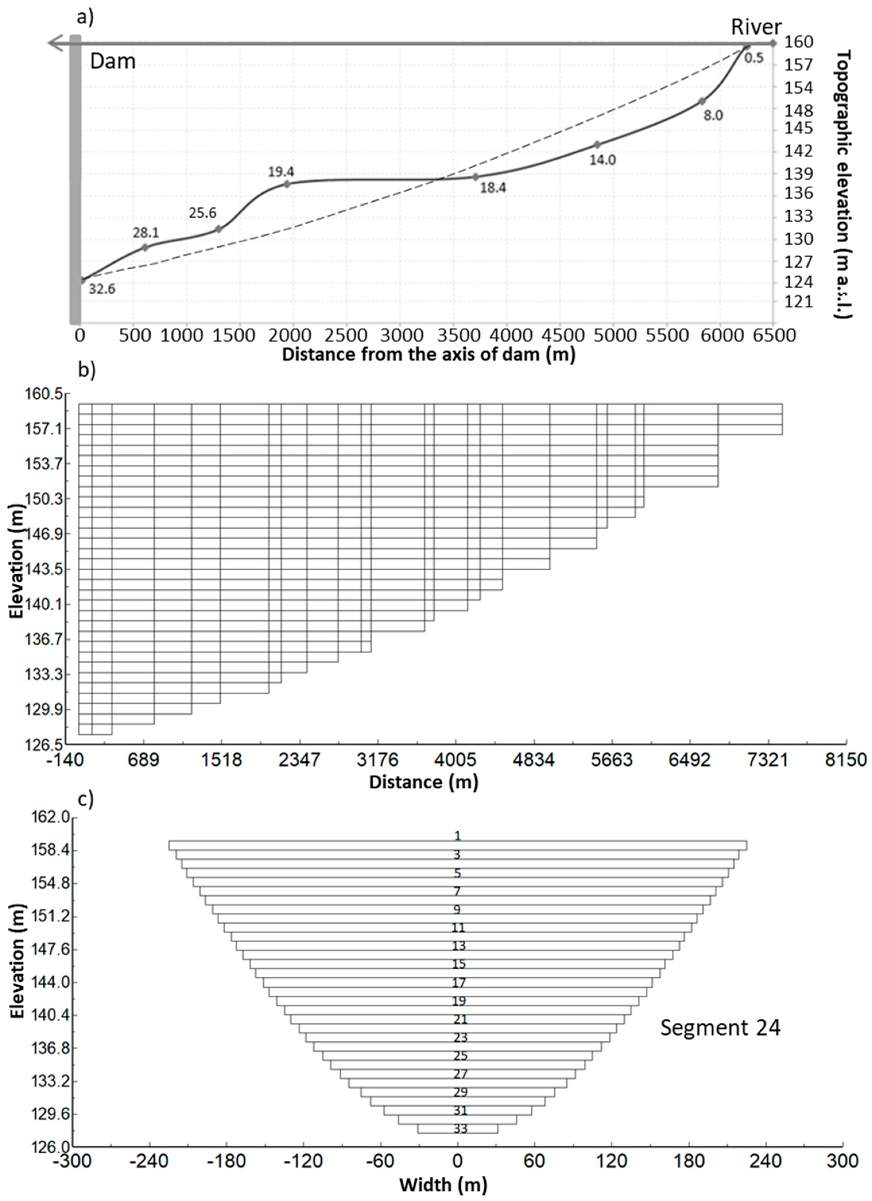
3.2.2. Geometry and Bathymetry Derivation
3.2.3. Data Sources
- -
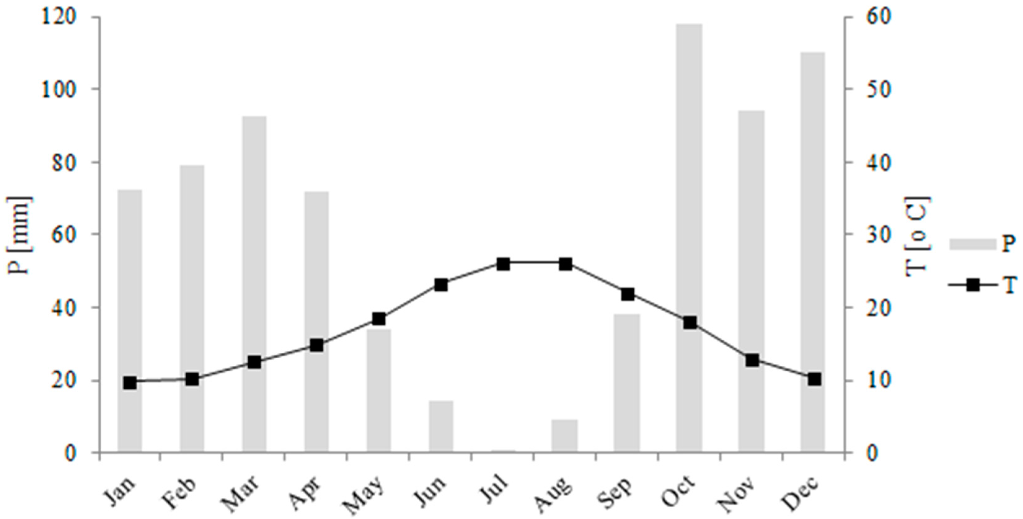
- Meteorological data: Air temperature, relative humidity, wind speed and direction, precipitation and solar radiation data were obtained from the Meteorological Spanish Survey [30] from El Campillo Station, located 19.25 km east of the Olivargas Reservoir. Dew point temperature was calculated from relative humidity and air temperature [31]. The precipitation temperature was obtained from the dew point. The percentage of cloud cover was calculated according to the methods of [32,33,34] from the solar radiation data, with Glover and McCulloch’s method providing the best result.
- -
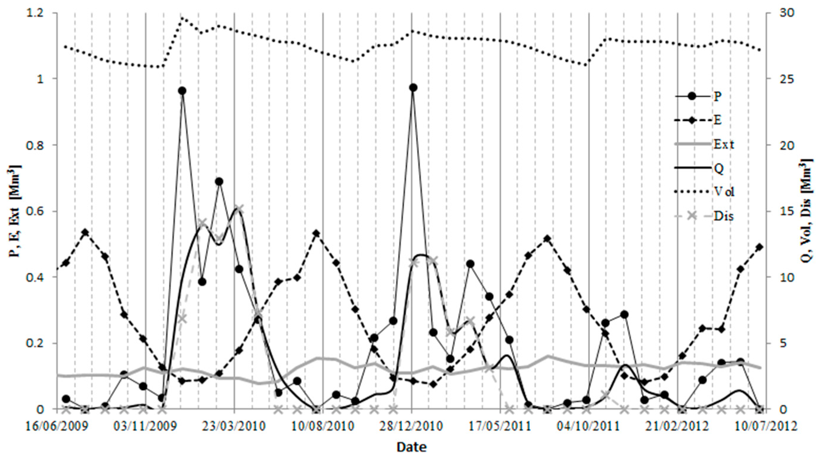
- Flow into the reservoir: The only inflow considered was from the Olivargas River, which, in the rainy season, contributes more than 90% of the incoming flow. The river flow database was generated with the SWAT code. A more detailed description of the SWAT model application to the region can be found in [28,35,36].
- -
- Inflow water quality:
- ○
- The water temperature of the inflow was obtained from continuous measurements by the CTD-DIVER installed in the Olivargas River.
- ○
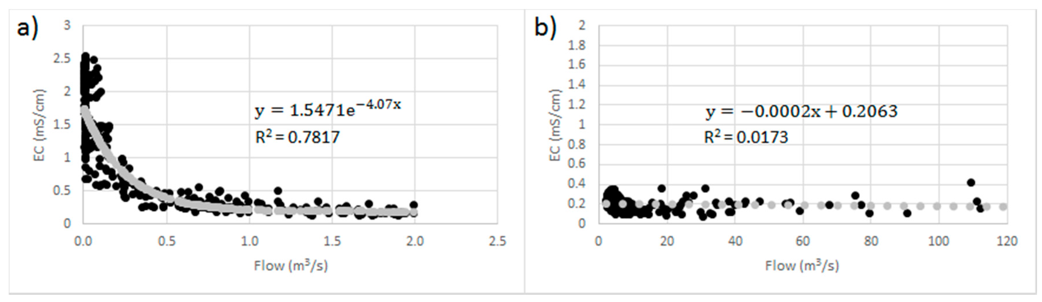
- The total dissolved solids (TDS) of the inflow was calculated from the EC measured continuously by a CTD-DIVER installed in the Olivargas River and the molecular weight of CaSO4 (the dominant salt in the reservoir).
- ○
- The DO of the inflow was calculated from the air-water equilibrium, water temperature and ionic strength.
- ○
- The labile dissolved organic matter (LDOM) and the alkalinity of the inflow were obtained from the average of four sampling campaigns and considered constant throughout the modeling period. Total inorganic carbon (TIC) was obtained from the measured values of pH and alkalinity.
- -
- Extractions: There are two water withdrawal points instrumented inside the reservoir: one for the mining company, MATSA, operating the Aguas Teñidas mine located near segment 16, and another owned by the drinking water company, GIAHSA, located near segment 23 (blue dots, Figure 1b).
- -
- Temperature, TDS, and DO profiles were taken at the measuring point near the dam (Figure 1b) on the 6 July 2009.
- -
- The LDOM profile was obtained at the measuring point on 30 January 2010.
- -
- The alkalinity profile was obtained on 4 September 2009, at the measuring point. The TIC profile was obtained from the alkalinity and pH values.
4. Results and Discussion
4.1. General Calibration of Model
4.2. Hydrodynamic Modeling
4.2.1. Water Head
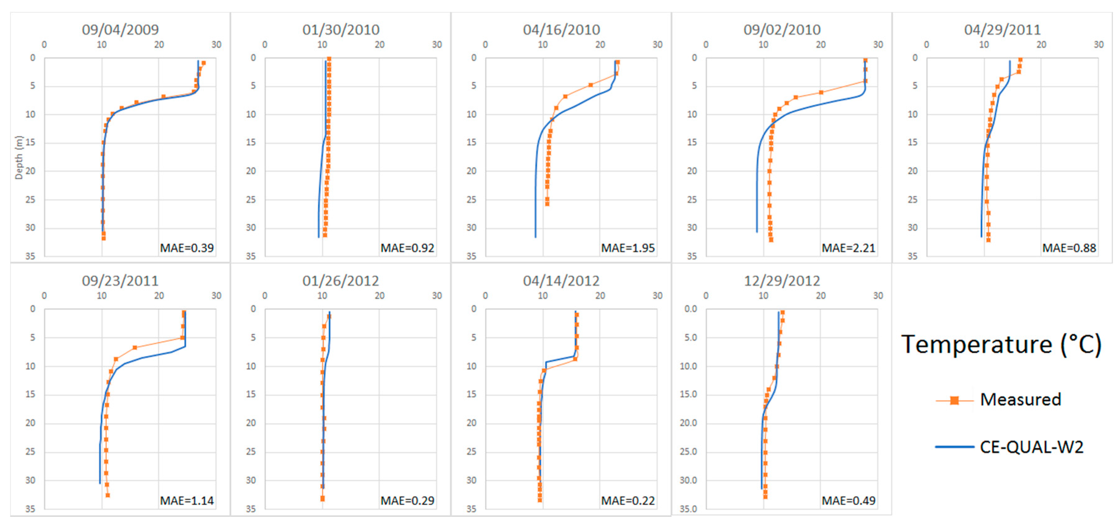
4.2.2. Temperature
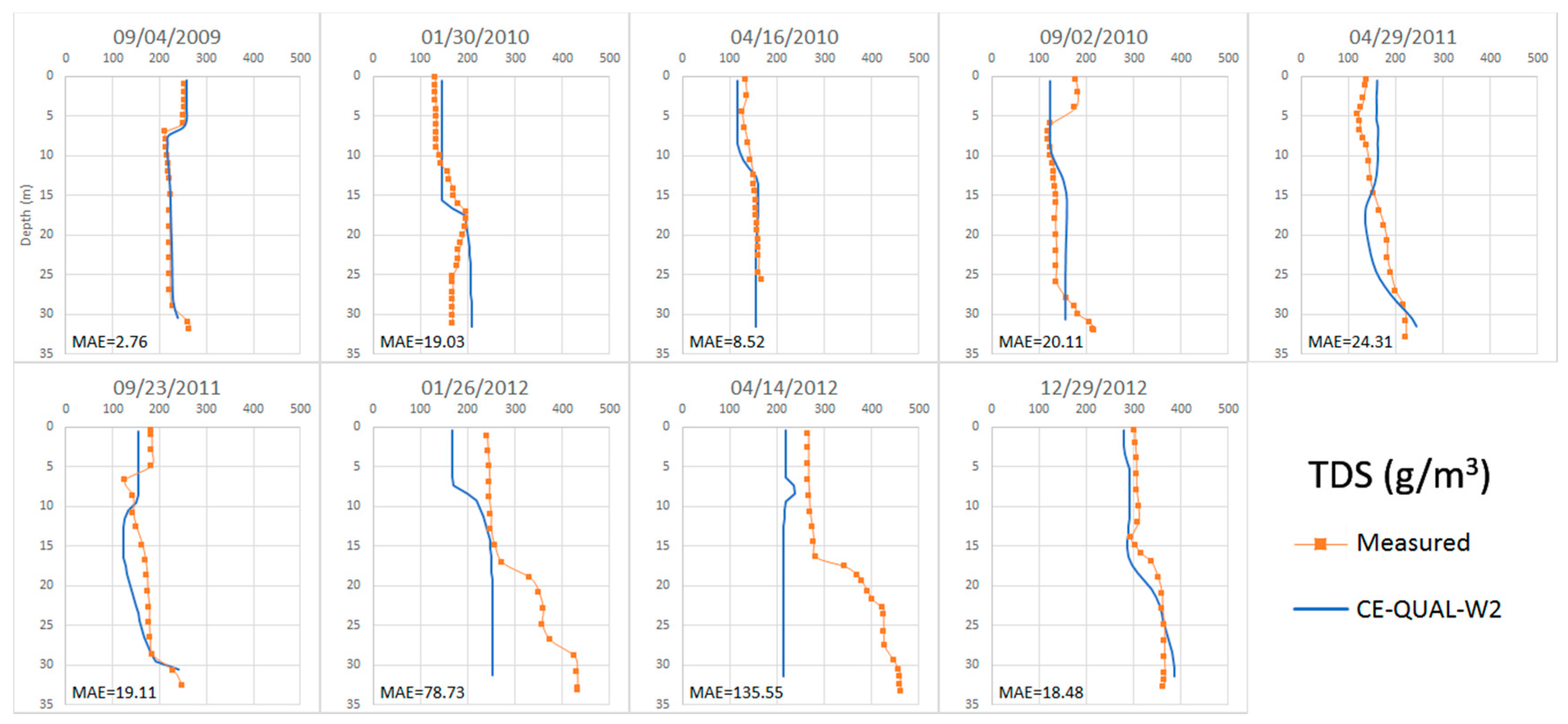
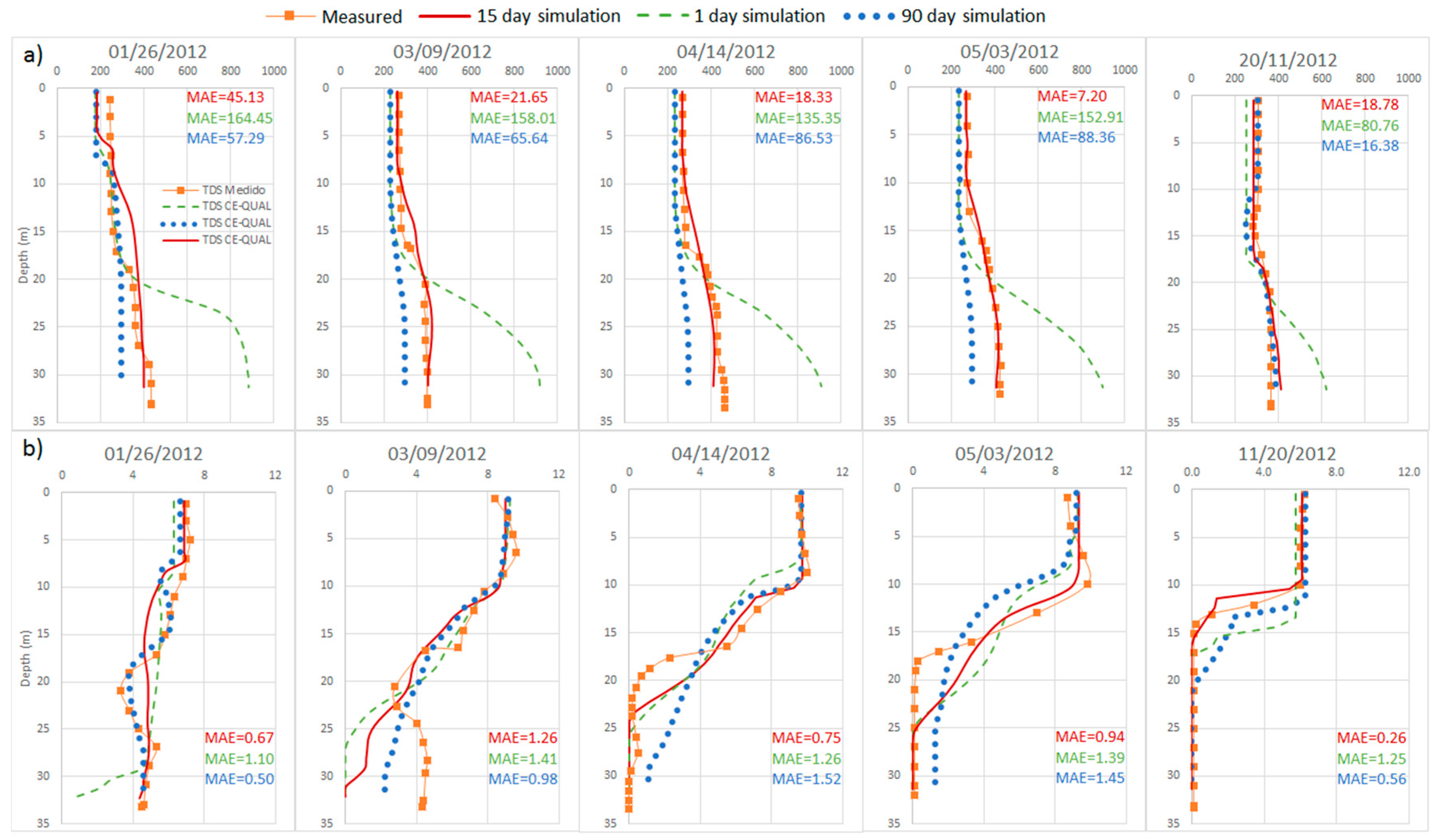
4.2.3. Total dissolved solids (TDS)
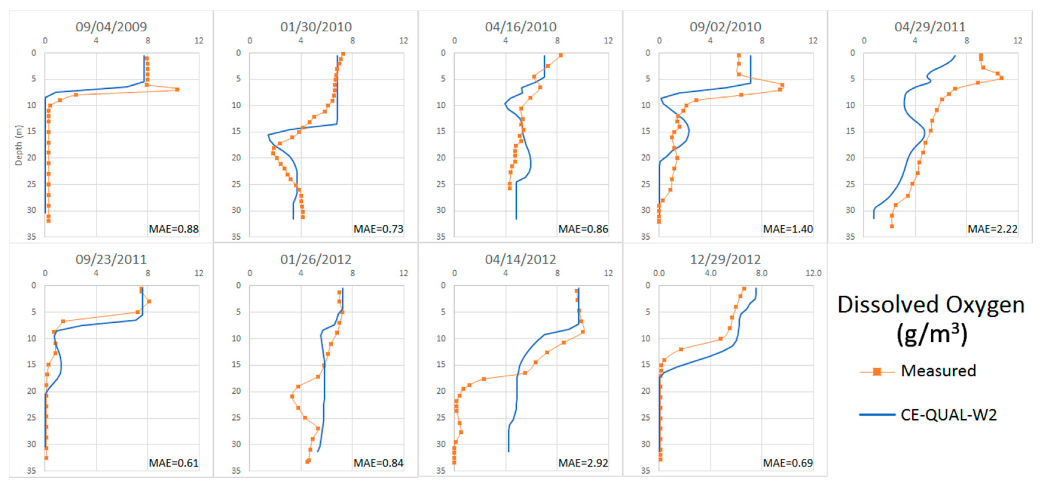
4.2.4. Dissolved Oxygen
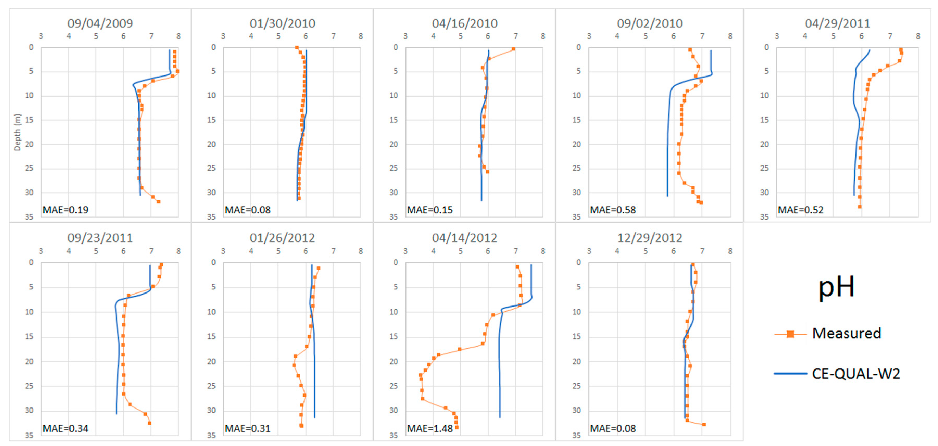
4.2.5. pH
4.3. Calibration of the Anomalous Period
5. Conclusions
Acknowledgments
Author Contributions
Conflicts of Interest
References
- Mooij, W.M.; Trolle, D.; Jeppesen, E.; Arhonditsis, G.; Belolipetsky, P.V.; Chitamwebwa, D.B.R.; Degermendzhy, A.G.; De Angelis, D.L.; De Senerpont Domis, L.N.; Downing, A.S.; et al. Challenges and opportunities for integrating lake ecosystem modeling approaches. Aquat. Ecol. 2010, 44, 633–667. [Google Scholar] [CrossRef] [Green Version]
- Cole, T.M.; Wells, S.A. Hydrodynamic Modeling with Application to CE-QUAL-W2. En Workshop Notes; Portland State University: Portland, OR, USA, 2000. [Google Scholar]
- Cole, T.M.; Wells, S.A. CE-QUAL-W2: A Two-Dimensional, Laterally Averaged, Hydrodynamic and Water Quality Model; Version 4.0; Portland State Univeristy: Portland, OR, USA, 2015; Available online: http://archives.pdx.edu/ds/psu/12049 (accessed on 14 February 2015).
- Zouabi-Aloui, B.; Adelana, S.M.; Gueddari, M. Effects of selective withdrawal on hydrodynamics and water quality of a thermally stratified reservoir in the southern side of the Mediterranean Sea: A simulation approach. Environ. Monit. Assess. 2015, 187, 1–19. [Google Scholar] [CrossRef] [PubMed]
- Fataei, E.; Moghadam, D.A.; Nasehi, F. Prediction of thermal stratification of Seymareh Dam using CE-QUAL-W2. Model. Adv. Bot. Res. 2014, 5, 150–159. [Google Scholar] [CrossRef]
- Wells, S.A.; Wells, V.I.; Berger, C. Impact of Phosphorus Loading from the Watershed on Water Quality Dynamics in Lake Tenkiller, Oklahoma, USA; World Environmental and Water Resources Congress: Sacramento, CA, USA, 2012; pp. 888–899. [Google Scholar] [CrossRef]
- White, J.D.; Prochnow, S.J.; Filstrup, C.T.; Scott, J.T.; Byars, B.W.; Zygo-Flynn, L. A combined watershed-water quality modeling analysis of the Lake Wako reservoir: I. Calibration and confirmation of predicted water quality. Lake Reserv. Manag. 2010, 26, 147–158. [Google Scholar] [CrossRef]
- Wu, T.; Luo, L.; Qin, B.; Cui, G.; Yu, Z.; Yao, Z. A vertically integrated eutrophication model and its application to a river-style reservoir—Fuchunjiang, China. J. Environ. Sci. 2009, 21, 319–327. [Google Scholar] [CrossRef]
- Khangaonkar, T.; Yang, Z. Dynamic response of stream temperatures to boundary and inflow perturbation due to reservoir operations. River Res. Appl. 2008, 24, 420–433. [Google Scholar] [CrossRef]
- Ma, S.; Kassinos, S.C.; Kassinos, D.F.; Akylas, E. Effects of selective water withdrawal schemes on thermal stratification in Kouris Dam in Cyprus. Lake Reserv. Manag. 2008, 13, 51–61. [Google Scholar] [CrossRef]
- Afshar, A.; Masoumi, F. Waste load reallocation in river–reservoir systems: Simulation–optimization approach. Environ. Earth Sci. 2016, 75, 1–14. [Google Scholar] [CrossRef]
- Jeznach, L.C.; Jones, C.; Matthews, T.; Tobiason, J.E.; Ahlfeld, D.P. A framework for modeling contaminant impacts on reservoir water quality. J. Hydrol. 2016, 537, 322–333. [Google Scholar] [CrossRef]
- Torres, E.; Galván, L.; Ruiz Cánovas, C.; Soria-Píriz, S.; Arbat-Bofill, M.; Nardi, A.; Papaspyrou, S.; Ayora, C. Oxycline formation induced by Fe(II) oxidation in a water reservoir affected by Acid Mine Drainage modeled using a 2D hydrodynamic and water quality model—CE-QUAL-W2. Sci. Total Environ. 2016, 562, 1–12. [Google Scholar] [CrossRef] [PubMed]
- Narasimhan, B.; Srinivasan, R.; Bednarz, S.T.; Ernst, M.R.; Allen, P.M. A comprehensive modeling approach for reservoir water quality assessment and management due to point and nonpoint source pollution. Trans. ASABE 2010, 53, 1605–1617. [Google Scholar] [CrossRef]
- Yu, S.J.; Lee, J.Y.; Ryong, H.S. Effect of a seasonal diffuse pollution migration on natural organic matter behavior in a stratified dam reservoir. J. Environ. Sci. 2010, 22, 908–914. [Google Scholar] [CrossRef]
- Noori, R.; Yeh, H.D.; Ashrafi, K.; Rezazadeh, N.; Bateni, S.M.; Karbassi, A.; Kachoosangi, F.T.; Moazami, S. A reduced-order based CE-QUAL-W2 model for simulation of nitrate concentration in dam reservoirs. J. Hydrol. 2015, 530, 645–656. [Google Scholar] [CrossRef]
- Park, Y.; Cho, K.H.; Kang, J.H.; Lee, S.W.; Kim, J.H. Developing a flow strategy to reduce nutrient load in a reclaimed multi-reservoir system using a 2D hydrodynamic and water quality model. Sci. Total Environ. 2014, 466, 871–880. [Google Scholar] [CrossRef] [PubMed]
- Berger, C.J.; Wells, S.A. Modeling the effects of macrophytes on hydrodynamics. J. Environ. Eng. 2008, 134, 778–788. [Google Scholar] [CrossRef]
- Kuo, J.T.; Lung, W.S.; Yang, C.P.; Liu, W.C.; Yang, M.D.; Tang, T.S. Eutrophication modeling of reservoirs in Taiwan. Environ. Model. Softw. 2006, 21, 829–844. [Google Scholar] [CrossRef]
- Buccola, N.L.; Risley, J.C.; Rounds, S.A. Simulating future water temperatures in the North Santiam River, Oregon. J. Hydrol. 2016, 535, 318–330. [Google Scholar] [CrossRef]
- Molina-Navarro, E.; Trolle, D.; Martínez-Pérez, S.; Sastre-Merlín, A.; Jeppesen, E. Hydrological and water quality impact assessment of a Mediterranean limno-reservoir under climate change and land use management scenarios. J. Hydrol. 2014, 509, 354–356. [Google Scholar] [CrossRef]
- Lee, C.; Foster, G. Assessing the potential of reservoir outflow management to reduce sedimentation using continuous turbidity monitoring and reservoir modelling. Hydrol. Process. 2013, 27, 1426–1439. [Google Scholar] [CrossRef]
- Samal, N.R.; Matonse, A.H.; Mukundan, R.; Zion, M.S.; Pierson, D.C.; Gelda, R.K.; Schneiderman, E.M. Modelling potential effects of climate change on winter turbidity loading in the Ashokan Reservoir, NY. Hydrol. Process. 2013, 27, 3061–3074. [Google Scholar] [CrossRef]
- Choi, J.H.; Jeong, S.A.; Park, S.S. Longitudinal-vertical hydrodynamic and turbidity simulations for prediction of dam reconstruction effects in Asian monsoon area. J. Am. Water Resour. Assoc. 2007, 43, 1444–1454. [Google Scholar] [CrossRef]
- Bowen, J.D.; Hieronymus, J.W. A CE-QUAL-W2 model of Neuse Estuary for total maximum daily load development. J. Water Resour. Plann. Manag. 2003, 129, 283–294. [Google Scholar] [CrossRef]
- Debele, B.; Srinivasan, R.; Parlange, J.Y. Coupling upland watershead and downstream waterbody hydrodynamic and water quality models (SWAT and DE-CUAL-W2) for better water resources management in complex river basins. Environ. Model. Assess. 2008, 13, 135–153. [Google Scholar] [CrossRef]
- Cánovas, C.R.; Olías, M.; Macias, F.; Torres, E.; San Miguel, E.G.; Galván, L.; Ayora, C.; Nieto, J.M. Water acidification trends in a reservoir of the Iberian Pyrite Belt (SW Spain). Sci. Total Environ. 2016, 541, 400–411. [Google Scholar] [CrossRef] [PubMed]
- Galván, L.; Olías, M.; Cánovas, C.R.; Sarmiento, A.M.; Nieto, J.M. Hydrological modeling of a watershed affected by acid mine drainage (Odiel River, SW Spain). Assessment of the pollutant contributing areas. J. Hydrol. 2016, 540, 196–206. [Google Scholar] [CrossRef]
- Tornos, F. Environment of formation and styles of volcanogenic massive sulfides: The Iberian Pyrite Belt. Ore Geol. Rev. 2006, 28, 259–307. [Google Scholar] [CrossRef]
- Agencia Estatal de Meteorología, AEMET. Spain. Available online: http://www.aemet.es (accessed on 22 May 2015).
- Hess, S.L. Introduction to Theoretical Meteorology, 1st ed.; Holt, Rinehart, and Winston: New York, NY, USA, 1978; p. 362. ISBN 0882758578. [Google Scholar]
- Prescott, J. Evaporation from a water surface in relation to solar radiation. Q. J. R. Meteorol. Soc. 1940, 64, 114–118. [Google Scholar]
- Glover, J.; McCulloch, J.S.G. The empirical relation between solar radiation and hours of sunshine. Q. J. R. Meteorol. Soc. 1958, 84, 172–175. [Google Scholar] [CrossRef]
- Black, J.N. The distribution of solar radiation over the earth’s surface. Arch. Meteorol. Geophys. Bioklimatol. Ser. B 1956, 7, 165–189. [Google Scholar] [CrossRef]
- Galván, L.; Olías, M.; Fernandez de Villarán, R.; Domingo Santos, J.M.; Nieto, J.M.; Sarmiento, A.M.; Cánovas, C.R. Application of the SWAT model to an AMD-affected river (Meca River, SW Spain). Estimation of transported pollutant load. J. Hydrol. 2009, 377, 445–454. [Google Scholar] [CrossRef]
- Galván, L.; Olías, M.; Izquierdo, T.; Cerón, J.C.; Fernández de Villarán, R. Rainfall estimation in SWAT: An alternative method to simulate orographic precipitation. J. Hydrol. 2014, 509, 257–265. [Google Scholar] [CrossRef]
- Caissie, D.; El-Jabi, N.; Satish, M.G. Modelling of maximum daily water temperatures in a small stream using air temperatures. J. Hydrol. 2001, 251, 14–28. [Google Scholar] [CrossRef]
- Willmott, C.J.; Matsuura, K. Advantages of the mean absolute error (MAE) over the root mean square error (RMSE) in assessing average model performance. Clim. Res. 2005, 30, 79–82. [Google Scholar] [CrossRef]
- Cánovas, C.R.; Olías, M.; Nieto, J.M.; Galván, L. Wash-out processes of evaporitic sulfate salts in the Tintoriver: Hydrogeochemical evolution and environmental impact. Appl. Geochem. 2010, 25, 288–301. [Google Scholar] [CrossRef]
- Stumm, W.; Morgan, J.J. Aquatic Chemistry, Chemical Equilibra and Rates in Natural Waters, 3rd ed.; Wiley: New York, NY, USA, 1996; p. 1022. ISBN 0-471-51184-6. [Google Scholar]
- Sarmiento, A.M.; Olías, M.; Nieto, J.M.; Cánovas, C.R. Hydrochemical characteristics and seasonal influence on the pollution by acid mine drainage in the Odiel river Basin (SW Spain). Appl. Geochem. 2009, 24, 697–714. [Google Scholar] [CrossRef]
- Sanchez España, J.; Lopez Pamo, E.; Santofimia, E.; Aduvire, O.; Reyes, J.; Barettino, D. Acid mine drainage in the Iberian Pyrite Belt (Odiel river watershed, Huelva, SW Spain): Geochemistry, mineralogy and environmental implications. Appl. Geochem. 2005, 20, 1320–1356. [Google Scholar] [CrossRef]


| Variable | Value |
|---|---|
| Dam crest height *, m a.s.l. | 163 |
| Volume *, Mm3 | 28.5 |
| Total area *, km2 | 2.44 |
| Maximum depth *, m | 33 |
| Length *, km | 7.57 |
| Greatest width *, km | 1.6 |
| Spillway height, m a.s.l. | 158.7 |
| Number of withdrawal structures | 2 |
| Average percent for mining extraction, % | 45 |
| Average percent of extraction for domestic supply, % | 55 |
| Year of filling | 1983 |
| Coefficient | Olivargas Reservoir | Cole and Wells (2015) |
|---|---|---|
| Horizontal eddy viscosity, m2/s | 1.0 | 1.0 |
| Horizontal eddy diffusivity, m2/s | 1.0 | 1.0 |
| Interfacial friction factor, adim | 0.015 | 0.015 |
| Manning coefficient, s/m1/3 | 0.027 | - |
| Wind roughness height, m | 0.001 | 0.001 |
| Wind sheltering, adim | 1.2 | 0.1–0.9 |
| Fraction of heat lost to sediments added back to water column, adim | 1.0 | 1.0 |
| Fraction of solar radiation absorbed at the water surface, adim | 0.45 | 0.45 |
| Coefficient of bottom heat exchange, W/m2/s | 0.3 | 0.3 |
| Light extinction coefficient for pure water, m−1 | 0.45 | 0.25 or 0.45 |
| Extinction coefficient for inorganic solid, m−1 | 0.1 | 0.1 |
| Extinction coefficient for organic solid, m−1 | 0.1 | 0.1 |
| LDOM decay rate, day−1 | 0.1 | 0.1 |
| Sediment oxygen demand, g/m2/day | 0.2 | 0.1–0.5 |
© 2017 by the authors. Licensee MDPI, Basel, Switzerland. This article is an open access article distributed under the terms and conditions of the Creative Commons Attribution (CC BY) license (http://creativecommons.org/licenses/by/4.0/).
Share and Cite
Jofre-Meléndez, R.; Torres, E.; Ramos-Arroyo, Y.R.; Galván, L.; Ruiz-Cánovas, C.; Ayora, C. Reconstruction of an Acid Water Spill in a Mountain Reservoir. Water 2017, 9, 613. https://doi.org/10.3390/w9090613
Jofre-Meléndez R, Torres E, Ramos-Arroyo YR, Galván L, Ruiz-Cánovas C, Ayora C. Reconstruction of an Acid Water Spill in a Mountain Reservoir. Water. 2017; 9(9):613. https://doi.org/10.3390/w9090613
Chicago/Turabian StyleJofre-Meléndez, Rodolfo, Ester Torres, Yann René Ramos-Arroyo, Laura Galván, Carlos Ruiz-Cánovas, and Carlos Ayora. 2017. "Reconstruction of an Acid Water Spill in a Mountain Reservoir" Water 9, no. 9: 613. https://doi.org/10.3390/w9090613
APA StyleJofre-Meléndez, R., Torres, E., Ramos-Arroyo, Y. R., Galván, L., Ruiz-Cánovas, C., & Ayora, C. (2017). Reconstruction of an Acid Water Spill in a Mountain Reservoir. Water, 9(9), 613. https://doi.org/10.3390/w9090613