Measuring Recovery to Build up Metrics of Flood Resilience Based on Pollutant Discharge Data: A Case Study in East China
Abstract
1. Introduction
2. Methods
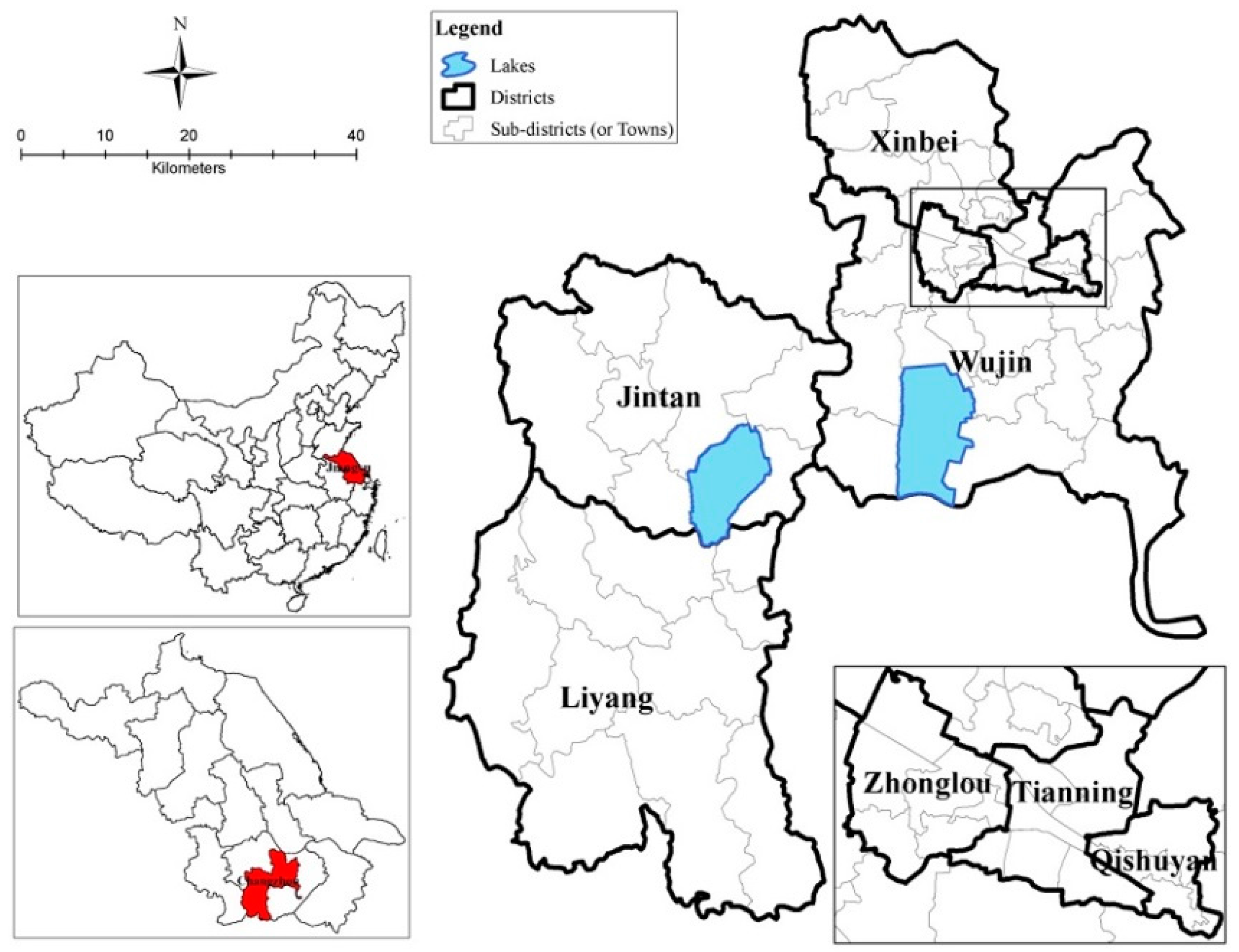
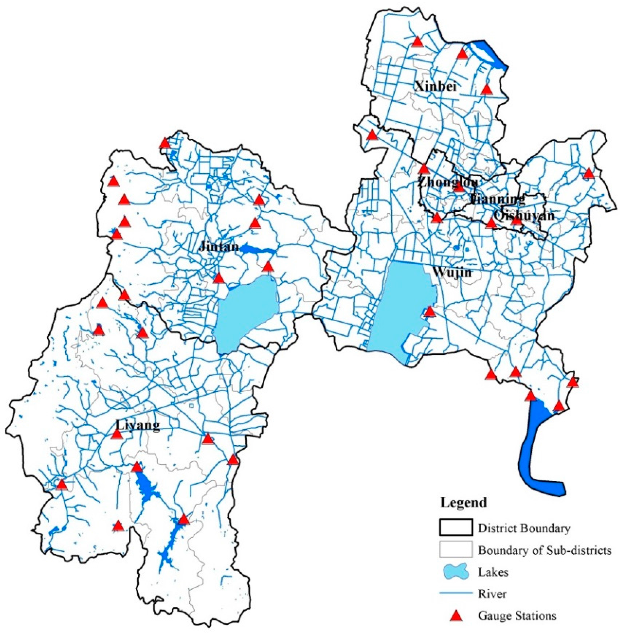
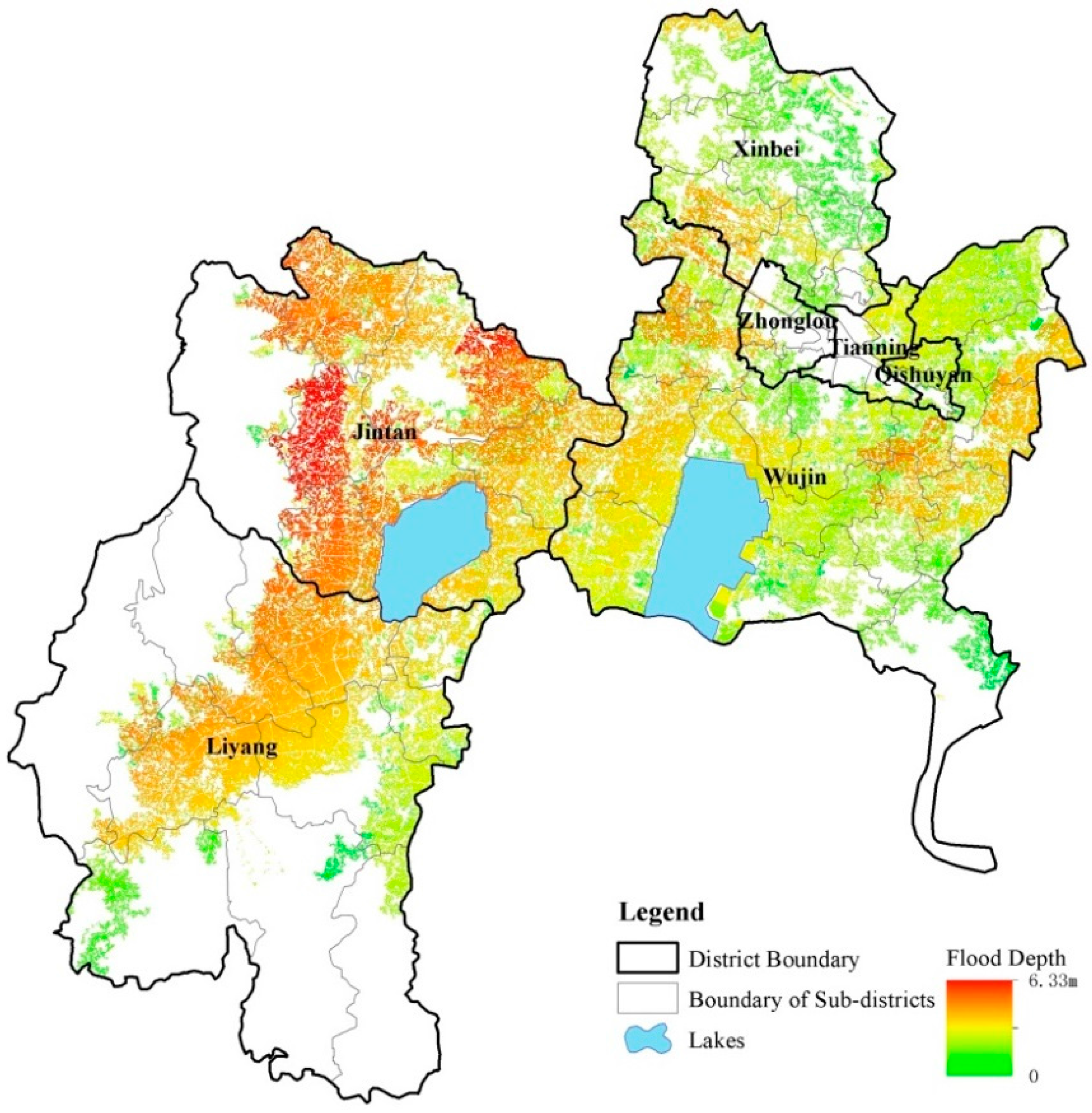
2.1. Study Area
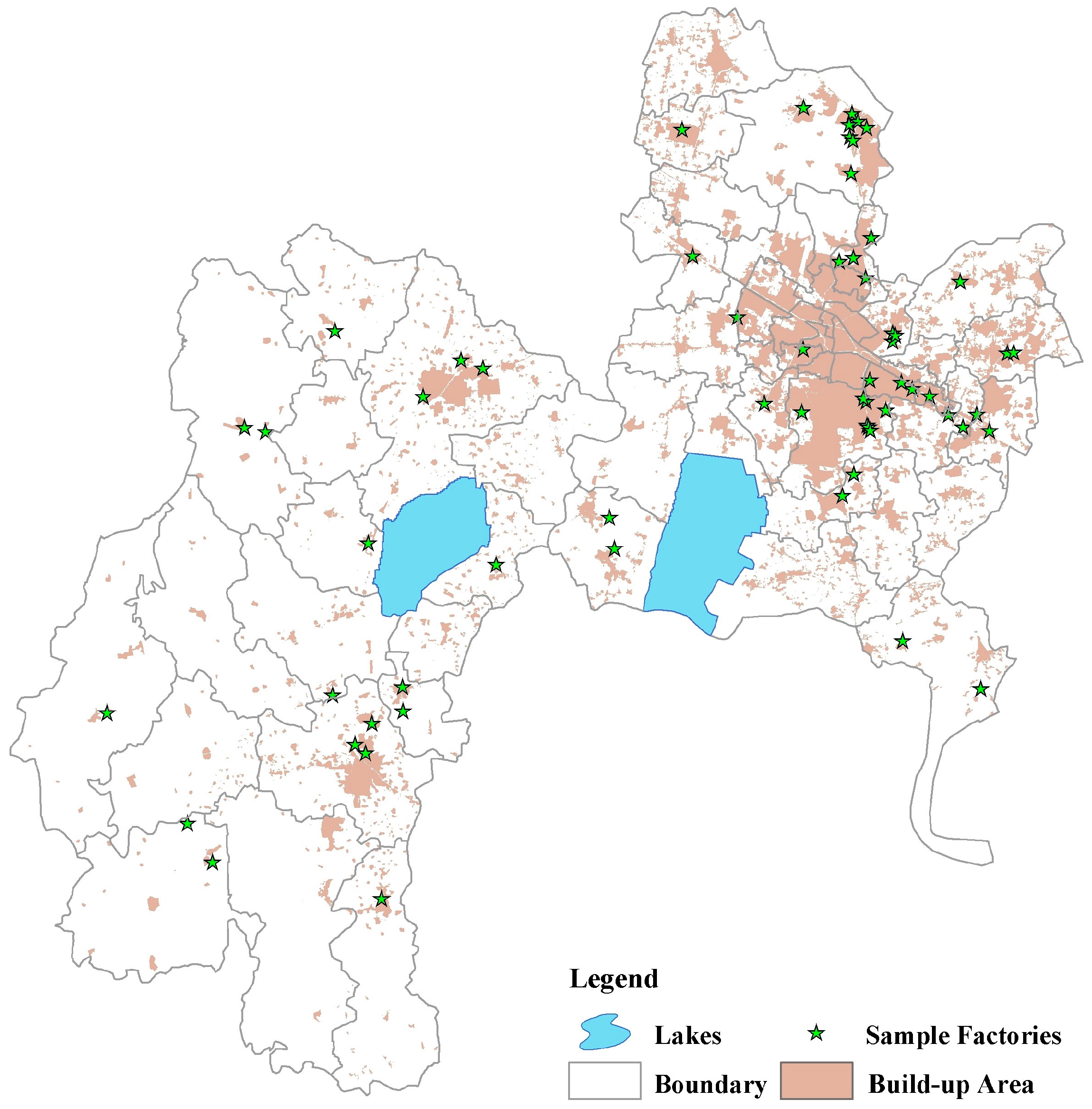
2.2. Measuring Recovery Capability
- : correct detection rate;
- : misdetection rate.
- : time consumption of ith sample monitoring point to return;
- : end time point of detected change of ith sample monitoring point;
- : end time point of downpour of ith sample monitoring point.
2.3. Connecting the Measurements of Recovery to Resilience
3. Results
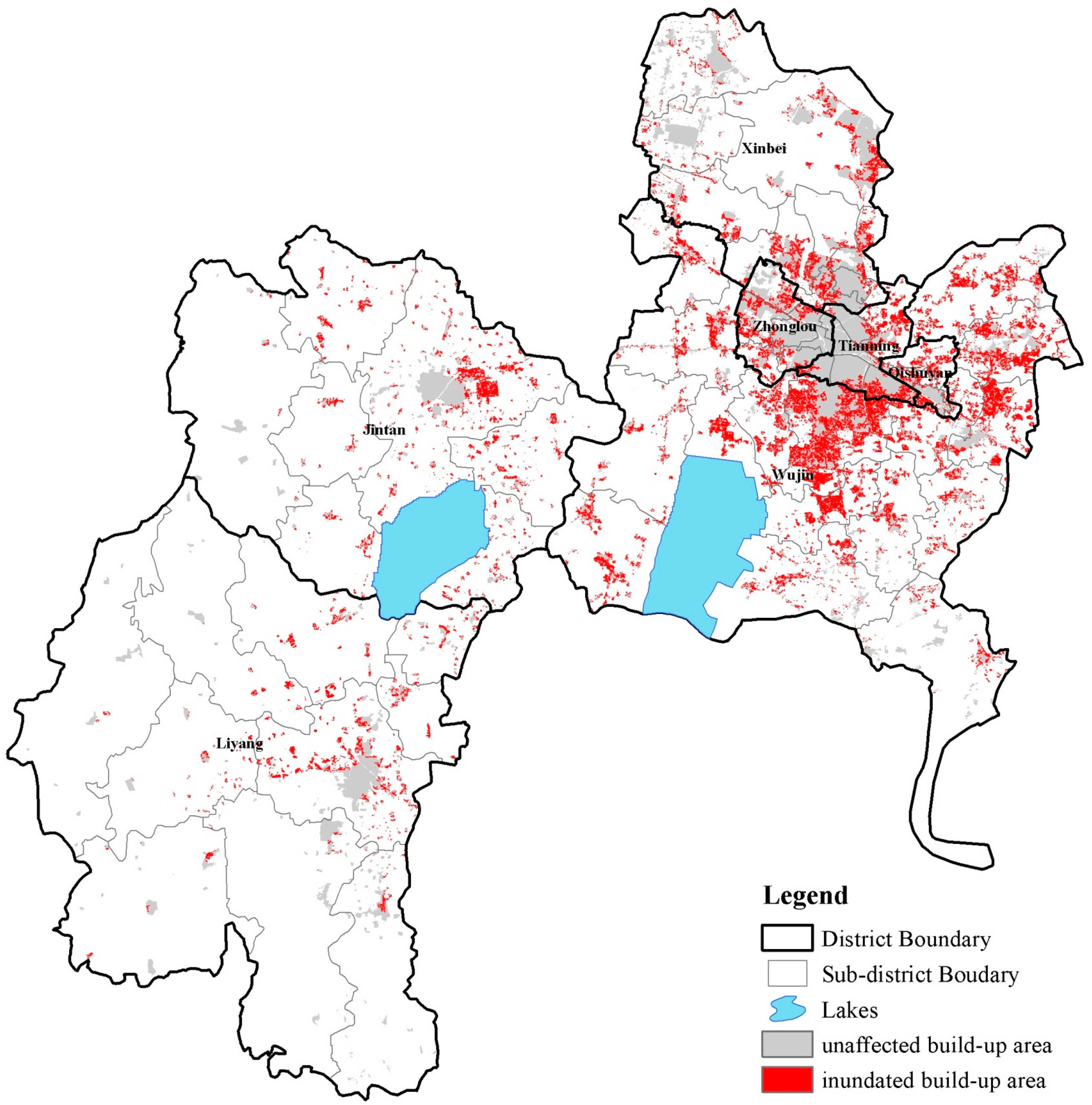
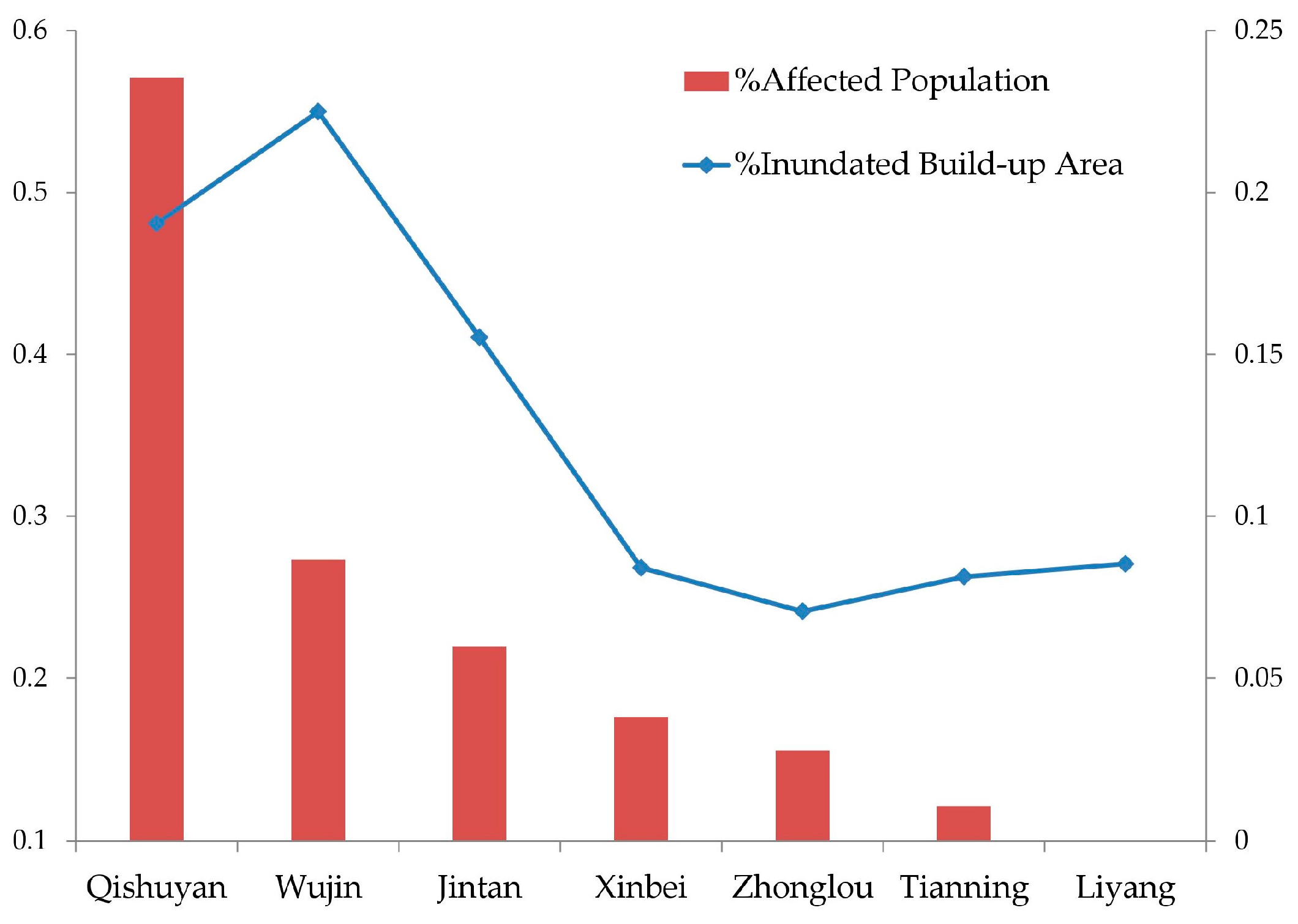
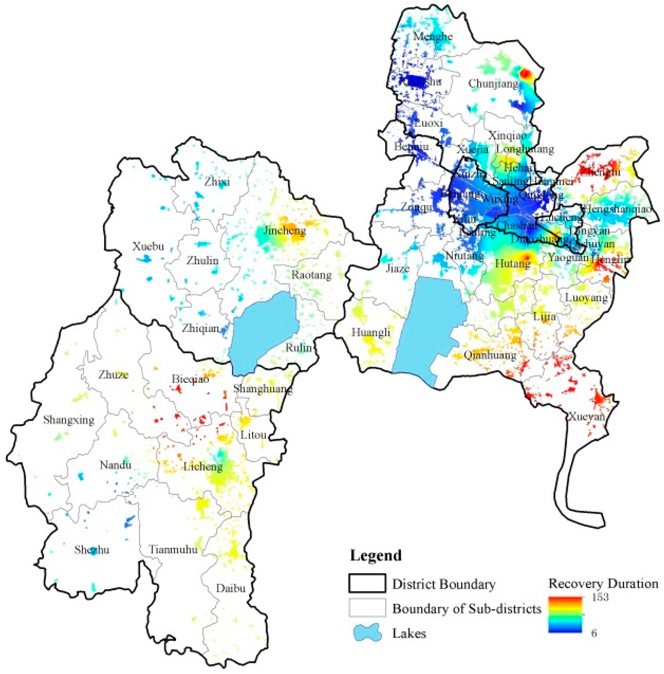
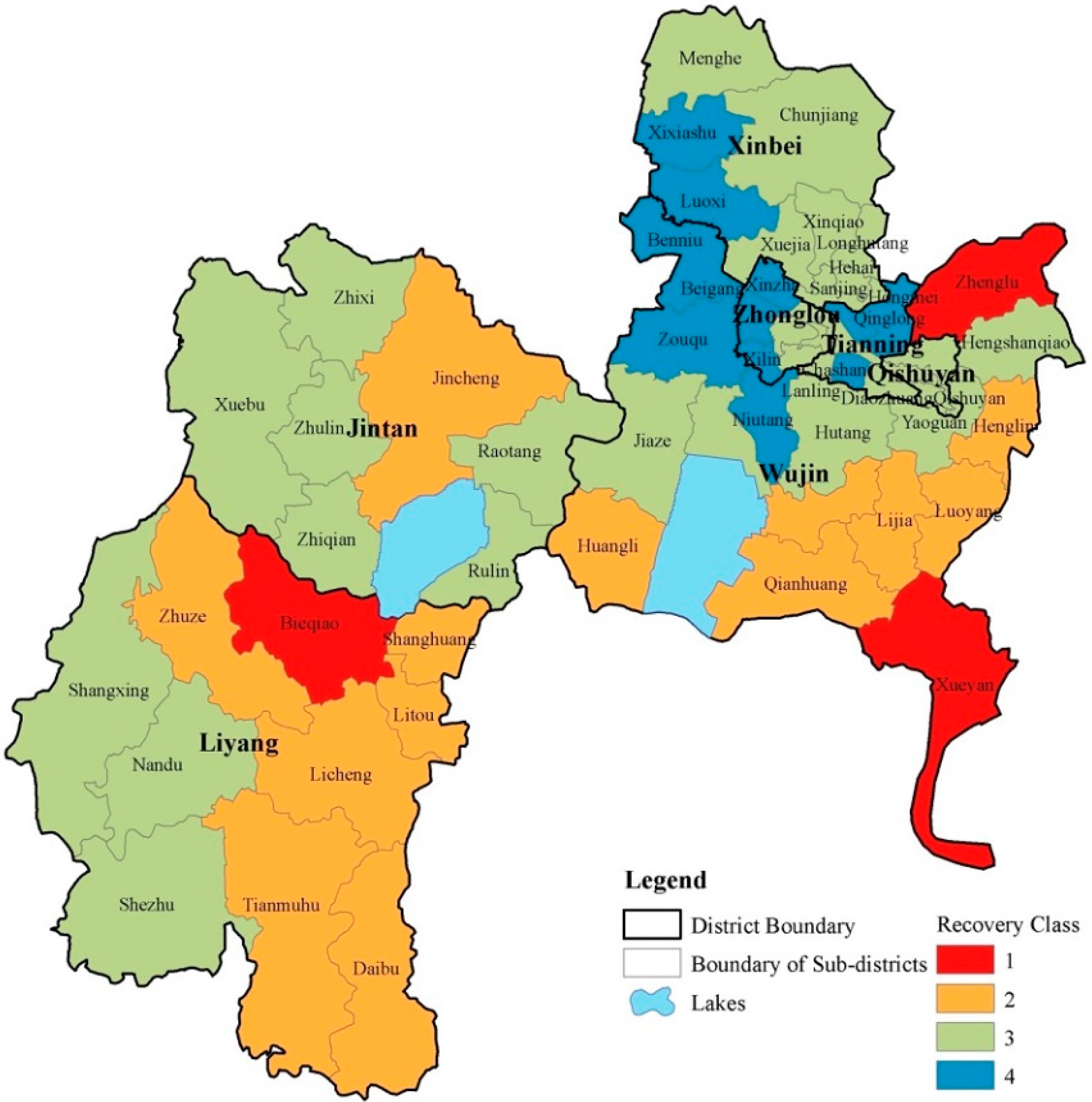
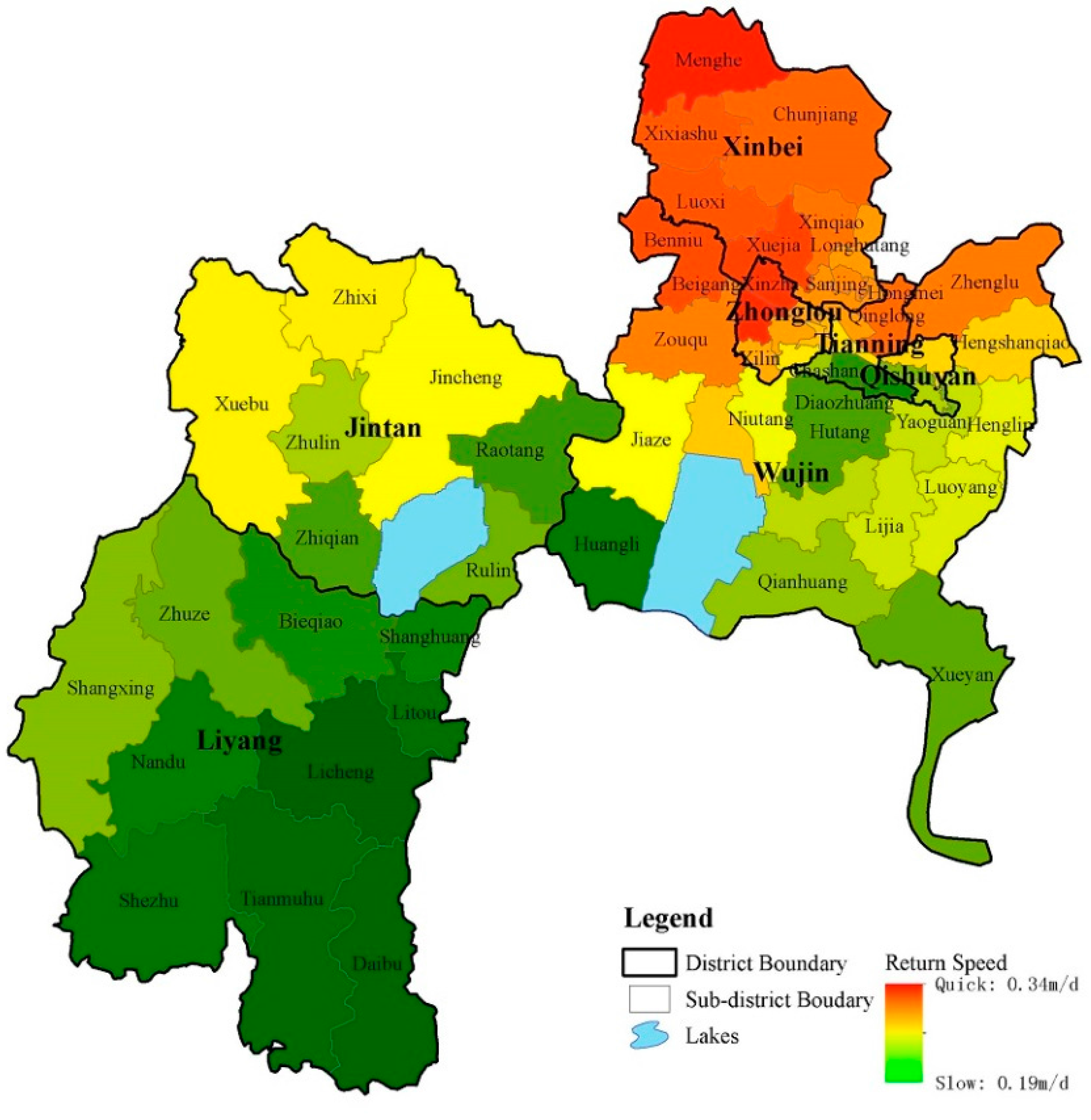
3.1. Results of Recovery Capability Measurements
3.2. Results of Regression Analysis
4. Conclusions and Discussion
Acknowledgments
Author Contributions
Conflicts of Interest
Appendix A
| Concepts | Disaster Resistance | Disaster Resilience |
|---|---|---|
| Definition |
|
|
| Context |
|
|
| Measures |
|
|
| Practical Examples |
|
|
|
| |
| Pros and Cons |
|
|
References
- Lo, A.Y.; Xu, B.; Chan, F.K.; Su, R. Social capital and community preparation for urban flooding in China. Appl. Geogr. 2015, 64, 1–11. [Google Scholar] [CrossRef]
- The Chinese Meteorological Administration. Meteorological Disaster Yearbook of China; Meteorological Press of China: Beijing, China, 2015. (In Chinese)
- Kobayashi, Y.; Porter, J.W. Flood Risk Management in the People’s Republic of China: Learning to Live with Flood Risk; Asian Development Bank: Manila, Philippines, 2012. [Google Scholar]
- Aerts, J.C.J.H.; Botzen, W.W.; Emanuel, K.; Lin, N.; de Moel, H.; Michel-Kerjan, E.O. Evaluating flood resilience strategies for coastal megacities. Science 2014, 344, 473–475. [Google Scholar] [CrossRef] [PubMed]
- Cox, L.A.T., Jr. Community resilience and decision theory challenges for catastrophic events. Risk Anal. 2012, 32, 1919–1934. [Google Scholar] [CrossRef] [PubMed]
- Rinne, P.; Nygren, A. From Resistance to Resilience: Media Discourses on Urban Flood Governance in Mexico. J. Environ. Policy Plan. 2015, 18, 4–26. [Google Scholar] [CrossRef]
- Bruneau, M.; Chang, S.E.; Eguchi, R.T.; Lee, G.C.; O’Rourke, T.D.; Reinhorn, A.M.; von Winterfeldt, D. A framework to quantitatively assess and enhance the seismic resilience of communities. Earthq. Spectra 2003, 19, 733–752. [Google Scholar] [CrossRef]
- Burton, C.G. A Validation of Metrics for Community Resilience to Natural Hazards and Disasters Using the Recovery from Hurricane Katrina as a Case Study. Ann. Assoc. Am. Geogr. 2015, 105, 67–86. [Google Scholar] [CrossRef]
- United Nations Development Program (UNDP). Disaster Resilience Measurements. 2014. Available online: http://www.preventionweb.net/files/37916_disasterresiliencemeasurementsundpt.pdf (accessed on 17 August 2017).
- United Nations Office for Disaster Risk Reduction (UNISDR). Disaster Resilience Scorecard for Cities. 2014. Available online: http://www.unisdr.org/2014/campaign-cities/Resilience%20Scorecard%20V1.5.pdf (accessed on 17 August 2017).
- Cutter, S.L.; Barnes, L.; Berry, M.; Burton, C.; Evans, E.; Tate, E.; Webb, J. A place-based model for understanding community resilience to natural disasters. Glob. Environ. Chang. 2008, 18, 598–606. [Google Scholar] [CrossRef]
- Joerin, J.; Shaw, R. Mapping climate and disaster resilience in cities. Community Environ. Disaster Risk Manag. 2011, 6, 47–61. [Google Scholar]
- Reams, M.A.; Lam, N.S.; Baker, A. Measuring capacity for resilience among coastal counties of the US Northern Gulf of Mexico Region. Am. J. Clim. Chang. 2012, 1, 194–204. [Google Scholar] [CrossRef] [PubMed]
- Cutter, S.L.; Ash, K.D.; Emrich, C.T. The geographies of community disaster resilience. Glob. Environ. Chang. 2014, 29, 65–77. [Google Scholar] [CrossRef]
- Yoon, D.K.; Kang, J.E.; Brody, S.D. A measurement of community disaster resilience in Korea. J. Environ. Plan. Manag. 2015, 59, 1–25. [Google Scholar] [CrossRef]
- Li, X.; Lam, N.; Qiang, Y.; Li, K.; Yin, L.; Liu, S.; Zheng, W. Measuring county resilience after the 2008 Wenchuan earthquake. Nat. Hazards Earth Syst. Sci. Discuss. 2015, 3, 81–122. [Google Scholar] [CrossRef]
- Vugrin, E.D.; Warren, D.E.; Ehlen, M.A. A resilience assessment framework for infrastructure and economic systems: Quantitative and qualitative resilience analysis of petrochemical supply chains to a hurricane. Process Saf. Prog. 2011, 30, 280–290. [Google Scholar] [CrossRef]
- Haynes, K.E.; Georgianna, T.D. Risk assessment of water allocation and pollution treatment policies in a regional economy: Reliability, vulnerability and resiliency in the Yellowstone Basin of Montana. Comput. Environ. Urban Syst. 1989, 13, 75–94. [Google Scholar] [CrossRef]
- Emergency Management Australia (EMA). The Australian Emergency Management Glossary. 1998. Available online: https://www.aidr.org.au/media/1430/manual-3-australian-emergency-management-glossary.pdf (accessed on 18 August 2017).
- Birkmann, J. Measuring Vulnerability to Natural Hazards: Towards Disaster Resilient Societies; No. 363.34 M484m; United Nations University Press: New York, NY, USA, 2006. [Google Scholar]
- Manyena, S.B. The concept of resilience revisited. Disasters 2006, 30, 434–450. [Google Scholar] [CrossRef] [PubMed]
- Fisher, R.E.; Bassett, G.W.; Buehring, W.A.; Collins, M.J.; Dickinson, D.C.; Eaton, L.K.; Haffenden, R.A.; Hussar, N.E.; Klett, M.S.; Millier, D.J.; et al. Constructing a Resilience Index for the Enhanced Critical Infrastructure Protection Program; No. ANL/DIS-10-9; Argonne National Laboratory (ANL): Lemont, IL, USA, 2010.
- Kates, R.W.; Colten, C.E.; Laska, S.; Leatherman, S.P. Reconstruction of New Orleans after Hurricane Katrina: A research perspective. Proc. Natl. Acad. Sci. USA 2006, 103, 14653–14660. [Google Scholar] [CrossRef] [PubMed]
- Olshansky, R.B.; Johnson, L.A.; Topping, K.C. Rebuilding communities following disaster: Lessons from Kobe and Los Angeles. Built Environ. 2006, 32, 354–374. [Google Scholar] [CrossRef]
- Zhang, Y. Modeling Single Family Housing Recovery after Hurricane Andrew in Miami-Dade County, FL. Ph.D. Thesis, Texas A&M University, College Station, TX, USA, 2006. [Google Scholar]
- Pendall, R.; Foster, K.A.; Cowell, M. Resilience and regions: Building understanding of the metaphor. Camb. J. Reg. Econ. Soc. 2009, 3, 71–84. [Google Scholar] [CrossRef]
- Fiksel, J. Designing resilient, sustainable systems. Environ. Sci. Technol. 2003, 37, 5330–5339. [Google Scholar] [CrossRef] [PubMed]
- Mayunga, J.S. Measuring the Measure: A Multi-Dimensional Scale Model to Measure Community Disaster Resilience in the US Gulf Coast Region. Ph.D. Thesis, Texas A&M University, College Station, TX, USA, 2009. [Google Scholar]
- Jordan, E.; Javernick-Will, A. Indicators of community recovery: Content analysis and Delphi approach. Nat. Hazards Rev. 2013, 14, 21–28. [Google Scholar] [CrossRef]
- Mileti, D.S. Disasters by Design: A Reassessment of Natural Hazards in the United States; Joseph Henry Press: Washington, DC, USA, 1999. [Google Scholar]
- Federal Emergency Management Agency (FEMA). Hazards, Disasters and U.S. Emergency Management: An Introduction, Appendix: Select Emergency Management-Related Terms and Definitions; FEMA: Washington, DC, USA, 2006.
- Phillips, B. Disaster Recovery; Auerbach Publications: Boca Raton, FL, USA, 2009. [Google Scholar]
- Chang, S.E. Urban disaster recovery: A measurement framework and its application to the 1995 Kobe earthquake. Disasters 2010, 34, 303–327. [Google Scholar] [CrossRef] [PubMed]
- Mieler, M.; Stojadinovic, B.; Budnitz, R.; Comerio, M.; Mahin, S. A framework for linking community-resilience goals to specific performance targets for the built environment. Earthq. Spectra 2015, 31, 1267–1283. [Google Scholar] [CrossRef]
- Brown, D.; Platt, S.; Bevington, J. Disaster Recovery Indicators; Cambridge University Centre for Risk in the Build Environment (CURBE): Scroope Terrace, Cambridge, UK, 2010. [Google Scholar]
- Olshansky, R.B. Toward a Theory of Community Recovery from Disaster: A Review of Existing Literature. Presented at the 1st International Conference of Urban Disaster Reduction, Kobe, Japan, 18–20 January 2005. [Google Scholar]
- Tierney, K.; Oliver-Smith, A. Social Dimensions of Disaster Recovery. Int. J. Mass Emerg. Disasters 2012, 30, 123–146. [Google Scholar]
- Gall, M. From Social Vulnerability to Resilience: Measuring Progress Toward Disaster Risk Reduction; UNU-EHS: Bonn, Germany, 2013. [Google Scholar]
- National Research Council (NRC). Disaster Resilience: A National Imperative; National Academies Press: Washington, DC, USA, 2012. [Google Scholar]
- United Nations Framework Convention on Climate Change (UNFCCC). Current Knowledge on Relevant Methodologies on Data Requirements as Well as Lessons Learned and APS Identified at Different Levels, in Assessing the Risk of Loss and Damage Associated with the Adverse Effects on Climate Change. 2012. Available online: http://unfccc.int/resource/docs/2012/tp/01.pdf (accessed on 17 August 2017).
- Ma, B. Changzhou Watching a Record-Breaking Precipitation during the Last 24 Hours. Yangtse Evening, 27 June 2015. Available online: http://china.huanqiu.com/article/2015-06/6789103.html (accessed on 18 August 2017). (In Chinese).
- Tan, M. 24 Hours Precipitation in Changzhou in Jiangsu Province Ranking the First in China. China Daily, 29 June 2015. Available online: http://www.chinadaily.com.cn/hqcj/xfly/2015-06-29/content_13899607.html (accessed on 17 August 2017). (In Chinese).
- Muggeo, V.M.; Adelfio, G. Efficient change point detection for genomic sequences of continuous measurements. Bioinformatics 2010, 27, 161–166. [Google Scholar] [CrossRef] [PubMed]
- Matteson, D.S.; James, N.A. A nonparametric approach for multiple change point analysis of multivariate data. J. Am. Stat. Assoc. 2014, 109, 334–345. [Google Scholar] [CrossRef]
- Allen, D.E.; Kalev, P.S.; McAleer, M.J.; Singh, A.K. Nonparametric Multiple Change-Point Analysis of the Responses of Asian Markets to the Global Financial Crisis. In Handbook of Asian Finance: REITs, Trading, and Fund Performance; Elsevier: Amsterdam, The Netherlands, 2014; Volume 2, p. 267. [Google Scholar]
- Schmaljohann, H.; Kämpfer, S.; Fritzsch, A.; Kima, R.; Eikenaar, C. Start of nocturnal migratory restlessness in captive birds predicts nocturnal departure time in free-flying birds. Behav. Ecol. Sociobiol. 2015, 69, 909–914. [Google Scholar] [CrossRef]
- Ross, G.J. Parametric and nonparametric sequential change detection in R: The cpm package. J. Stat. Softw. 2015, 66. [Google Scholar] [CrossRef]
- Killick, R.; Eckley, I. Changepoint: An R package for changepoint analysis. J. Stat. Softw. 2014, 58, 1–19. [Google Scholar] [CrossRef]
- James, N.A.; Matteson, D.S. ecp: An R package for nonparametric multiple change point analysis of multivariate data. J. Stat. Softw. 2014, 62. [Google Scholar] [CrossRef]
- Ban, Y.; Li, S. China: Open access to earth land-cover map. Nature 2014, 514, 434. [Google Scholar] [CrossRef]
- Jordan, E.; Javernick-Will, A.; Tierney, K. Post-tsunami recovery in Tamil Nadu, India: Combined social and infrastructural outcomes. Nat. Hazards 2016, 84, 1327–1347. [Google Scholar] [CrossRef]
- Jamil, S.; Amul, G.G. Community Resilience and Critical Urban Infrastructure: Where Adaptive Capacities Meet Vulnerabilities; Center for Non-Traditional Security Studies—NTS Insights: Singapore, 2013. [Google Scholar]
- Cutter, S.L. The landscape of disaster resilience indicators in the USA. Nat. Hazards 2016, 80, 741–758. [Google Scholar] [CrossRef]
- Cutter, S.L.; Boruff, B.J.; Shirley, W.L. Social vulnerability to environmental hazards. Soc. Sci. Quart. 2003, 84, 242–261. [Google Scholar] [CrossRef]
- Cutter, S.L.; Director, H. A Framework for Measuring Coastal Hazard Resilience in New Jersey Communities; White Paper for the Urban Coast Institute: West Long Branch, NJ, USA, 2008. [Google Scholar]
- Wood, N.J.; Burton, C.G.; Cutter, S.L. Community variations in social vulnerability to Cascadia-related tsunamis in the US Pacific Northwest. Nat. Hazards 2010, 52, 369–389. [Google Scholar] [CrossRef]
- Liao, K.H. A Theory on Urban Resilience to Floods—A Basis for Alternative Planning Practices. Ecol. Soc. 2012, 17, 388–395. [Google Scholar] [CrossRef]
- Wang, S.H.; Huang, S.L.; Budd, W.W. Resilience analysis of the interaction of between typhoons and land use change. Landsc. Urban Plan. 2012, 106, 303–315. [Google Scholar] [CrossRef]
- Sun, H.; Cheng, X.; Dai, M. Regional flood disaster resilience evaluation based on analytic network process: A case study of the Chaohu Lake Basin, Anhui Province, China. Nat. Hazards 2016, 82, 39–58. [Google Scholar] [CrossRef]
- Frazier, T.G.; Thompson, C.M.; Dezzani, R.J.; Butsick, D. Spatial and temporal quantification of resilience at the community scale. Appl. Geogr. 2013, 42, 95–107. [Google Scholar] [CrossRef]
- Cai, H.; Lam, N.S.N.; Zou, L.; Qiang, Y.; Li, K. Assessing community resilience to coastal hazards in the Lower Mississippi River Basin. Water 2016, 8, 46. [Google Scholar] [CrossRef]


| Sample Cases | Change | Non-Change |
|---|---|---|
| Damage | a | b |
| Non-Damage | c | d |
| Sub-Component | Label | Variable | Measures | Data Source |
|---|---|---|---|---|
| Social Component | Age Distribution | Age | % population between 15 and 64 years old | PCC, 2010 |
| Sex Ratio | Gender | sex ratio (male/female) | PCC, 2010 | |
| Health Services | Support of health facilities | population share of health facilities | PCC, 2010 | |
| Non-household Population | Mobility of labor force | % non-household population | PCC, 2010 | |
| Economic Component | Ratio of Urban to Rural | Urban population | ratio of residents to villages | OSM, 2013 |
| GDP per Capita | Gross Domestic Product | Gross Domestic Product per capita | GCRD, 2010 | |
| Share of CBD | Commercial establishment | Share of business (CBD centers) within build-up area | OSM, 2013 | |
| Manufacturing Density | Manufacturing establishment | density of manufacturing within build-up area | OSM, 2013 | |
| Infrastructural Component | Road Density | Transport | road density | OSM, 2013 |
| Access to Open Space | Emergency preparation | access to open space (parks, urban green space, stadium, parking area) | OSM, 2013 | |
| Access to Administration | Emergency preparation | access to governmental institutions (administration center, police station) | OSM, 2013 | |
| Access to Hospital | Emergency preparation | access to hospitals | OSM, 2013 | |
| Environmental Component | DEM | Geological condition | mean of Digital Elevation Model (DEM) data | GDEMV2, 2009 |
| Slope | Geological condition | mean slope | GDEM SLOPE, 2009 | |
| River Density | Land use in natural terms | density of water network | OSM, 2013 | |
| Urban Green Area | Green area within build-up area | total area of green space per square kilometer of build-up area | OSM, 2013 |
| Mvc | Change | Non-Change |
| Damage | 28 | 18 |
| Non-Damage | 3 | 8 |
| Cpm | Change | Non-Change |
| Damage | 35 | 12 |
| Non-Damage | 8 | 2 |
| Ecp | Change | Non-Change |
| Damage | 35 | 11 |
| Non-Damage | 5 | 6 |
| Measure | mvc | cpm | ecp |
|---|---|---|---|
| Correct Detection Rate | 0.63 | 0.65 | 0.72 |
| Misdetection Rate | 0.37 | 0.35 | 0.28 |
| Component | Variable | Estimate | Significance (Two-Tailed) |
|---|---|---|---|
| Social | Sex Ratio | 1.074 | 0.050 * |
| Health Service | 1.219 | 0.043 * | |
| Economic | Ratio of Urban to Rural | 1.393 | 0.044 * |
| Share of CBD | — | — | |
| Infrastructural | Road Density | 3.009 | 0.003 ** |
| Access to Open Space | 2.537 | 0.002 ** | |
| Environmental | Slope | 1.176 | 0.014 * |
| River Density | 0.934 | 0.092 | |
| Urban Green Area | — | — | |
| Control | Return Speed of Water Level | 1.053 | 0.010 ** |
© 2017 by the authors. Licensee MDPI, Basel, Switzerland. This article is an open access article distributed under the terms and conditions of the Creative Commons Attribution (CC BY) license (http://creativecommons.org/licenses/by/4.0/).
Share and Cite
Song, J.; Huang, B.; Li, R. Measuring Recovery to Build up Metrics of Flood Resilience Based on Pollutant Discharge Data: A Case Study in East China. Water 2017, 9, 619. https://doi.org/10.3390/w9080619
Song J, Huang B, Li R. Measuring Recovery to Build up Metrics of Flood Resilience Based on Pollutant Discharge Data: A Case Study in East China. Water. 2017; 9(8):619. https://doi.org/10.3390/w9080619
Chicago/Turabian StyleSong, Jinglu, Bo Huang, and Rongrong Li. 2017. "Measuring Recovery to Build up Metrics of Flood Resilience Based on Pollutant Discharge Data: A Case Study in East China" Water 9, no. 8: 619. https://doi.org/10.3390/w9080619
APA StyleSong, J., Huang, B., & Li, R. (2017). Measuring Recovery to Build up Metrics of Flood Resilience Based on Pollutant Discharge Data: A Case Study in East China. Water, 9(8), 619. https://doi.org/10.3390/w9080619


