A Probabilistic Short-Term Water Demand Forecasting Model Based on the Markov Chain

Abstract

This paper proposes a short-term water demand forecasting method based on the use of the Markov chain. This method provides estimates of future demands by calculating probabilities that the future demand value will fall within pre-assigned intervals covering the expected total variability. More specifically, two models based on homogeneous and non-homogeneous Markov chains were developed and presented. These models, together with two benchmark models (based on artificial neural network and naïve methods), were applied to three real-life case studies for the purpose of forecasting the respective water demands from 1 to 24 h ahead. The results obtained show that the model based on a homogeneous Markov chain provides more accurate short-term forecasts than the one based on a non-homogeneous Markov chain, which is in line with the artificial neural network model. Both Markov chain models enable probabilistic information regarding the stochastic demand forecast to be easily obtained.

1. Introduction

Water distribution systems fulfil the fundamental task of satisfying the water demand of users, and their long-term and short-term management can be supported by the use of water demand forecasting models. In fact, for the purpose of activities related to the design, maintenance and upgrading of water supply networks (e.g., expansion of distribution systems or replacement of parts of networks), which entail long-term planning, it is fundamental to have an accurate estimate of monthly or yearly demand in the years to come, that is, over the useful lifetime of the installation. Analogously, forecasts of daily or hourly demands over limited time horizons (for example a week or the next 24 h) can provide useful information for planning short-term or real-time management of the devices at the service of water distribution systems, such as the planning of pumping station operations, the control of valves, etc.

Depending on their features, water demand forecasting models can be divided into different categories. A first distinction can be made, in relation to the different practical objectives just mentioned, based on the forecasting frequency and the time horizon (i.e., the length of future time interval the forecast is intended to cover) (see [1]). In this work, the attention is focussed on short-term demand forecasting models, which generally predict hourly or sub-hourly demands over a time horizon normally ranging between 6 and 48 h [2,3,4,5,6].

A further distinction can be made in relation to the adopted modelling technique. Various water demand forecasting models based on data-driven techniques, in particular artificial neural networks (ANN), have recently been proposed [3,7,8,9,10,11,12,13,14]. A different approach to demand forecasting is based on the representation of periodic behaviours that typically characterise water demands. It is in fact possible to recognise trends or patterns, which are generally influenced by seasonality, climate conditions and the types and habits of the users served by the system. The structure of various water demand forecasting models is based precisely on the description of such behaviours [4], possibly in conjunction with techniques of time series analysis such as autoregressive processes [2], or Markov processes [15]. Most of the above techniques, especially the forecasting models based on ANN and similar methods, fall into the category of black box models (as opposed to white box models, such as physically-based models). Whilst accurate, black box models are simply not transparent in terms of mapping inputs (past demands and different explanatory factors) onto outputs (forecasted demands). The water demand forecasting model proposed here falls into the category of grey box-type models, i.e., with limited but better transparency when compared with black box models.

Finally, it is possible to formulate a further distinction between forecasting models based on the type of results they furnish. Water demand forecasting is characterised by a certain degree of uncertainty, due to the natural variability of the water consumption. Quantification/characterisation of this natural variability is very important in the planning or management of water distribution systems [16]. The models can therefore be classified into deterministic models, which provide a deterministic estimate of future water demands, and models that also provide an estimate of the stochastic behaviour of the demand forecast. Most models proposed in the scientific literature, including the ones mentioned thus far, belong to the former category, whereas the latter category embraces less recently proposed models, such as the Bayesian-based models [17,18,19,20,21,22], the approach proposed by Alvisi and Franchini [16] based on the use of the Model Conditional Processor [23], and the approach proposed by Cutore et al. [24], based on a neural network trained by means of the SCEM-UA algorithm [25]. All in all, stochastic models should be preferred to deterministic ones, due to additional information provided about the forecasted demands. However, existing stochastic forecasting models can be very computationally demanding, as they tend to use Monte Carlo simulations to assess the probability distribution of the future demand value and the related prediction bounds.

In this paper, a new approach for short-term water demand forecasting based on the statistical concept of the Markov chain (grey box modelling approach) is proposed. The model is capable of providing both a deterministic forecast of the future values of water demand, and a characterisation of the stochastic behaviour of the forecasted values (at reduced computational effort compared to most of the existing methods). The model, applied with the aim of estimating future hourly demands over a time horizon of 24 h relying solely on observed water demand data, is characterised by a simple structure, easy to comprehend and control.

The Markov chain technique is outlined in Section 2 below where, after giving the theoretical basis, the developed models are then illustrated. In Section 3, the case studies the models were applied to, and the benchmark models used by way of comparison, are described. After analysing and comparing the results obtained from the application of the Markov models and the benchmark models in Section 4, the final conclusions are presented in Section 5.

2. Markov Chain Based Demand Forecasting

2.1. Overview

The proposed approach is based on the statistical concept of the Markov Chain (MC) and aims to forecast short-term water demand while characterising the demand’s stochastic behaviour. In the scientific literature, various examples of forecasting models applying this concept can be found, both in the context of water demands [15], and in other engineering contexts such as in the prediction of the performance of bridge decks [26], traffic flow forecasting [27], wind power forecasting [28] and streamflow forecasting for the prediction of flood events [29]. In particular, in the context of water demand, proposed by Shvarster et al. [15] propose an hourly water demand forecasting model in which each day is divided into three parts, referred to as “rising”, “oscillating”, and “falling” segments. Within each segment, the water demand is modelled with a third-order autoregressive process. The transition from one segment to the next is modelled with a Markov process.

The approach proposed here, by contrast, exploits the Markov chain concept to characterise the probability that the demand in one or more successive times (for example, in the next hour or in the next 2, 3, … hours) will fall into an assigned interval, where the interval at the current time step is known. In the sections that follow, the Markov chain concept is illustrated, and then its application to water demand forecasting is described.

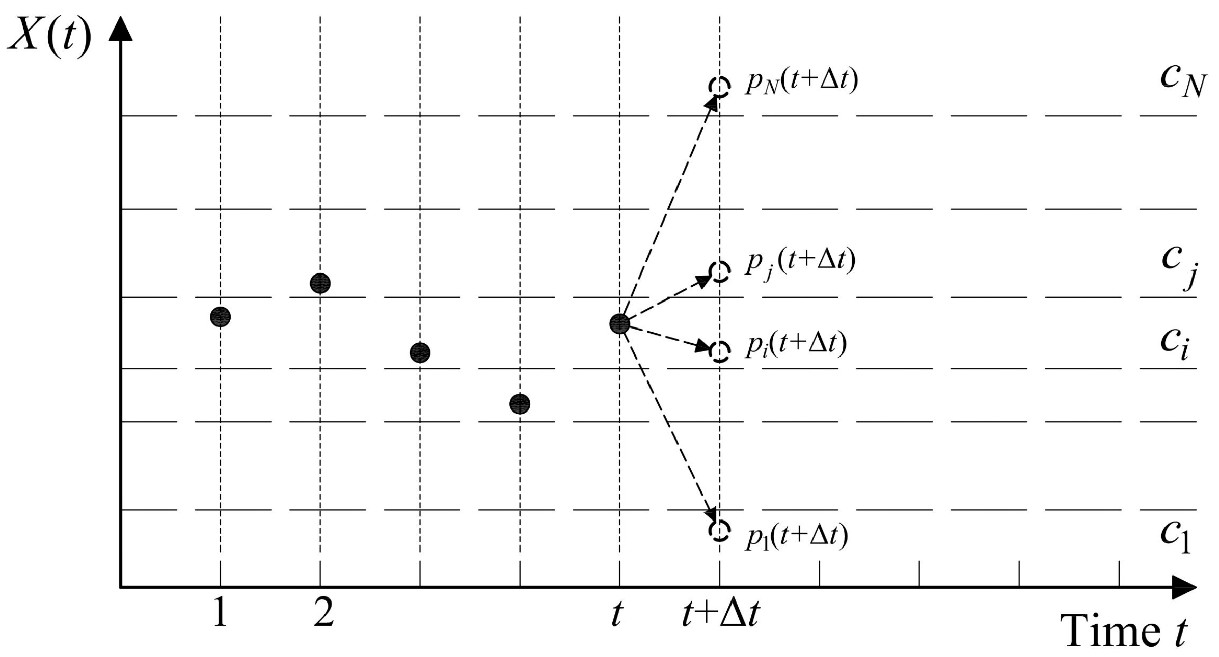
2.2. The Markov Chain

A statistical process, i.e., the succession of a random variable X(t), with $t\in T$, may be considered a Markov process if it exploits the Markov theorem [30]. Let us assume that the domain T of the variable t is the time, divided in discrete intervals ∆t, and that the domain of existence of the variable X(t) is known and divided into N intervals, each of which is defined as a class c_i (with i = 1,.., N) of the process (see Figure 1).

The probability p_i(t) that, at a generic time t, the process will be in a generic class c_i, can be defined as:

$$p_i(t)=\mathrm{Pr}[X(t)\in c_i],$$

(1)

The generic p_i(t) represents the i-th component of the row-vector p(t) = [p₁(t), p₂(t),…, p_N(t)], which contains all the probabilities that the process is at the generic time t in each of the N classes. Of course, it results ${\displaystyle \sum _{i=1}^N{p}_i(t)=1}$ for every t.

In passing from a class c_i at time t to a class c_j at the next time t + ∆t, the process undergoes a transition, which is associated with a probability π_ij(t), called transition probability. The probabilities associated with every possible transition from t to t + ∆t are the components making up the transition matrix $\Pi (t)\in {\square }^{NxN}$:

$$\Pi (t)=\left[\begin{array}{cccccc}{\pi }_{11}(t)& \dots & {\pi }_{1i}(t)& {\pi }_{1j}(t)& \dots & {\pi }_{1N}(t)\\ \dots & \dots & \dots & \dots & \dots & \dots \\ {\pi }_{i1}(t)& \dots & {\pi }_{ii}(t)& {\pi }_{ij}(t)& \dots & {\pi }_{iN}(t)\\ {\pi }_{j1}(t)& \dots & {\pi }_{ji}(t)& {\pi }_{jj}(t)& \dots & {\pi }_{jN}(t)\\ \dots & \dots & \dots & \dots & \dots & \dots \\ {\pi }_{N1}(t)& \dots & {\pi }_{Ni}(t)& {\pi }_{Nj}(t)& \dots & {\pi }_{NN}(t)\end{array}\right],$$

(2)

where every row of the matrix Π(t) corresponds to the starting class of the process, and every column to the class of arrival: for instance, the probability π_ij(t) of belonging in class c_j at time t + ∆t starting from class c_i at the preceding time t, is placed in the i-th row and j-th column of the matrix.

It should be noted that the transition matrix Π(t) can vary at every step of the process, and this behaviour is generally indicated as a non-homogeneous Markov chain. A homogeneous Markov chain is based, by contrast, on the assumption that the transition probability is independent of t. This condition implies the existence of a single transition matrix, Π, which remains constant with variations in t and is characteristic of the entire process.

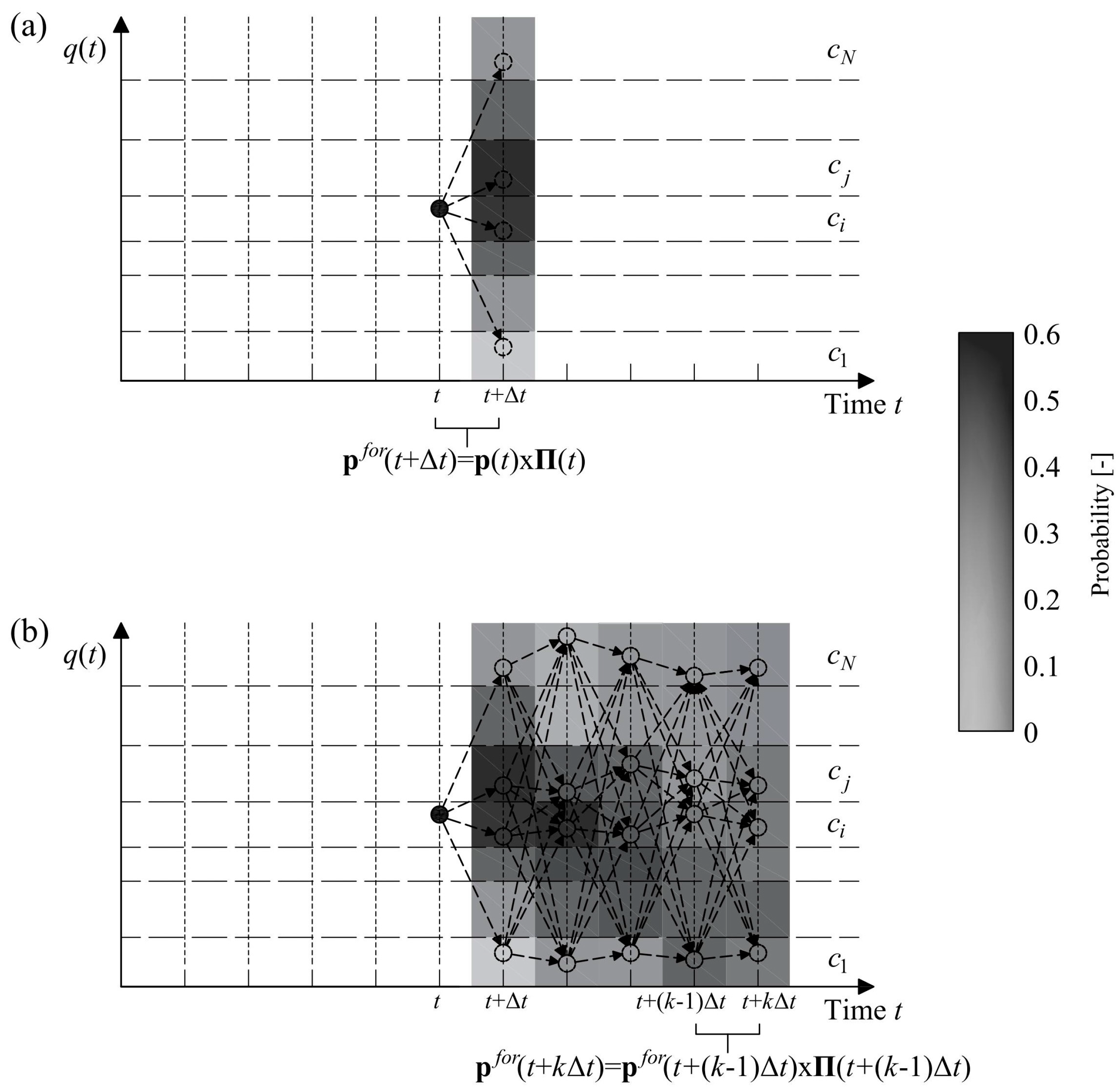
The transition matrix characterises the Markov process itself, since it quantifies the tendency of the process to move from one class to another in two successive times. With the transition matrix of a certain Markov process being known, the Markov chain theory allows the estimation of the probability that the process has to belong to each class one time ahead of the current one (for example in t + ∆t when t is the current time). In particular, in a real-time forecasting framework, with t being the current time, p(t) the corresponding probability vector of the process and Π(t) the correspondent transition matrix, the probability vector of the process at time t + ∆t, p^for(t+∆t), can be estimated as:

$$p^{for}(t+\Delta t)=p(t)\times \Pi (t),$$

(3)

This estimation is displayed in Figure 2a showing, at the time step centered in t + ∆t, each class coloured with a shade of grey, correspondent to the calculated probability. More in general, by triggering a Markov chain and exploiting, for every time lag k following the first, the forecast made for the preceding times, it is possible to extend the time horizon to k∆t ahead (with k > 1), i.e.,:

$$p^{for}(t+k\Delta t)=p^{for}(t+(k-1)\Delta t)\times \Pi (t+(k-1)\Delta t) \mathrm{with} k>1,$$

(4)

What has been illustrated thus far can be used to obtain probability vectors at every time t + k∆t, one for every time lag k (with k = 1,…, K) (see Figure 2b); these vectors characterise, for every time lag, the probability that the process will fall into each of the N classes.

The proposed Markov chain method exploits this concept in order to provide stochastic and deterministic forecasts of water demand, as detailed in the next section.

2.3. Demand Forecasting Model

The proposed water demand forecasting model is based on the assumption that the trend in water demand can be defined as a Markov process. Generally speaking, it can be assumed that the random variable of the process at the time t can be identified with the mean water demand q(t) in the generic time interval Δt (for example, Δt = 1 h). Moreover, it is possible to identify N classes c₁,c₂,…, c_N into which the entire range of variability of the water demand can be divided.

If the state, i.e., the class c_i, of the water demand at the current time t and the transition matrix referred to t are known, the Markov chain allows us to define what its state in the future Δt will be in probabilistic terms. In fact, Equation (3) can be used to estimate the probability vector p^for(t + Δt), where p(t) is referred to a real observed value, being in a context of real-time application of the model, thus composed of N − 1 null values and a value of 1 correspondent to the class the demand q(t) belongs to. As regards the transition matrix, it represents a parameter of the model that can be estimated on the basis of the observed water demands used in the model calibration phase, as detailed below. Since it is a calibrated variable, it will be henceforth indicated as $\widehat{\Pi }(t)$. The forecast can be tied up to kΔt ahead using Equation (4), thus estimating the probabilities of the demand to fall within each class at the time t + kΔt, p^for(t + kΔt), using the estimate made one time earlier and the correspondent transition matrix.

This information can also be used to obtain a deterministic forecast of future water demand q^for (t + k∆t) at a generic time t + kΔt in the following manner [28].

A weighted average of the N central values of the classes c_i (with i = 1,…, N), represented in the vector m = [m₁, m₂,…, m_N], is computed using the components $p_i^{for}(t+k\Delta t)$(with i = 1,.., N) of the probability vector predicted for the time t + kΔt as weights:

$$q^{for}(t+k\Delta t)={\displaystyle \sum _{i=1}^N{m}_i\cdot p_i^{for}(t+k\Delta t)} ,$$

(5)

At this point it is important to set forth some considerations regarding the advisability of adopting a non-homogeneous or homogeneous Markov chain to predict the vector p^for(t + k∆t) in the case of short-term water demands (for example, to obtain hourly water demand forecasts for the next K = 24 h). Water demands are generally characterised by periodic patterns, present on different time scales. Considering, for example, the hourly water demands over the course of a day, it is possible to observe that they follow a trend or pattern that tends to reflect the type and the habits of the users served. In the case of residential users, the demand trends show morning and evening peaks, reduced demand during the night and variable demand in the afternoon hours; water use may also differ depending on whether it is a weekday or a holiday [2]. In the trends in demand over time, it is thus possible to distinguish different phases—rising, falling, etc.—characterised by a probability of demand transitioning from one class to another, which will clearly vary from phase to phase. As we are dealing with a time series characterised by periodic patterns, it would seem appropriate to use an approach based on a non-homogeneous Markov chain. On the other hand, prior to the application of the model, the demand time series could be suitably normalised (brought to a mean of zero and unit variance), thus creating the conditions for the use of an approach based on a homogeneous Markov chain.

Two different formulations of the model based respectively on the use of a non-homogeneous Markov chain (NHMC) and a homogeneous Markov chain (HMC), were developed on the basis of these considerations as detailed below.

2.3.1. Non-Homogeneous Markov Chain (NHMC) Model

In this first case, it is assumed to work directly on the water demand time series q(t) and, given their periodic nature, to adopt a non-homogeneous Markov chain in order to take into account that the transition probability (and hence the transition matrix) varies as a function of time. In fact, given that, as mentioned earlier, the demand patterns generally show rising and falling phases during the day, each of them can be characterised by a different behaviour of the Markov process, in terms of transitions between classes. In the rising phases, for example, it should be more likely to see demands transition, in two consecutive instances, toward a higher class than the starting one, or at least remain in the same class. There is a reduced probability of observing demands transition to a lower class than the starting one. The opposite applies for the falling phases.

Assuming, moreover, that each of the phases making up the demand pattern over the course of the day is characterised by a single transition matrix, it is thus necessary to identify the F time ranges f₁,f₂,…, f_F, corresponding to the different rising and falling phases of the pattern. Incidentally, the assumption that each phase is characterised by a single transition matrix implies that the process is described through a sort of sequence of different homogeneous Markov processes.

From an operational viewpoint, the F time phases can be identified by making reference to the average trend in demand over the course of a day, possibly distinguishing between working and non-working days. Therefore, for the various phases f₁, f₂,…, f_F, the corresponding transition matrices ${\widehat{\Pi }}_{f_1},{\widehat{\Pi }}_{f_2},\dots ,{\widehat{\Pi }}_{f_F}$can be estimated, using the observed calibration data. An estimation of the generic component ${\widehat{\pi }}_{f_w,ij}$ (with w = 1,…, F and i,j = 1,…, N) of the transition matrix ${\widehat{\Pi }}_{f_w}$ is made, during the model calibration phase, by counting the transitions from c_i to c_j (with i,j = 1,…, N) between successive pairs of times, for which the starting time belongs to the phase f_w, and then dividing by the total transitions for which the starting time is inside the phase f_w, and which have the class c_i as the starting class, i.e.:

$${\widehat{\pi }}_{f_w,ij}=\frac{n_{f_w,ij}}{{\displaystyle \sum _{j=1}^N{n}_{f_w,ij}}} \mathrm{with} i,j=1,\dots ,N , w=1,\dots ,F ,$$

(6)

where $n_{f_w,ij}$ indicates the number of transitions from class c_i to class c_j in the consecutive times for which the starting time is inside the phase f_w. It is necessary to highlight that as the number of F phases increases, the accuracy of the estimate of the transition matrices will tend to decrease, because the number of data available for the purpose of the estimate decreases. Therefore, the number of the F phases adopted should not depend only on the trend in demand, but should also take into account the number of observed data available for calibrating the model.

During the actual application of the model, the forecast at a time lag 1, from the generic time t, to the time t + Δt is made using the transition matrix ${\widehat{\Pi }}_{f_w}$associated with the phase f_w, in which the starting time t falls, i.e.:

$$p^{for}(t+\Delta t)=p(t)\times {\widehat{\Pi }}_{f_w} \mathrm{with} t\in f_w,$$

(7)

while for time lags larger than one, the model is based on the following equation:

$$p^{for}(t+k\Delta t)=p^{for}(t+(k-1)\Delta t)\times {\widehat{\Pi }}_{f_w} \mathrm{with} (t+(k-1)\Delta t)\in f_w,$$

(8)

In practical terms, therefore, in the event that the set of kΔt data forecasted by the model at a generic time t straddles two different phases, the transition matrix used to estimate the vector p^for at the different time lags will change. The transition matrix used for each forecast will be “moving” with the forecast, instead of being fixed and equal to the one correspondent to t (i.e., the start time of the forecast). Thus, for every time lag k, the water demand of the generic time t + kΔt, which is based on the forecast made one time earlier t + (k − 1)Δt, will be estimated basing on the transition matrix associated with the phase the time t + (k − 1)Δt belongs to (rather than being based on the one correspondent to the time t).

2.3.2. Homogeneous Markov Chain (HMC) Model

The second formulation of the Markov demand forecasting model is based on the application of a homogeneous Markov chain to a duly transformed demand time series. It may be noted, in fact, that in the case of a homogeneous Markov chain, the probability of a transition between classes in two successive instances is time-independent, and the estimate of the probability vector associated with the time t + Δt made at the generic time t will always use the same transition matrix, irrespective of the time of the day at which the time t occurs. Thus, since, as previously observed, water demand time series are affected by significant periodicities, they are transformed through a normalisation process prior to the application of the HMC. Indeed, as shown in the numerical application, this transformation is likely to substantially reduce periodicities. More in detail, if we assume, for example, a time step Δt = 1 h, taking into account the daily periodicity of the data and distinguishing working days from non-working days, the original demand data are normalised in the following manner:

$$q^{norm}(t)=\frac{q(t)-{\mu }_{work/non\_work}^h}{{\sigma }_{work/non\_work}^h} \mathrm{with} h=1,\mathrm{..},24,$$

(9)

where q(t) is the original generic water demand at time t, q^norm(t) is the corresponding normalised value, and ${\mu }_{work/non\_work}^h$ and ${\sigma }_{work/non\_work}^h$, respectively, are the mean and the standard deviation of the data observed in the calibration phase in the h-th hour of the day, corresponding to the time t in which the original data q(t) occurs, a distinction being made between the data related to working days (work) and non-working (non_work).

On the basis of the normalised data, the N normalised classes $c_i^{norm}$ (with i = 1,…, N) are then defined and the (only) transition matrix is estimated using the same approach as previously described for the NHMC model (see Equation (6)). However, the data are in no way dependent on time in this case, which requires counting the transitions n_ij from $c_i^{norm}$ to $c_j^{norm}$ (with i,j = 1,…, N) between pairs of successive times within the entire calibration dataset, and dividing by the total number of transitions that have class $c_i^{norm}$ as the starting class. The transition matrix $\widehat{\Pi }$ thus estimated is used to estimate the probability that the normalised future water demand falls in each of the normalised classes by using the same approach as previously described for the NHMC model (see Equations (7) and (8)). However, in this case, the transition matrix does not change in time. Clearly, in this case, the vector p^for(t + k∆t) (with k = 1,…, 24) provides an estimate of the probability that the normalised water demand will fall into each of the normalised classes $c_i^{norm}$ (with i = 1,…, N). This information must then be brought back to the original space by de-normalising the values at the ends of the classes using the mean ${\mu }_{work/non\_work}^h$ and standard deviation ${\sigma }_{work/non\_work}^h$ previously defined at the time of normalisation, and relating to the h-th hour of the day (working or non-working) corresponding to the time t + kΔt considered. For example, with $c{l}_i^{norm}$ and $c{u}_i^{norm}$ representing, respectively, the lower and upper ends of the i-th normalised class $c_i^{norm}$, the corresponding de-normalised lower and upper ends cl_i and cu_i are given by:

$$c{l}_i={\mu }_{work/non\_work}^h+c{l}_i^{norm}\cdot {\sigma }_{work/non\_work}^h \mathrm{with} i=1,\dots ,N , h=1,\dots ,24,$$

(10)

$$c{u}_i={\mu }_{work/non\_work}^h+c{u}_i^{norm}\cdot {\sigma }_{work/non\_work}^h \mathrm{with} i=1,\dots ,N , h=1,\dots ,24,$$

(11)

where h is the hour of the day corresponding to the time considered on each occasion and the type of day in which that time occurs is taken into account.

Incidentally, it is worth observing that the definition of classes in the normalised space, and the subsequent de-normalisation performed taking into account the hour and the type of day in which the data occurs, means that once de-normalised, the generic class c_i—which in the normalised space is the sole class and independent of the time considered—will have a width varying according to the hour and type of day in which the considered time occurs. In particular, the width will increase as the standard deviation ${\sigma }_{work/non\_work}^h$ increases. Therefore, for example, the classes corresponding to the hours of peak demand (for example, 7 in the morning), which are characterised by a high variability in water use, will be much wider than those corresponding to night-time hours, which are typically characterised by low variability.

3. Case Studies

The proposed models were applied to the observed water demand data relating to three district metering areas (DMAs) situated in Harrogate and Dales area of Yorkshire (UK), which have already been used in the past to assess water demand forecasting methods [17]. In all three cases, a time step Δt = 1 hour and a forecasting time horizon of K = 24 h were assumed. The periods of observation of water demands in the three DMAs were the following:

• DMA1: from 24 March 2011 to 19 December 2011 (270 days)
• DMA2: from 4 May 2011 a 31 October 2011 (181 days)
• DMA3: from 11 April 2011 a 20 November 2011 (224 days)

The number of users belonging to each metering area becomes progressively lower as we go from DMA1 to DMA3, as confirmed by the calculation of the mean flow rates: 26.7 L/s for DMA1, 24.6 L/s for DMA2 and 6.6 L/s for DMA3.

The two proposed models NHMC and HMC require calibration for the purpose of defining the classes and time phases (in the case of the non-homogeneous model) and estimating the transition matrix or matrices. Each data time series was thus divided into two sets: one for calibrating the parameters, made up of the first 80% of the data in the series, and one for validating the model, made up of the remaining 20% of the data.

The number N of classes of hourly flow rates was fixed equal to four for both the NHMC and HMC models. The classes were identified on the basis of the data in the calibration set (original or normalised, respectively, for models NHMC and HMC) in the following way. Once the minimum, mean and maximum values of the dataset were identified, two macro classes were defined; they were delimited, respectively, by the minimum and mean values of the data and by the mean and maximum values of the data. The mean values of the data belonging to each of the two macro classes were then calculated so as to identify two classes of values within each macro class and thereby obtain four classes altogether. Indeed, other approaches based on use of the median rather than mean or data-driven approaches, such as clustering techniques, could be used to identify the classes.

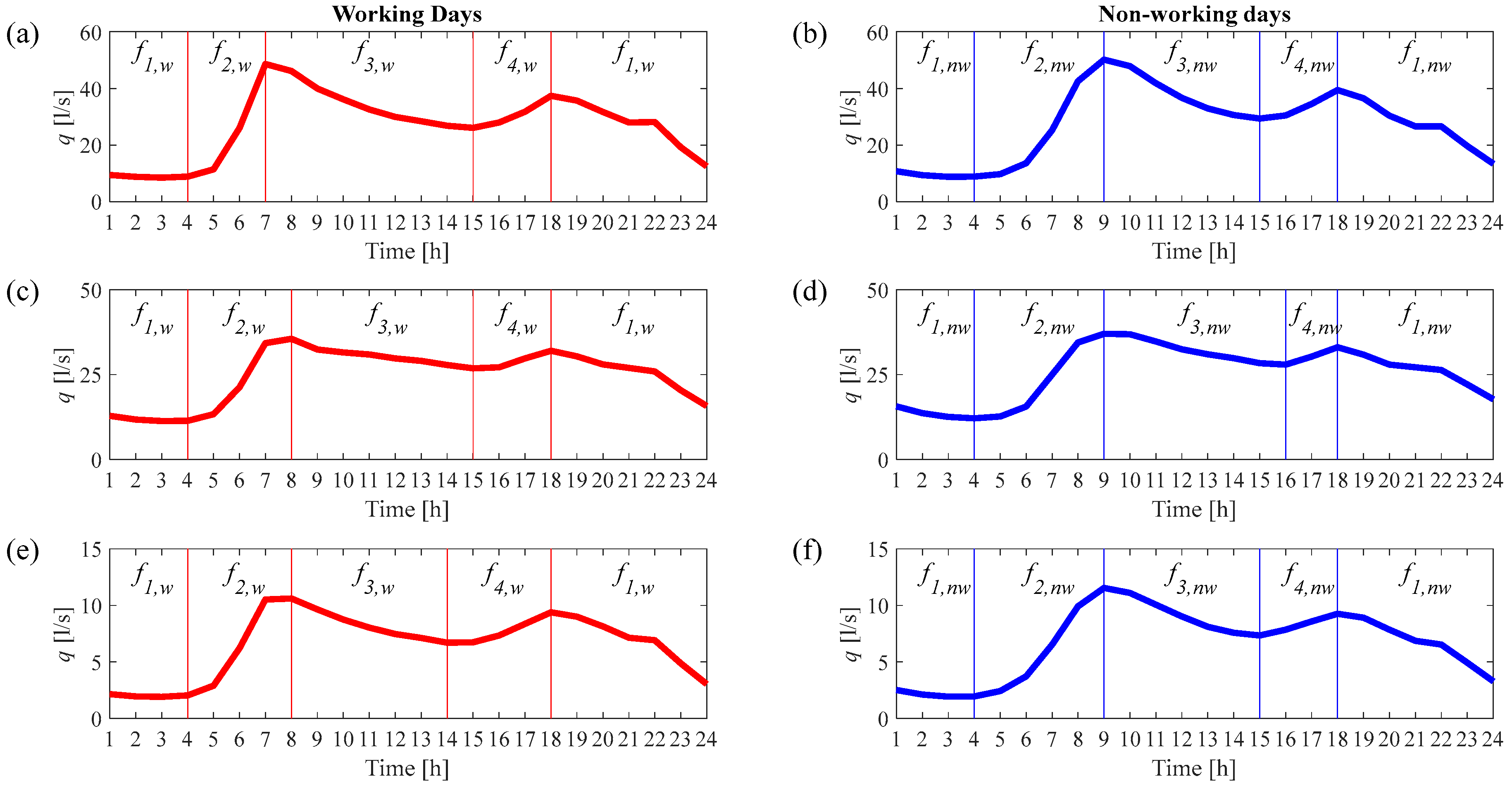
For the purpose of applying the NHMC model, it was necessary to identify the phases into which the generic day can be divided in order to take into account the periodic patterns of hourly demand over the course of the day. Since there was a clear difference between working and non-working days in terms of the hourly water demand patterns, a distinction was made accordingly, which resulted in the identification of different time phases for the two types of days. In particular, these phases, corresponding to the rising and falling phases of demand over the 24 h period, were defined on the basis of the average trend shown by the data relating to the three DMAs, as identified during calibration of the model (see Figure 3).

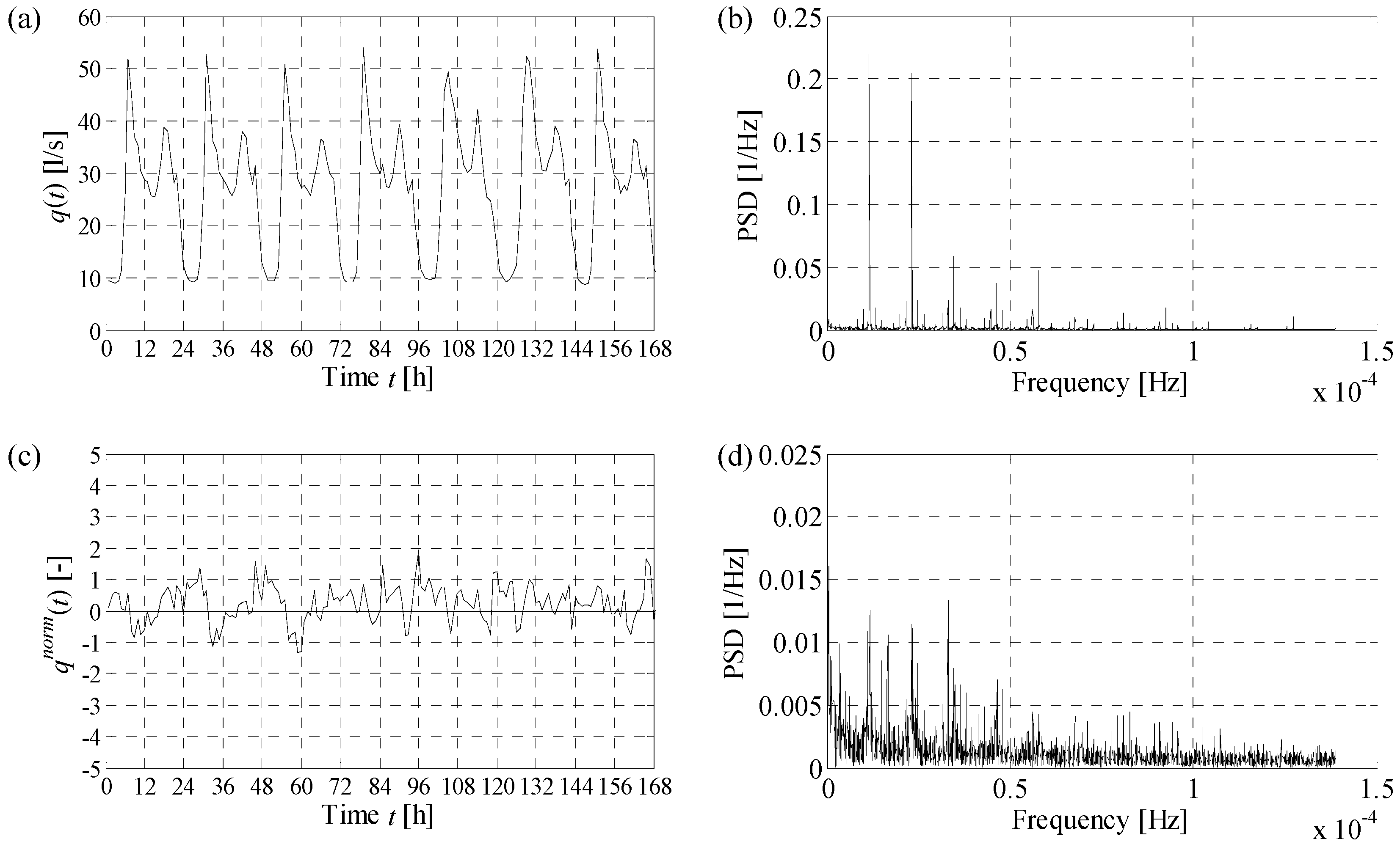
For the purpose of applying the HMC model, data are normalised by using Equation (9). In particular, subtraction at each original water demand q(t) of the mean of the data observed in the calibration phase in the corresponding hour, a distinction being made between working and non-working days, substantially reduces periodicity. This is supported by Figure 4a,c, which show a comparison between observed and normalised hourly demands, respectively, for a one-week period in DMA1. Furthermore, a fast Fourier transform (FFT) algorithm [31] was applied to compute the amplitude of sinusoidal components, as a function of the frequency, characterising the original (Figure 4b) and normalised (Figure 4d) time series. In order to make the results of the analysis comparable, both the time series were preliminary scaled to belong to the [0 1] interval. It can be observed that the original data show strong dominant frequencies at 1.157 × 10⁻⁵ and 2.135 × 10⁻⁵ Hz, corresponding to 24 and 48 h. Even though periodicities are not completely removed by normalisation, the power spectral densities of the normalised series are much more smoothed, and the dominant frequencies at 24 and 48 h are less evident, leading to time series whereto the HMC can effectively be applied, as shown in the subsequent analysis of the numerical results. Similar considerations apply to DMA2 and DMA3.

Two benchmark models were applied by way of comparison to the same datasets, in order to assess the accuracy of the forecasts provided by the NHMC and HMC models. The first benchmark model adopted was a multi-layer perceptron artificial neural network (ANN) model structured in such a way as to provide water demand forecasts for the next K = 24 h. The network has the same structure of the one proposed by Alvisi and Franchini [16], whose inputs are the water demands observed in the past 24 h, normalised in the same manner seen for the HMC model, scaled in the [0 1] interval, and assigned a binary code identifying the type of the day (working or non-working). The second benchmark model used is of the naïve type. The model has a decidedly simpler structure than an artificial neural network, and the specific type used in this study is referred to in the scientific literature as ‘mean’ naïve [32], since it is based on the mean trend in demand during the day. The forecast water demand at each time is assumed to be equal to the mean value of the corresponding hour of the day computed by using the calibration data set.

4. Results and Discussion

The performances of the NHMC and HMC models were first evaluated by considering the deterministic forecasts obtained by these two models (see Equation (5)), and then comparing these with the corresponding forecasts obtained by the ANN and naïve deterministic models. This is followed by the analysis of the additional information provided by the HMC model with regard to the stochastic behaviour of forecasted demands.

For the purpose of evaluating the accuracy of the deterministic forecasts provided by the different models over different time horizons, use was made of the Nash–Sutcliffe index (NS) [33], computed for each forecasting time horizon k comprised between 1 and 24:

$$NS(k)=1-\frac{{\displaystyle \sum _{t=1}^{nd}(q^{obs}(t)-q^{for}(t|t-k\Delta t)}{)}^2}{{\displaystyle \sum _{t=1}^{nd}{(q^{obs}(t)-{\mu }_{q^{obs}})}^2}},$$

(12)

where q^obs(t) is the observed water demands at the time instant t, ${\mu }_{q^{obs}}$ is the mean value of the observed demands, q^for(t|t − kΔt) is the forecasted flow rate kΔt instances before t and, finally, nd is the number of data of the forecasted time series.

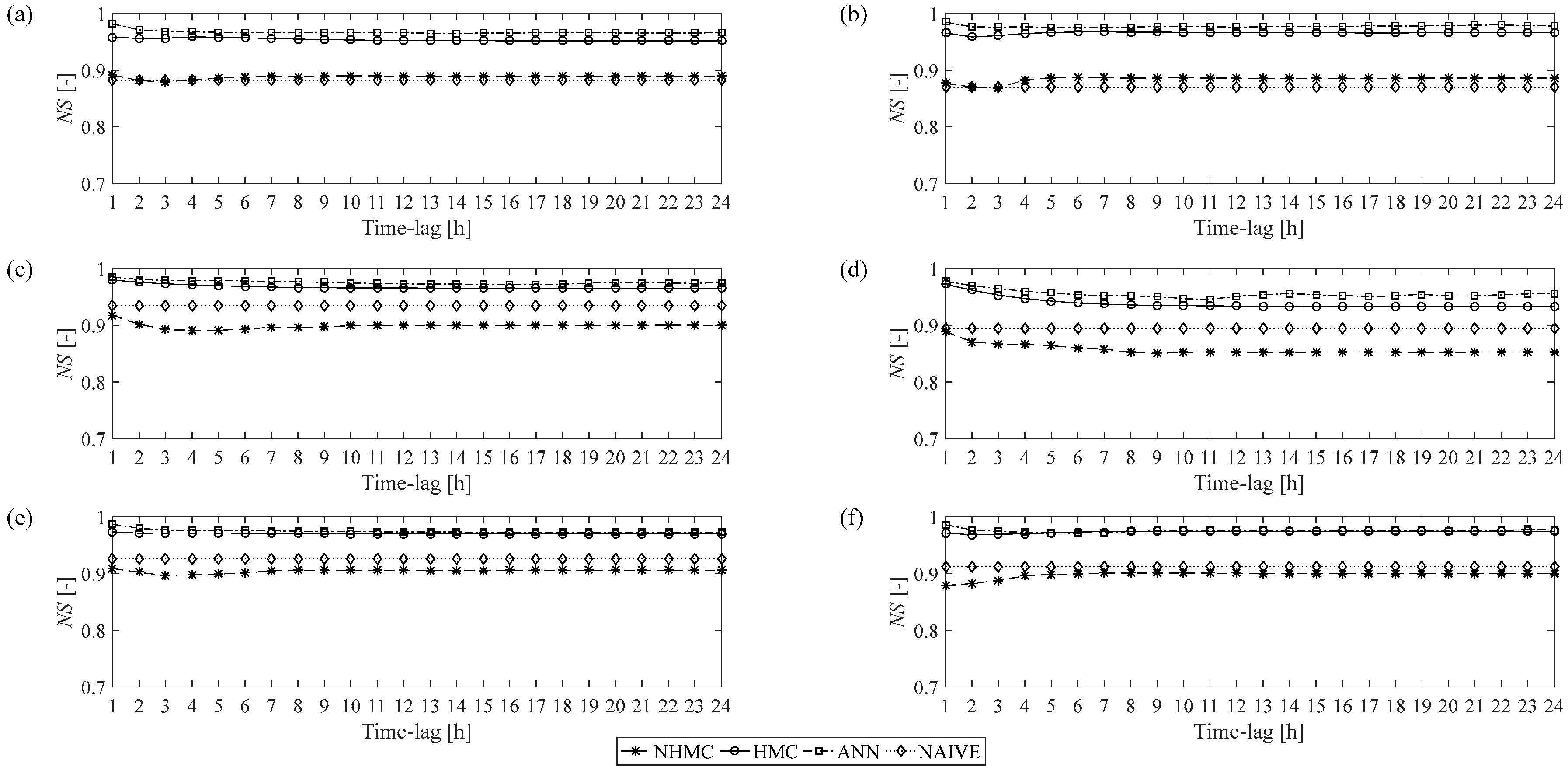
Figure 5 shows the results obtained when the models were applied to the three datasets (i.e., DMAs) during calibration (left-hand column) and validation (right-hand column) phases.

With reference to DMA1, we can observe that in both the calibration (Figure 5a) and validation (Figure 5b) phases, the HMC and ANN models deliver higher predictive accuracy than the NHMC and naïve models. In the calibration phase, the NS indices calculated using the ANN model range from a maximum of 0.98 to a minimum of 0.97, and those calculated using the HMC model between a maximum of 0.96 and a minimum of 0.95. Moreover, both models appear to be stable, since the forecasting accuracy does not undergo appreciable decreases as the time horizon increases. The NHMC and naïve models, by contrast, provide a forecasting accuracy that is very similar, but distinctly worse than that of the HMC and ANN models, with values of NS ranging from 0.89 to 0.88 for NHMC and a value of 0.88 for the naïve model. Similar observations can be made with respect to the results obtained in the validation phase, again for DMA1 (Figure 5b): in the case of the HMC and ANN models, the values of the NS index remained very similar to the ones obtained in the calibration phase, whereas we observe a slight decline in the performance of the NHMC and naïve models. The performance of the models ANN and HMC was substantially the same also in the case of DMA2 and DMA3, as regards both calibration (Figure 5c,e) and validation (Figure 5d,f). For what concerns the NHMC model, it tends to lose effectiveness with respect to the naïve model. It can thus be observed that, insofar as deterministic water demand forecasting is concerned, the HMC model delivers a better predictive accuracy than the NHMC model, and an accuracy that is in line with that of the ANN model. It is worth highlighting that the outperformance of the HMC model with respect to the NHMC can mainly be due to the necessity to estimate several transition matrices for the non-homogeneous model, instead of a single transition matrix, such as for the homogeneous model. In fact, in the HMC model, all the calibration data are used for the estimation of the single transition matrix components, whereas in the NHMC, the calibration dataset is divided into eight sets (see Figure 3), one for each time phase and distinguishing working and non-working days. Thus, a lower number of data is used to calibrate each transition matrix, resulting in a less accurate estimate.

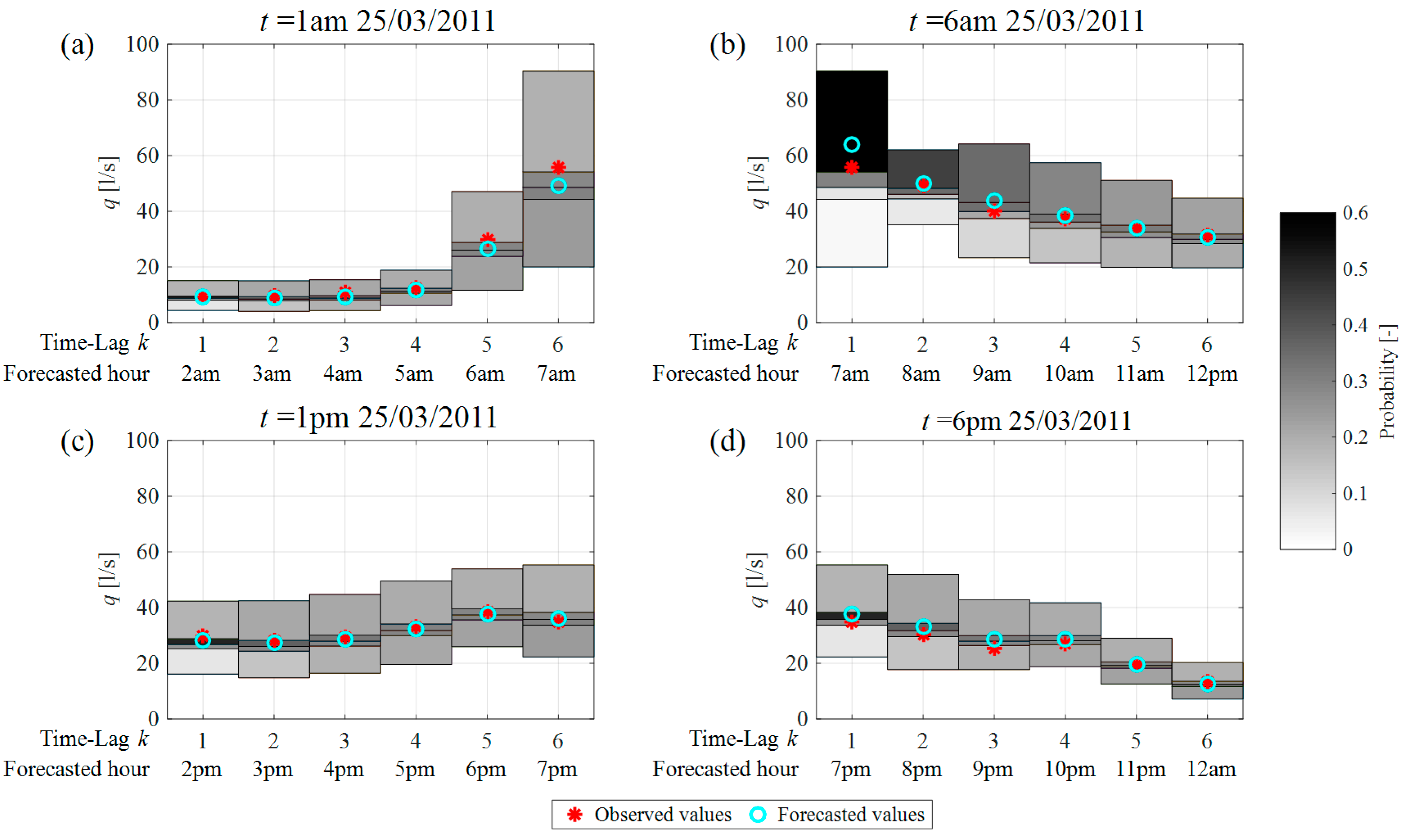
Given above, an analysis on the probabilistic results provided by the HMC model is performed in order to derive some considerations on its prediction capability, as the time horizon varies, to characterise the probability distribution of the water demand at time t + k∆t when forecasted at time t. Figure 6 shows some examples of the results, in probabilistic terms, provided by the HMC model for DMA1. In particular, each graph shows the results provided by the model in relation to the forecasts made at a generic time for the next K = 6 h. The results are here shown with reference to a 6-h forecasting horizon, in order to make the graphs clearer and easier to comprehend and analyse. In fact, each graph contains a representation of the four classes (de-normalised) of water demand values for each of the 6 h of the forecasting time horizon; the background colour of each class, defined on a grey scale as shown in the legend, corresponds to the probability of the future value belonging to that class. The light colours, in particular, represent low probabilities that the future demand will belong to the class, whereas darker colours indicate high probabilities of them belonging to the class. Also shown are the observed and forecasted (deterministically) values for each hour of the time horizon.

For the purpose of interpreting the results, it is important to note first of all that the width of the classes does not depend on the time horizon k considered, but only on the hour of the day to which the forecast refers. In fact, in the case of the HMC model, as previously observed, the classes defined in the normalised space have a width, following de-normalisation, which depends on the standard deviation of the demand in different hours of the day. Let us consider, for example, Figure 6a, which shows the results related to the forecast made at 1 a.m. for the next 6 h, and thus the classes of de-normalised values for the hours between 2 and 7 in the morning. The classes associated with night-time hours (Figure 6a for k = 1,…, 4) have a similar, reduced width, since water demand in these hours shows little variability relative to the mean. The width increases towards the first hours of light and the time the majority of users wake up, and culminates in the peak hour, 7 a.m. (Figure 6a k = 6), where the variability in demand is high. It is further important to observe that the width of the classes in Figure 6a for k = 6, i.e., 7 in the morning, and those in Figure 6b for k = 1 are the same, as Figure 6b refers to the forecast made at 6 a.m. for the next 6 h, and thus k = 1 likewise corresponds to 7 in the morning.

On the other hand, with reference to the Figure 6a, considering the shade of grey in the background of each class, which is proportional to the probability of the future value belonging to that same class, we can observe that for k = 1, the model indicates a high probability that the future water demand will fall in the middle classes 2 and 3 (and the observed data actually does fall in class 2), whereas the probabilities for classes 4 and 1 are much lower (very light grey). As the forecasting time horizon increases, the probability of the future value falling into each of the different classes tends to become uniform (as shown by increasingly similar shades of grey), which is indicative of higher uncertainty in defining the probability to be assigned to each class. This also emerges from a comparison of the probability distributions associated with forecasts of demand at 7 a.m. that are made one hour ahead (Figure 6b k = 1) and 6 h ahead (Figure 6a k = 6). This confirms that the uncertainty in defining the probabilities to be assigned to each class is, as expected, greater when the forecast is made several hours in advance. The same comment applies to other two metering areas, DMA 2 and DMA3.

It is worth remarking that the capability of the MC to define the probabilistic behaviour of future water demand is implicitly contained in its structure and, unlike other existing methods, it requires a minimum computational effort. In other words, due to its own structure, the MC can produce a deterministic forecast and, at the same time, a description of the expected probability distribution of the water demand at time t + k∆t, when the forecast is made at time t. As expected, as the lead time of forecast decreases, the probability estimates become more accurate.

It is also worth noting that we are not presenting, for the MC, uncertainty intervals limited by upper and lower bounds, but instead the entire, even though discretised, probability distribution of the future values as the time of forecast changes. This probability distribution overall characterises the uncertainty, or rather, the variability around the deterministic value forecasted by the model. Unlike the MC method, the ANN model used here, which is based on a standard multi-layer perceptron feedforward ANN, produces only deterministic demand forecasts. This does not mean that it is impossible to produce stochastic forecasts using the ANN—in fact, examples exist in the scientific literature where probabilistic forecasts have been presented e.g., [17,18,20,21,22]. However, this is possible only at the high computational cost due to Monte Carlo simulations typically used in a post-processing phase.

In summary, when compared to ANN-based and similar existing demand forecasting models, the advantage of the MC model presented here, is in its capacity to produce accurate deterministic forecasts and, at the same time, provide additional information on the probabilistic behaviour of future demands, thus characterising their dispersion around the forecasted value, all with minimum computational effort.

5. Conclusions

A new approach to short-term water demand forecasting based on the Markov chain is presented in this paper. The application of a homogeneous and non-homogeneous Markov chain gave rise to two models, which make it possible to estimate the probabilities of future water demand falling within pre-established classes/intervals and, based on these probabilities, provide a deterministic forecast of the future value.

The two models were applied to the water demand time series of three district metering areas, and the deterministic forecasts obtained were compared with the corresponding ones provided by the ANN and naïve forecasting models. The findings showed that the homogeneous Markov chain model (HMC) delivers better forecasting accuracy, matching the prediction accuracy of the ANN model and surpassing the Naïve model one. The homogeneous Markov chain model (HMC) proved to be distinctly more efficient than the non-homogeneous one (NHMC), and is hence preferred to the latter.

The application of the HMC model further demonstrated that probability estimates provided in relation to the state of future demands make it possible to derive, in a computationally efficient manner, useful considerations regarding the probability distribution of the forecasts. Note that this information is not readily available in either of the two benchmark models, and could be obtained only via post-processing analysis, by computationally using much more expensive Monte Carlo simulations. Note also that all this is achieved using a rather simple conceptual structure of the HMC model, which is easy to implement in a suitable software tool. The model also does not need a large amount of data for the calibration of its parameter, since just one transition matrix has to be estimated.

The future work will involve further comparison of the proposed model’s performance to other short-term water demand forecasting models, both deterministic and probabilistic, on several different real life case studies.