Using Probable Maximum Precipitation to Bound the Disaggregation of Rainfall

Abstract

The Multiplicative Discrete Random Cascade (MDRC) class of model is used to temporally disaggregate rainfall volumes through multiplying the volumes by random weights, which is repeated through multiple disaggregation levels. The model development involves the identification of probability density functions from which to sample the weights. The parameters of the probability density functions are known to be dependent on the rainfall volume. This paper characterises the volume dependency over the scarcely observed extreme ranges of rainfall, introducing the concept of volume-bounded MDRC models. Probable maximum precipitation (PMP) estimates are used to define theoretically-based points and asymptotes to which the observation-based estimates of the MDRC model parameters are extrapolated. Alternative models are tested using a case study of rainfall data from Brisbane, Australia covering the period 1908 to 2015. The results show that moving from a baseline model with constant parameters to incorporating the volume dependency of the parameters is essential for acceptable performance in terms of the frequency and magnitude of modelled extremes. As well as providing better estimates of parameters at each disaggregation level, the volume dependency provides an in-built bias correction when moving from one level to the next. A further, relatively small performance gain is obtained by extrapolating the observed dependency to the theoretically-based bounds. The volume dependency of the parameters is found to be reasonably time-scaleable, providing opportunity for advances in the generalisation of MDRC models. Sensitivity analysis shows that the subjectivities and uncertainties in the modelling procedure have mixed effects on the performance. A principal uncertainty, to which the results are sensitive, is the PMP estimate. Therefore, in applications of the bounded approach, the PMP should ideally be described by a probability distribution function.

1. Introduction

Since observed rainfall records tend to be more accurately and completely observed at daily or longer intervals than at sub-daily intervals, temporal disaggregation models are commonly used for the synthesis of sub-daily rainfall as part of flood estimation. Multiplicative discrete random cascades (MDRCs) [1,2,3] make up one class of disaggregation model. Using a MDRC model, the rainfall falling in any interval (say, one day) is divided into two or more sub-intervals (say, two intervals each of 12 h) using a set of weights, W. This is repeated over a number of disaggregation levels until the required time interval (say, one hour) is reached. This requires the probability distribution functions (PDFs) of W to be estimated from rainfall observations. Using the ‘microcanonical’ type of MDRC model, the PDF parameters are estimated for each disaggregation level independently, although empirically derived scaling relationships may be used to generalise between levels.

Much of the work on microcanonical MDRCs has pointed out the strong volume-dependence of the PDF parameters [4,5,6]. This is intuitive; the more rainfall falling in an interval, the more likely the rainfall will be distributed evenly between its sub-intervals, so that the PDF of W is expected to have lower variance around the value W = 0.5. This volume dependence may be included in the model by making the PDF parameters a function of volume [4]; however, due to the low number of observations covering the extreme high rainfall volumes, the PDFs that are most important for flood estimation applications will have high uncertainty. Conversely, obtaining a sufficient number of samples will require a large range of volumes to be used; hence the parameter estimates may not be sufficiently applicable to the relevant extremes. Furthermore, the applicability of the parameter estimates to volumes beyond the observed range yet within the range to be simulated will be unknown. This may contribute to the over-estimation of high rainfall volumes seen in some previous applications of microcanonical MDRC models [5,6,7]. The problem of reducing uncertainty in the parameters of rainfall disaggregation models applicable to high extreme rainfall volumes is the subject of this paper.

The probable maximum precipitation (PMP) is often considered to be an estimate of the theoretical maximum rainfall volume at a given location, time, and space scale. This paper proposes that the PMP can be used to define a theoretical bound on the parameters of the PDFs used for MDRC models. The paper aims to develop this concept into a modelling procedure, test its performance on a case study, and discuss the potential for improvement. While the concept of bounded disaggregation to describe the time scale dependence of parameters, i.e., that the variance of the PDF tends to zero as the time interval becomes shorter, is established [8], the concept of bounding the disaggregation using theoretical volume constraints is new.

2. Theory

The theory presented here is restricted to microcanonical MDRC models in which each interval is divided into two sub-intervals and the disaggregation is symmetrical so that a given volume of rainfall is equally likely to fall in the first sub-interval as in the second. Deeper insight into the theory and application of MDRC models can be found in [7] and the papers cited therein.

The ratio of rainfall volume R (mm) in the time interval t to t + ∆t/2 to rainfall volume in the interval t to t + ∆t is:

$$W= \frac{R_{t:t + ∆t/2}}{R_{t:t + ∆t}}$$

(1)

which we write as

$$W_L= \frac{R_{L+1}}{R_L}$$

(2)

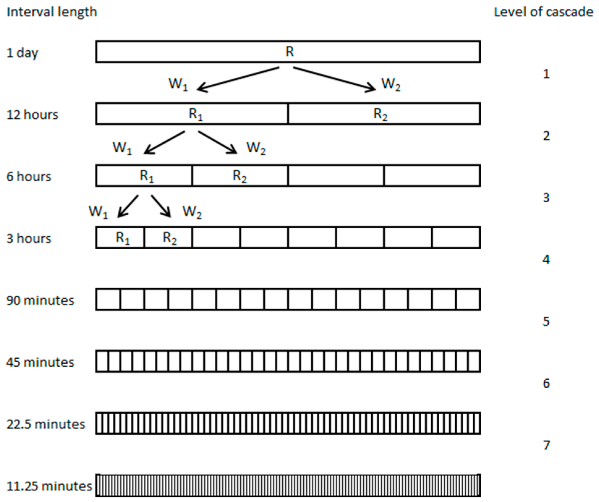
where L is the disaggregation level and N is the total number of levels. For example, Figure 1 shows a cascade with N = 7, where R₁ has a time-step of one day and R₈ has a time-step of 11.25 min. Assuming that volumes are preserved from intervals to sub-intervals, 0 ≤ W_L ≤ 1 and the proportion of the interval’s rainfall falling in the second sub-interval equals 1 − W_L.

A sample of W over each disaggregation level may be obtained from the observed rainfall. The MDRC model may then be estimated by fitting probability distribution functions to the available sample of W. Typically the model has two parts. First, from the probability that W is equal to zero or equal to one, P₀₁, is estimated. Then 1 − P₀₁ is the probability that 0 < W < 1, and, in this range, W is modelled using a probability distribution function, P_x.

The PMP estimate at each level is termed PMP_L. If an available estimate of PMP is taken to be the maximum possible rainfall, then, if the rainfall volume R_L is greater than PMP_L+1, it is impossible for it all to fall within only one of the two sub-intervals, so P₀₁ = 0. More generally, it is impossible for W to be large or small enough for R_L+1 to exceed PMP_L+1. If R_L > PMP_L+1, then:

$$1 - \frac{PM{P}_{L+1}}{R_L} < W_L < \frac{PM{P}_{L+1}}{R_L}$$

(3)

If P_x is assumed to be a uniform distribution, for example [1], for which the only parameters are the upper and lower bounds, deriving P_x from (3) is straightforward. However, in general, alternative distributions are preferable for P_x, in which case the parameters cannot be directly derived from (3).

In the hypothetical case that R_L = 2 × PMP_L+1 because R_L+1 cannot exceed PMP_L+1:

$$W_L=0.5 \mathrm{and}{P}_x={\delta }_{0.5}$$

(4)

where δ_x0 is the Dirac delta. Although hypothetical, (4) provides an asymptote that may be useful for the extrapolation of the observed volume dependency, as illustrated by the case study results.

Henceforth, the subscript L is dropped for convenience of presentation, except where it is necessary to use it because an equation includes variables from two different levels. It should be kept in mind that all model inputs, outputs, and parameters are specific for each level of disaggregation.

3. Methods

3.1. Case Study

Brisbane has an almost continuous 6 min rainfall record from 1908 to 2015. A previous study [6] fitted a number of alternative microcanonical MDRC models to this data set, using 1987 to 2015 for fitting the model and 1908 to 1986 for assessing performance and using the seven levels of disaggregation shown in Figure 1. At each level, they removed the values of W calculated from trace rainfall volumes (R < 0.3 mm) and those calculated from rainfall data with poor quality ratings. They then used the W values calculated using the upper quartile of non-trace R volumes (R ≥ 0.3 mm) to estimate the MDRC model parameters; however, no volume dependency of the parameters was included. The upper quartile was used because the intended application was the simulation of high rainfall. A Beta distribution of W was adopted, and, in the simplest version of the model, symmetry was assumed so that only two parameters, P₀₁ and β, were estimated per level. One of the conclusions was that, while the model performance was considered good, the model tended to over-estimate the high extreme rainfall volumes.

The PMP estimates are derived using the procedures in [9] (22.5 min to 6 h intervals) and in [10] (daily intervals). The PMP for the 12 h interval is linearly interpolated (using units mm/hour) between the 6 h and the daily estimate. The PMP for the 11.25 min interval, which is less than the minimum interval of 15 min used in [9], is estimated by linear extrapolation using 30 min and 15 min estimates. Recognising that there is inherent uncertainty in the procedures for estimating PMP [9,11], the sensitivity of the results to the PMP estimates was tested by replacing the PMP values with Historical Notable Point Rainfall (HNPR) values. These are the historical maxima recorded over Queensland and New South Wales (Brisbane being near the border of these two states) from [12]. Where necessary, the published HNPR values were interpolated to the time intervals used in this study. For the 11.25 min time interval, the interpolated HNPR value (51 mm) was less than the highest value observed in the Brisbane record (75 mm), so the latter was used.

3.2. MDRC Models

Table 1. Method of parameter estimation for different ranges of R for the unbounded baseline and bounded models.

Model		RL ≤ ML	ML < RL ≤ PMPL+1	RL > PMPL+1
Baseline model	P01	Maximum likelihood estimate from the observed [1] W values.
	β	Maximum likelihood estimate from the observed [1] W values (0 < W < 1).
Unbounded model	P01	Logistic regression to describe volume dependency. Estimate parameters using maximum likelihood using all the observed W values.
	β	Maximum likelihood estimate from the observed [1] W values (0 < W < 1).
Bounded model	P01	Logistic regression to describe volume dependency bounded by R = PMPL+1. Estimate parameters using maximum likelihood using all the observed W values.		P01 = 0
	β	Maximum likelihood estimate from the observed [1] W values (0 < W < 1).	Equation (10) to described volume dependency. Parameters of (10) are fixed as described in text.

Note: ^[1] Using only the values of W corresponding to the upper quartile of non-trace R

summarises three MDRC models: the ‘baseline model’, in which the model parameter values are not volume dependent; the ‘unbounded model’, in which the model parameter values are volume dependent but the theoretical bounds provided by the PMP are neglected; and the ‘bounded model’, in which the model parameter values are volume dependent and the theoretical bounds provided by the PMP are included. In all cases, the Beta distribution was used for P_x because it is considered to adequately represent the histograms of observed W values over a broad range of volumes [6].

The baseline model is the two-parameter-per-level model of [6]. Recognising that the model will be applied for high rainfall applications, this model uses the upper quartile of non-trace rainfall observations (i.e., at each level, find all R ≥ 0.3 mm and take the upper quartile of these values) to estimate the parameters.

The unbounded model models the relationship between R and P₀₁ using logistic regression:

$$P_{01}= 1 - \frac{1}{\left(1+e^{-Z_{01}}\right)}$$

(5)

where

$$Z_{01}= a + b{\log }_{10}R$$

(6)

where a and b are the coefficients to be estimated. This permits P₀₁ values to be estimated for any value of R, including those higher than observed during the model fitting period. A comparable log-normal function was used by [4] to model the dependence between R and 1 − P₀₁. For P_x, the values of β used in the baseline model, β_BAS, were maintained because a relationship between R and β was not easily identifiable for all levels from the observed W in the fitting period.

In the bounded model, the same continuous relationship between R and P₀₁ is employed but adjusted so that, from (3), P₀₁ is zero when R equals the PMP of the sub-interval (PMP_L+1).

$$P_{01}=\frac{1}{\left(1+e^{-L_{01}^{\prime }}\right)}-\frac{1}{\left(1+e^{-L_{01}}\right)}$$

(7)

where

$$L_{01}=a+b{\log }_{10}R$$

(8)

$$L{\prime }_{01}=a+b{\log }_{10}PM{P}_{L+1}$$

(9)

For R > PMP_L+1, P₀₁ = 0.

For the bounded model of β, after some trial and error, the following equation was selected:

$${\log }_{10}\beta =c+\frac{1}{{\left({\log }_{10}X-{\log }_{10}R\right)}^d}$$

(10)

where c and d are the coefficients to be estimated and, following (4), X = 2PMP_L+1.

3.3. Parameter Estimation

The parameters a, b, and β_BAS are estimated by maximising the log-likelihood of the model given the fitting period observations of W. An obvious fitting period would be 1987 to 2015 in order to be consistent with the evaluation of the baseline model in [6]. However, that period includes some of the highest extremes in the historical record, and hence evaluating the model on the remaining years would require a limited degree of extrapolation. Instead, therefore, the 12 years in the historical record with the fewest extreme events were identified and used for model fitting. For this purpose, the frequency of extreme events in year Y was defined as N_99Y/N₉₉, where N₉₉ is the number of R values that lie above the 99th percentile of non-trace values, R₉₉, over the entire record and N_99Y is the same number but only counting those values in year Y, scaled according to how many of the missing data lie in that year. N_99Y/N₉₉ was calculated for each of the seven levels of disaggregation and the average taken. The 12 years with the smallest averages were used as the fitting period. In order of an increasing number of extremes these 12 years are 1993, 1908, 1962, 1989, 1913, 1978, 1936, 1911, 1918, 1952, 1944, and 2007.

Estimating parameters c and d in (10) using the observed W is problematic because the fitted model leads to P_x being widely inconsistent with (3). Instead, (3) is used to synthesise a theoretically-based value of β at R = PMP, here called β_PMP, and (10) is required to pass through this value. To estimate β_PMP, a lower bound on W corresponding to R = PMP, here called W_PMP, is identified from (3), and β_PMP is optimised so that the probability of W < W_PMP is equal to an arbitrarily low probability of 0.001. Due to the assumption that P_x is symmetrical, this leads to a 0.002 probability of a W value being sampled from outside the bounds defined by (3) at R = PMP. The baseline model value of β, β_BAS, is maintained up to the maximum observed value of R, M. For R > M, (10) is applied and both c and d are fixed by requiring β to pass through the point [PMP, β_PMP] and also through [M, β_BAS]. The latter means that there is no discontinuity in the volume dependency when moving from R < M to R > M. This approach to estimating P_x therefore has two questionable aspects: the use of β_PMP allows β to be extrapolated to extreme values in a way that is guided by the theoretical bounds defined in (3) but does not strictly honour them; and the value of M is arbitrary rather being estimated from the observations. Why this is a reasonable approach and why alternative models are not useful for the case study will be discussed later in the paper.

3.4. Model Evaluation

All years in the 1908 to 2015 period are used for model performance evaluation. The model output of interest is the high extreme rainfall values, so only the values above R₉₉ are considered in the evaluation. As well as a visual comparison of the histograms of the observed and modelled rainfall, the observed and modelled count of all values above R₉₉ (a metric of frequency of extremes) and the observed and modelled means of all R values above R₉₉ (a metric of magnitude of extremes) are also compared. Achieving a realistic time-structure of rainfall events would require a more complex disaggregation approach, so only the frequencies and magnitudes are evaluated.

Running the model at level L requires that, for each time interval with non-zero R, the first of the two sub-intervals is randomly assigned a zero or non-zero value of W consistent with P₀₁, and any non-zero values of W are then sampled from P_x. The value of R in that sub-interval is then W.R, and the value in the second sub-interval is (1 − W)R.

While the model fitting uses the observed values of W at all levels (Figure 1), most of the results presented below are obtained using only the daily observations of R as inputs. In these cases, for L > 1, the model input for the level L disaggregation is the model output from the level L − 1 disaggregation. This approach is relevant because the intended application of the model is the disaggregation of daily rainfall in periods where sub-daily data do not exist. To gain insight into the origin of errors, the supplementary analysis uses the observed R as the input at each level.

3.5. Sensitivity Analysis

The potentially consequential subjectivities and uncertainties in the development of the models are considered to be those listed in

Table 2. Sensitivity analyses conducted.

Subject of Sensitivity Analysis	Original Setting	Perturbed Setting	Rationale	Mean of All Values > RL99 for 11.25 Mins (mm)	Count of All Values > RL99 for 11.25 Mins
The range of R volumes used to estimate P01 and Px (baseline model, and all models for Px)	Upper quartile of non-trace observed R volumes in fitting period	Upper 2% of non-trace observed R volumes in fitting period	The perturbation may improve the estimate of β applicable to modelling high extreme rainfall	12.9	806
The translation of theoretical bounds on W to values of βPMP (bounded model)	βPMP is set so there is a 0.002 probability of W values being sampled from outside the theoretical bounds	0.02 probability is used instead of 0.002	This will reduce β estimates for R > M, leading to stronger disaggregation and higher extremes	12.7	686
The identification of the point of transition, M, from a constant value of β to volume-dependency (bounded model)	M is the highest value of R observed in the fitting period	M is the highest value of R observed in the entire record	M is unknown and arbitrarily fixed. A higher value of M will reduce β estimates at extremes, leading to stronger disaggregation and higher extremes	13.1	690
The probable maximum precipitation (PMP) estimates (bounded model)	PMP estimates are derived using the Australian standard approaches [9,10]	The Historical Notable Point Rainfall (HNPR) values values are used instead	Although there is no ambiguity about the parameters used to calculate the PMP values, they are generalised across Australia and are high compared to the HNPR values. The latter may be considered a valid empirical rather than theoretical bound	12.8	610
Observed values				11.9	688
Original results of bounded model				12.7	688

. Each of these is subject to a simple perturbation analysis as presented in Table 2.

4. Results

For each of the seven disaggregation levels,

Table 3. Data properties and estimated parameter values.

Level	Time Interval (mins)	PMP (mm)	HNPR (mm)	R99 (mm)	M (mm)		Baseline Model		Unbounded Model		Bounded Model
					Full Period	Fitting Period	P01	log10(β)	a	b	a	b	c	d
1	1440	1440	960	91	311	70	0.40	−0.06	−1.78	2.04	−1.87	2.08	−1.19	0.60
2	720	1242	717	69	228	66	0.29	−0.12	−0.95	1.72	−1.02	1.73	−1.15	0.56
3	360	1043	589	49	167	42	0.29	−0.06	−0.54	1.69	−0.61	1.69	−1.09	0.55
4	180	790	356	36	111	41	0.24	0.00	0.01	1.67	−0.04	1.66	−1.05	0.55
5	90	550	279	26	103	35	0.18	−0.04	0.76	1.65	0.72	1.63	−1.07	0.52
6	45	371	176	18	82	35	0.12	0.04	1.48	2.12	1.46	2.12	−0.99	0.48
7	22.5	250	95	12	82	27	0.05	0.19	2.71	2.34	2.71	2.31	−1.06	0.65
−	11.25	184	75	8	75	18	−	−	−	−	−	−	−	−

shows the model parameter estimates as well as the PMP values and other relevant properties of the data. Two values are given for M; the value for the entire record and the value for the fitting period (in parenthesis). Comparing these two values (and also the R₉₉ values, which are derived from the entire record) indicates the high degree of extrapolation required of the model in its evaluation.

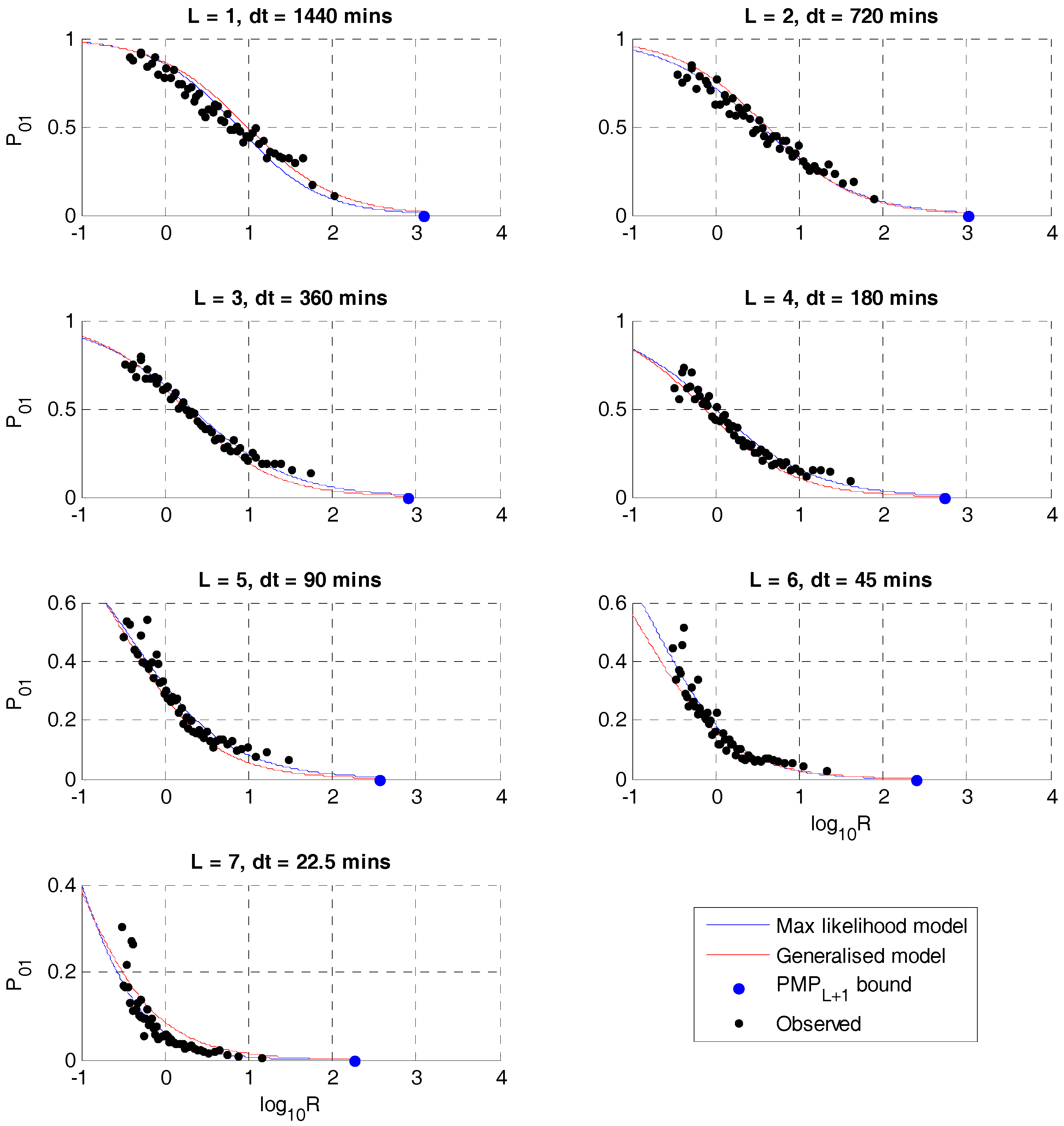
Figure 2 shows the maximum likelihood result for the unbounded logistic regression, (5). Superimposed on this are the ‘observed’ values of P₀₁ estimated by fitting to the observed values of W within each second percentile range of R, plotted against the mean values of R in these ranges, using data from the entire historical record. Although there is considerable noise in these estimates, they show that the logistic regression models are reasonably consistent with the observed volume dependency and that the model identified using only the fitting period translates reasonably to the entire historical record. Also included in Figure 2 are the theoretical point, R_L = PMP_L+1, at and above which P₀₁ = 0 in the bounded model and the results of a generalised model (see Discussion). The results for the bounded model are barely distinguishable from those of the unbounded model so are not included in Figure 2.

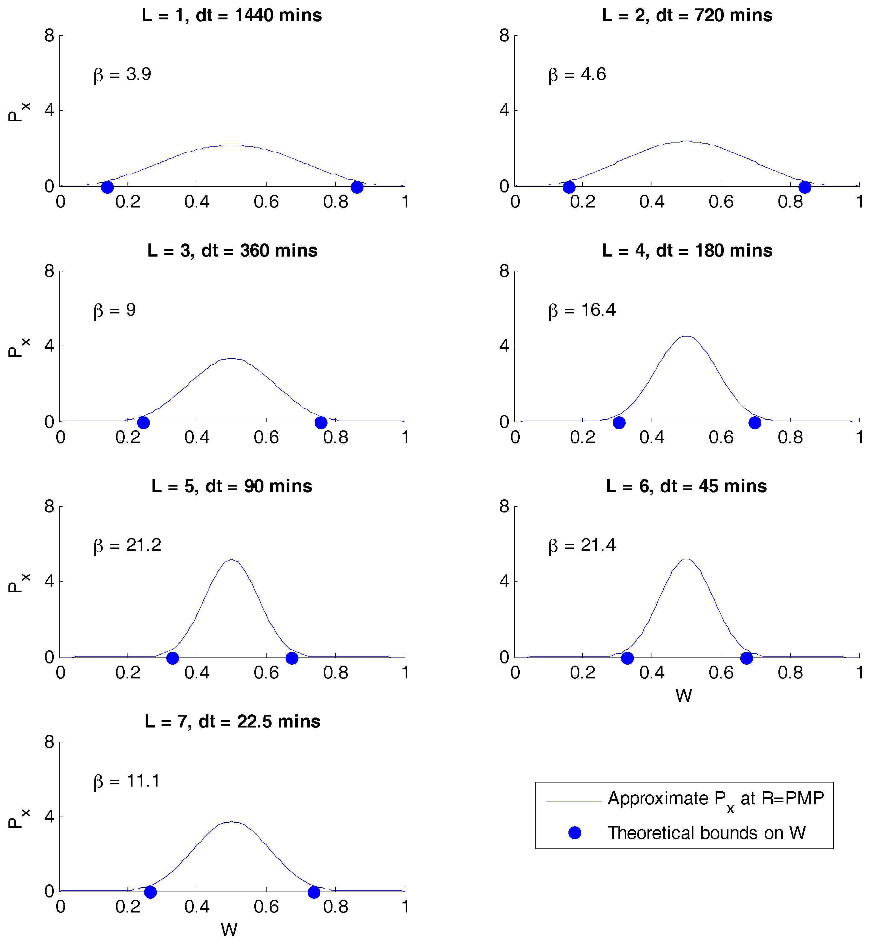
Figure 3 shows the Beta distributions corresponding to the estimate of β_PMP, illustrating the degree to which the theoretical bounds on W are compromised. Figure 4 shows the baseline model estimate of β that is used in all three versions of the model and also the volume dependency of β obtained from (10). Superimposed on these curves are the ‘observed’ values of β estimated using the entire historical record, as previously explained for P₀₁. These ‘observed’ values indicate the errors that arise from using only the fitting period for estimation, most notably at L = 1.

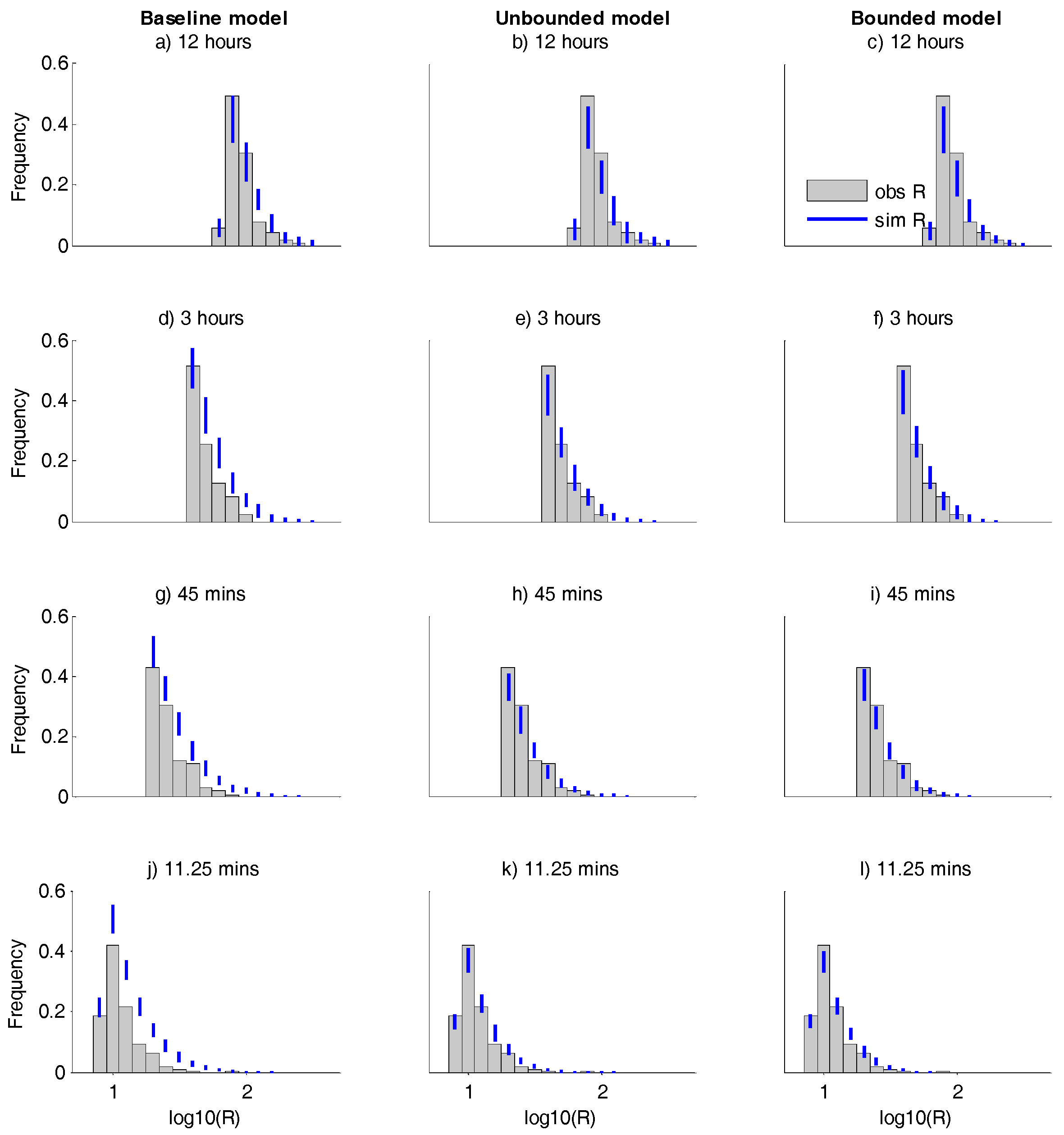
For the same three model baselines, unbounded and bounded, Figure 5 compares the histograms of the observed and simulated extreme rainfall over the 1908–2015 period. The observed and the simulated results in Figure 5 include only the R values that are above R₉₉, and the frequencies are relative to the total number of included observed values. Therefore the differences in the shape and magnitude of the observed and simulated histograms can be used to visually assess the magnitude and frequency performance of the model. For the same set of observed and simulated extremes,

Table 4. Observed and simulated mean R above R₉₉ and the number of R above R₉₉ over 1908–2015.

	Mean R above R99 (mm)				Number of Peaks above R99
	12 h	3 h	45 min	11.25 min	12 h	3 h	45 min	11.25 min
Observed R	93.9	50.1	26.6	11.9	118	215	398	688
Baseline model	103.3 [1]	57.7	31.4	14.8	121 [[2]	283	552	1101
Unbounded model	100.5	54.1	28.4	13.2	103	210	370	710
Bounded model	98.7	51.9	27.1	12.6	100	203	365	688
Bounded model (generalised across levels)	100.6	53.4	27.8	12.9	107	206	342	678
Standard deviation of model results	2.0 [3]	1.1	0.5	0.2	5	10	15	21

Notes: ^[1] This and all subsequent mean values in the table are calculated by: generate 100 realisations of the 1908 to 2015 time-series; for each realization, calculate the mean volume, R_mean, of all modelled R above the observed R₉₉ during 1908 to 2015; calculate the mean of R_mean over the 100 realisations. ^[2] This and all subsequent numbers of peaks in the table are calculated by: generate 100 realisations of the 1908 to 2015 time-series; for each realisation count the number of modelled R values, R_num, above the observed R₉₉ during 1908 to 2015; calculate the mean of R_num over the 100 realisations. ^[3] This and all subsequent standard deviation values in the table are the standard deviations over the 100 samples of R_mean or R_num for the baseline model (the standard deviation values for the other models are within ±5% of this value).

compares the magnitude and frequency metrics. Table 4 also shows the means and standard deviations of the results over the 100 realisations, which, for practical purposes, were the same between models so are only given once.

5. Discussions

This paper explores the concepts of volume bounded temporal rainfall disaggregation. The case study illustrates that using logistic regression to incorporate volume dependency (the unbounded model) can allow more accurate simulation of high extremes than can be achieved using a baseline model that uses constant parameters (Figure 5). Although the volume dependent model tends to over-estimate the magnitudes and under-estimate the frequency (Table 3) of extreme rainfall, this error is small compared to the baseline model error. A further small improvement is obtained by the bounded model, in which the volume dependency is forced to honour theoretically–based bounds derived from PMP estimates.

Although the unbounded and bounded models perform better than the baseline model in general, the results in Figure 5 and Table 4 show that the baseline model is better at predicting the frequency of extreme 12 h rainfall. This may be partly explained by Figure 2, which shows that, at level 1, the logistic regression underestimates the P₀₁ values at log₁₀R > ~1.4, resulting in weaker disaggregation than observed. This error persists even if fitting the logistic regression to the entire record. This may be explained by diurnal convective processes that dominate wet season rainfall in Brisbane, whereby extreme values of daily rainfall are often concentrated in the latter half of the day. In other words, while in general higher volumes mean weaker disaggregation, this is not necessarily the case due to strong convective processes that dominate extremes in this case. As the time–interval decreases, this effect seems to become less important.

The errors at level 1 lead to the recognition that the better overall performance of the unbounded and bounded models is because their level 1 errors are less compounded by level 2 to 7 errors; indeed there is some recovery in performance. The ‘recovery’ is not unexpected as the volume dependence included in these models requires that, if rainfall volumes at level L + 1 tend to be underestimated due to a weak disaggregation at level L, a stronger disaggregation will apply at level L + 1. Therefore, to some extent, the cascade has in–built error correction. Further insight into the role of the level 1 error is gained by removing level 1 and instead making the level 3 to 7 results conditional on the observed 12 h rainfall. This improved performance generally, as it should, except for the number of extremes simulated for the 11.25 min interval, which increased from the original bounded model result of 688 to 733. This further highlights the relevance of how errors compound and cancel over levels, with improved performance at level L not necessarily improving performance at the higher levels. However, when observed R are used as inputs to each disaggregation level, while the performances at levels 2 to 7 were better for all models, the relative performances between models do not change appreciably.

Another point of discussion is whether changes to the baseline model may improve its relative performance. The baseline model is simple, with only two parameters per level, whereas the new unbounded and bounded models both have three parameters estimated from the observations per level. In [6], a number of alternative MDRC models were tested on the same case study using up to 16 parameters per level without including volume dependency. The improvements in extreme value performance using these models are marginal compared with the improvement using the new models. Nevertheless, there may be alternatives to the Beta distribution that lead to more identifiable volume dependencies and improved extreme value performance. For example, differences between the observed and modelled distributions in Figure 5b,c may stem partly from the limitations of the standard Beta distribution [13]. However, using an alternative distribution with more than one parameter would create further challenges for determining the volume dependency.

The results of the sensitivity analysis (Table 2) show that using a more extreme range of rainfall volumes (upper 2nd percentile instead of the original upper quartile) for the estimation of the baseline values of P₀₁ and β deteriorated the performance for all models. This illustrates that restricting the data used for model fitting to a more relevant range of volumes is not useful here due to the lower number of observations and hence higher variance in the baseline estimates of P₀₁ and β. Reducing the PMP estimates to the HNPR values caused the bounded model to substantially underestimate the number of extremes above the threshold R₉₉. This sensitivity confirms that the asymptote defined by (4) is an active constraint and hence that reasonable approximations of PMPs are valuable. Since in practice there is considerable uncertainty in PMP estimates [9,11], applications of the bounded approach to the PMP should ideally be described by a probability distribution function; for example, the approach described by [14] could be adapted. Changing the arbitrary values of β_PMP and M as described in Table 2 also affected the simulated magnitudes and frequencies as expected, although to a relatively small extent.

Several attempts were made to improve upon the bounded model of β. Although this model was considered reasonable, using the standard Beta distribution over all possible values of R allowed the theoretical constraint of (3) to be compromised in the range PMP_L+1 < R_L < PMP_L. An alternative translation of (3), which would avoid this compromise, would be scaling the Beta distribution so that it’s upper and lower bounds are equal to the theoretical bounds calculated from (3). The β parameter could then, in the absence of a better estimate, be fixed at zero (a uniform distribution) or at the baseline model value. An alternative adjustment would be to maintain the standard Beta distribution but to curtail it so that the probability density of W is zero outside the theoretical bounds defined by (3). However, forcing the model to honour (3) is not useful for the case study because a very small number of the observed R are high enough (R_L > PMP_L+1) to be directly affected by (3), and for each of these the probability of an unrealistic sample of W is small. Rather, the value of (3) is supporting the extrapolation of β in the range M_L < R_L < PMP_L+1. Another subjectivity in developing the bounded model of β is the arbitrary value of M, at which the model transitions from the constant baseline value of β to volume dependence. M can be eliminated from the model by applying (10) over the full range of R, in which case c can be fitted to the observations using maximum likelihood and d can be fixed by still requiring (10) to pass through the point [PMP, β_PMP]. This produces a reasonable volume dependency over the higher ranges of R, similar to the results in Figure 4; however it only matches the performance of the original bounded model in the less relevant case that the observed values of R are used as inputs to every disaggregation level.

From the exploration of alternative bounded models of β, it is concluded that the ‘bounded’ concept raises some theoretical challenges due to the facts that (1) P_x must transition, as the PMP value is approached, from a distribution function bounded by the values W = 0 and W = 1 to a distribution function with narrower bounds and (2) sufficient observations of extremes do not exist to examine the transition. Therefore a reasonable judgment of how the theoretical bounds on W should be used to bound P_x as R tends to PMP was necessary in the case study and seems likely to be necessary in future applications. It is possible that pooling extremes from a large number of sites, which adhere to the same volume dependency model, will increase the number of extreme value observations and hence permit a reduced level of subjectivity in developing the model.

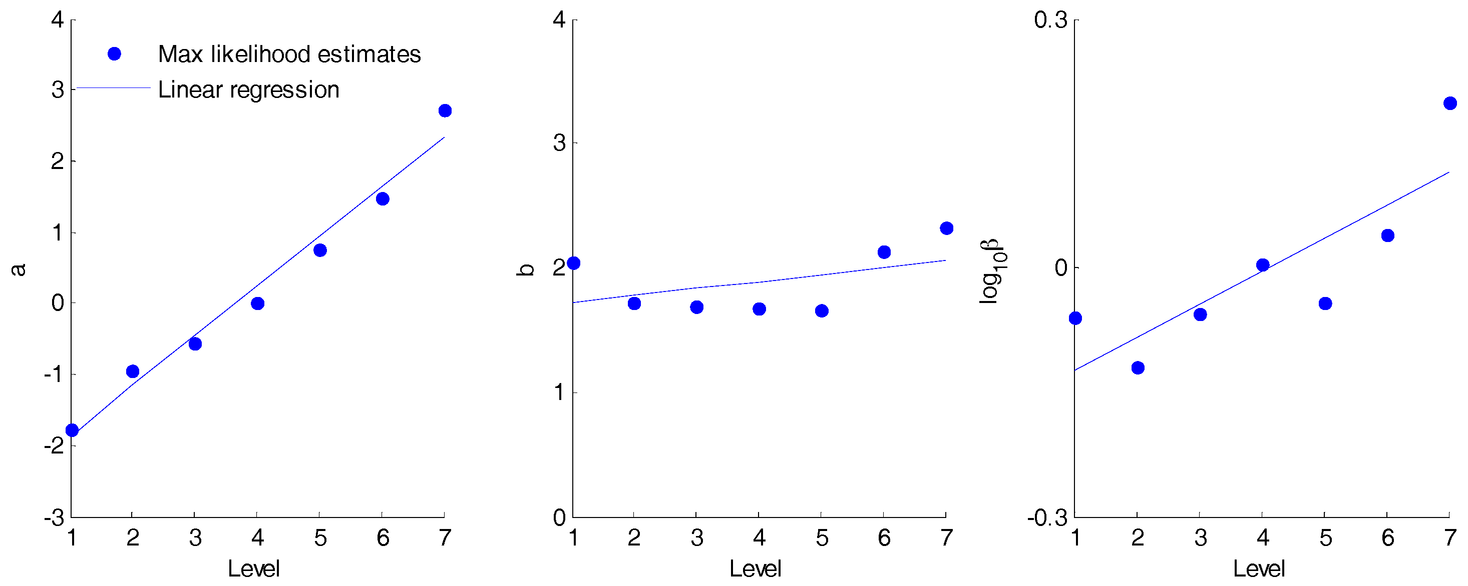
Previous work on this case study [6] found that the baseline model parameters P₀₁ and β can be generalised over the seven disaggregation levels using linear regression. This is potentially advantageous for generating rainfall at unobserved time–resolutions; for example, extrapolating the regression would provide eighth and ninth levels of disaggregation to generate rainfall at approximately 5.6 and 2.8-min intervals. Furthermore, reducing the number of parameters by generalising over levels may assist with the regionalisation of the model. To transfer these potential benefits to the improved, volume–dependent models would require the parameters a and b to be generalised over levels as well as the baseline value of β (recalling that parameters c and d can then be fixed given β_PMP and M). Figure 6 plots the estimates of log₁₀β for the baseline model against L and the estimates of a and b for the bounded model against L. More or less the same results for a and b are obtained for the unbounded model.

From Figure 6, parameter b is taken to be constant and a is taken to be linearly dependent on L (R² = 0.98). There is much less of a relationship between level and log₁₀β than previously found by [6], which must be due to the different fitting periods used (here, the 12 years with fewest extremes; there the 12 available years between 1987 and 2015). It seems that either using a lower range of volumes for fitting the model or relying more on the older pluviograph record rather than more modern tipping bucket data produces less well–behaved β values. To generalise the volume dependency of β, a generalised estimate of the point of transition, M, is also required. For the purpose of illustrating the potential for generalising the model, an arbitrary value, M = PMP/10, is adopted. The generalised volume dependencies are included in Figure 3 and Figure 5. As should be expected, overall, the generalised models are less consistent with the observations than the originals. However, for some levels, the generalisation is actually better, presumably because in these cases the regression smooths out random errors in the original estimates; for example, errors associated with the relatively short fitting period used. The model output statistics for the generalised bounded models, included in Table 4, show a slightly reduced performance compared to the original bounded model but still a considerably better performance than the baseline model. In summary, there is evidence that scaling relationships exist in the bounded and unbounded models, and it is speculated that these are useful for extending the application to unobserved time intervals and regionalisation.

As a final point of discussion, although this paper has focused entirely on the MDRC type of model, the principle that rainfall disaggregation can be bounded by the consideration of PMPs could be applied more broadly. This may include, in the context of climate change impacts on rainfall, deriving the volume-dependence of change factors and their PMP-derived bounds in much the same way as Figure 4 has been constructed, noting that the consideration of climate change may require the PMPs to be treated as non-stationary.

6. Conclusions

The concept of bounding the volume dependence of rainfall disaggregation model parameters using PMP estimates has been formally developed. Applying a MDRC model to the simulation of short-duration, point-scale rainfall at a site in Brisbane, the new approach is seen to be capable of improving simulations of extreme rainfall. However, the main improvement on the constant-parameter baseline model comes from including a reasonable volume dependency without the PMP-based bounds. This is associated with obtaining improved estimates of the model parameters for the rarely observed extreme volume ranges and the ability of the cascade to self-compensate for errors. An initial exploration shows that the volume dependencies are scalable across time resolutions, showing promise for an extended range of applications. The method should be tested on other gauges that represent a broader range of extreme rainfall distributions

References

1. Olsson, J. Evaluation of a cascade model for temporal rainfall disaggregation. Hydrol. Earth Syst. Sci. 1998, 2, 19–30. [Google Scholar] [CrossRef]
2. Deidda, R.; Benzi, R.; Siccardi, F. Multifractal modeling of anomalous scaling laws in rainfall. Water Resour. Res. 1999, 35, 1853–1867. [Google Scholar] [CrossRef]
3. Onof, C.; Townend, J.; Kee, R. Comparison of two hourly to 5-min rainfall disaggregators. Atmos. Res. 2005, 77, 176–187. [Google Scholar] [CrossRef]
4. Rupp, D.E.; Keim, R.F.; Ossiander, M.; Brugnach, M.; Selker, J.S. Time scale and intensity dependency in multiplicative cascades for temporal rainfall disaggregation. Water Resour. Res. 2009, 45. [Google Scholar] [CrossRef]
5. Pui, A.; Sharma, A.; Mehrotra, R.; Sivakumar, B.; Jeremiah, E. A comparison of alternatives for daily to sub–daily rainfall disaggregation. J. Hydrol. 2012, 470–471, 138–157. [Google Scholar] [CrossRef]
6. McIntyre, N.; Shi, M.; Onof, C. Incorporating parameter dependencies into temporal downscaling of extreme rainfall using a random cascade approach. J. Hydrol. 2016, 542, 896–912. [Google Scholar] [CrossRef]
7. Molnar, P.; Burlando, P. Preservation of rainfall properties in stochastic disaggregation by a simple random cascade model. Atmos. Res. 2005, 77, 137–151. [Google Scholar] [CrossRef]
8. Menabde, M.; Sivapalan, M. Modeling of rainfall time series and extremes using bounded random cascades and Levy–stable distributions. Water Resour. Res. 2000, 36, 3293–3300. [Google Scholar] [CrossRef]
9. Bureau of Meteorology. The Estimation of Probable Maximum Precipitation in Australia: Generalised Short–Duration Method; Bureau of Meteorology: Melbourne, Australia, 2003; p. 39. [Google Scholar]
10. Bureau of Meteorology. Guidebook of the Estimation of Probable Maximum Precipitation: Generalised Tropical Storm Method, Included on Compact disc ‘Guide to the Estimation of Probable Maximum Precipitation: Generalised Tropical Storm Method’, Hydrometeorological Advisory Service; Bureau of Meteorology: Melbourne, Australia, 2004. [Google Scholar]
11. Micovic, Z.; Schaefer, M.G.; Taylor, G.H. Uncertainty analysis for Probable Maximum Precipitation estimates. J. Hydrol. 2015, 521, 360–373. [Google Scholar] [CrossRef]
12. Bureau of Meteorology. Australia’s Record Rainfall. Available online: http://www.bom.gov.au/water/designRainfalls/rainfallEvents/ausRecordRainfall.shtml (accessed on 22 February 2017).
13. Licznar, P.; De Michele, C.; Adamowski, W. Precipitation variability within an urban monitoring network via microcanonical cascade generators. Hydrol. Earth Syst. Sci. 2015, 19, 485–506. [Google Scholar] [CrossRef]
14. Fernandes, W.; Naghettini, M.; Loschi, R. A Bayesian approach for estimating extreme flood probabilities with upper–bounded distribution functions. Stoch. Environ. Res. Risk Assess. 2010, 24, 1127–1143. [Google Scholar] [CrossRef]
Figure 1. Schematic of the employed Multiplicative Discrete Random Cascade (MDRC), wherein daily data are disaggregated into 11.25 min data using seven cascade levels (from [6]; adapted from [1]).
Water 09 00496 g001
Figure 2. Volume dependence of P01 for the unbounded model.
Water 09 00496 g002
Figure 3. Beta distribution functions used to represent the theoretical bounds on W at R = PMP.
Water 09 00496 g003
Figure 4. Volume dependence of parameter β.
Water 09 00496 g004
Figure 5. Comparison of observed and simulated extreme rainfall using the baseline, unbounded and bounded models.
Water 09 00496 g005
Figure 6. Generalised models of parameters a, b, and log10β for the bounded model.
Water 09 00496 g006