Better-Fitted Probability of Hydraulic Conductivity for a Silty Clay Site and Its Effects on Solute Transport

Abstract

The heterogeneous hydraulic conductivity of a subsurface medium is vital to the groundwater flow and solute transport. Probability is efficient for characterizing and quantifying the field characterization of hydraulic conductivity. Compared with sandy mediums, silty clay is paid less attention to due to its low hydraulic conductivity. For long-term solute transport and seawater intrusion, the low-permeable medium is considered as a remarkably permeable medium. This study reports on a comprehensive investigation on the hydraulic conductivity field of the Ningchegu site, located east of Tianjin City of China. Four layers recognized by 52 boreholes, plain fill, continental silty clay, mud–silt clay and marine silty clay, were deposited from the top to the bottom. The hydraulic conductivities measured via permeameter tests ranged from 2 × 10⁻⁶ m/d to 1.6 × 10⁻¹ m/d, which corresponded to the lithology of silty clay. The magnitude and the range of the hydraulic conductivity increased with the depth. Five probability distribution models were tested with the experimental probability, indicating that a Levy stable distribution was more matched than the log-normal, normal, Weibull or gamma distributions. A simple analytical model and a Monte Carlo technique were used to inspect the effect of the silty clay hydraulic conductivity field on the statistical behavior of the solute transport. The Levy stable distribution likely generates higher peak concentrations and lower peak times compared with the widely-used log-normal distribution. This consequently guides us in describing the transport of contaminations in subsurface mediums.

1. Introduction

The emphasis on hydraulic conductivity (K) is contributed by Darcy’s law, and the field-measured values of K are of well-known heterogeneity with over 13 orders of magnitude [1]. Groundwater contamination has become one of the most important environmental issues all over the world. It is necessary to predict groundwater flow and solute transport in order to protect groundwater quality. However, the heterogeneity of porous media and the incomplete knowledge of data information lead to difficulties in the estimation of hydraulic properties and geophysical variables, and thus create difficulty in estimating or predicting the subsurface flow and transport.

The representation of hydraulic conductivity distributions is an important issue in predicting the groundwater flow field [2] and subsurface contaminant transport [3]. Several equations of the contaminant transport make assumptions regarding the properties of hydraulic conductivity, including the probability density function (PDF) [4]. The hydraulic conductivity of aquifer materials has most often been found to be log-normally distributed [5,6,7,8,9,10,11]. Sanchez-Vila et al. [12] demonstrated numerically that randomly varying transmissivities could exhibit a scale effect because of deviations from the log-normal distribution. Hyun [13] reported that the log permeability data at the Apache Leap Research Site (ALRS) near Superior, Arizona, were indeed represented more accurately by a Levy stable distribution than by a Gaussian distribution, and inferred that the permeability scale effect was probably true at many other sites.

The lithologies of aquifer mediums from MADE (Macro-Dispersion Experiment test site) [14], Borden [9], and Cape Code [7], regarded as the three most popular hydrogeological test sites, are generally sand, gravel, and sandy material mixed with lenses of silt. Vereecken and Doring [15] investigated the spatial variability of basic aquifer parameters and hydraulic conductivities using data from the clay and silt from Krauthausen experiment.

Most of the studies on the effect of heterogeneous hydraulic conductivity on solute transport were focused on the heterogeneous aquifer. However, PDFs of low K and the effect on flow and solute transport were not reported through literature. This could have resulted from testing difficulties in terms of low-K mediums with weak migration and solute abilities [11,16].

Stochastic methods were developed and used to deal with these difficulties [17].The stochastic simulation technique was applied to quantitatively study the impact of hydraulic conductivity heterogeneity on groundwater solute transport [18]. The study by Kohlbecker et al. [2] indicated that Levy stable distributions with increments in the log conductivity gave rise to Levy stable distributions with increments in the logarithm of the velocity (ln u) using Monte Carlo and MODFLOW (U.S. Geological Survey modular finite-difference flow model) techniques. Wang and Huang [3] analyzed the impact of hydraulic conductivity on solute transport processes in a highly heterogeneous aquifer. Few analyses were reported on the characteristic parameters of solute transport using stochastic test methods.

The twofold objectives of this study were to investigate the probability distribution of a low K, and the effects of PDFs on solute transport according to the collected data. The field study for the sampling and permeameter tests performed at the Ningchegu (NCG) site are introduced first. Then the statistics of a low-K field are shown, especially the statistical distributions of the low-K data tested by five widely used distributions. Finally, the effects of PDFs on solute transport were analyzed using a simple analytical model. The effects of Levy stable distributions on solute transport were compared with log-normal distributions.

2. Materials and Methods

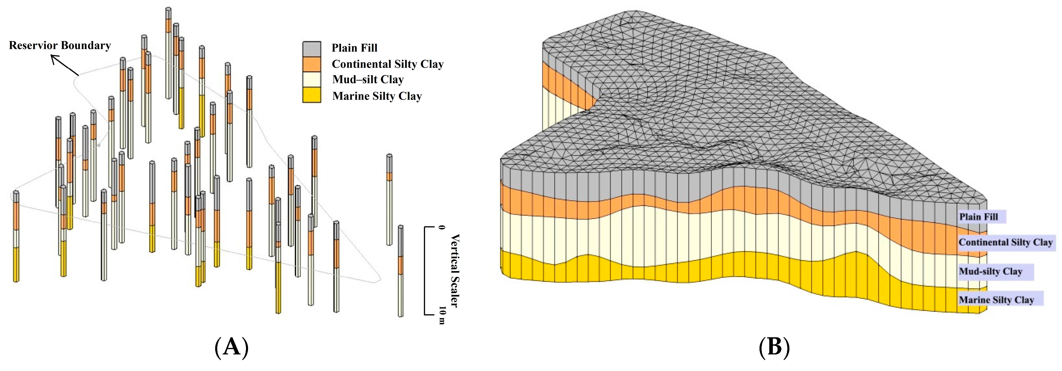
2.1. Sampling and Lithology

The locations of boreholes are within the eastern Tianjin city, around 5 km west of the Bo Sea. This area was considered as a candidate of the NCG reservoir, resulting in the collection from dozens of boreholes during August to November of 2011 to depict the lithology at different depths. In total, 52 boreholes (Figure 1A) were evenly installed around an area of 6.2 km² at an areal density of 8 boreholes/km². The average distance of each pair of two boreholes was 345 m. Each borehole was drilled up to a depth of 10 m, and different samples (3~5 cores per borehole) were collected according to the diversity of the lithology. The cylinder sampler used was 20 cm in length and 110 mm in inner diameter. The undisturbed samples were then moved to a laboratory at Hohai University to test their hydraulic conductivities. In terms of the lithology of sediments in the study area dominated by clay and silty clay, a recommended falling head method [1] applied to the fine material was used to analyze the hydraulic conductivity of the core using a permeameter (TST-55; Φ: 61.8 mm × 40 mm; made in China). The infiltration process for low-K sediments was quite slow, and a successful permeameter test averagely took more than 6 hours in our study. Therefore, eight permeameters were used to test different clay samples, simultaneously. In total, we finished 212 falling head permeameter tests to investigate the hydraulic conductivity of the reservoir sediments.

A thick, loose Quaternary sediment layer, which is a continental-dominated paralic deposition, covers the eastern area of Tianjin city. The lithology is mainly composed of clay, silty clay, and sand lens, formed from alluvium of the Hai River and Ji Canal [19]. Based on the information collected from borehole drilling, a 3-D lithology model was developed (Figure 1B). Four layers were identified by drilling, including the shallowest layer of plain fill with a thickness of between 1 and 1.5 m. The second shallowest layer of continental silty clay had a thickness of 0 to 3.4 m, indicating that some areas lacked the material of continental silty clay. The third mud–silt clay layer was buried below the second layer, with of thickness of 0 to 7.0 m, and the deepest layer of marine silty clay had a thickness of 0 to 7.3 m. Based on the borehole information, the study area was completely covered with the plain fill, but the other three layers somewhat showed stratum absence. The fourth layer of marine silty clay was only revealed at down to, but not limited to, 10 m of the boreholes, and the lack of the fourth layer locally came from the limited drilling depth of 10 m. The first and second layers were noticeably thinner than the two deeper layers shown in Figure 1B.

2.2. Method of Statistics

The statistical values of hydraulic conductivities from each layer were summarized, including the minimum (min), maximum (max), mean (mean), and standard deviation (SD). Furthermore, finding the probability distribution of hydraulic conductivities for each layer was one key objective of this study, and these were tentatively fitted by the two mostly widely used probability distributions (Gaussian and log-normal distributions), and Levy stable, gamma and Weibull distributions.

The Gaussian distribution is one of the most commonly used statistical models. A Gaussian distribution is associated with a bell shape, with very large/small values appearing in a low probability. However, strongly heterogeneous fields are not uncommon in nature, and very large/small properties may appear frequently in such geologic formations. A log-normal distribution is a continuous probability distribution of a random variable whose logarithm is normally distributed, which is widely used in geophysical variables. The logarithmic transform is a common means to seek a more appropriate distribution for a random variable [20]. $\mu$ and $\sigma$ are the mean and standard deviation of the Gaussian or log-normal distributions, respectively.

To describe the statistical characteristics of heterogeneous fields, a Levy stable distribution has recently been proposed to analyze geological data [2,21,22]. Except for very few cases such as the Gaussian (normal) and Cauchy distributions, the closed-form expressions for density and distribution functions of the Levy stable distribution are not available [23].The characteristic function most often employed in numerical calculations is the following [24]:

$${\phi }_0(t)=\{\begin{array}{ll}\exp \left(-{\gamma }^{\alpha }{\left|t\right|}^{\alpha }\left[1+i\beta (\tan \frac{\pi \alpha }{2})(signt)({\left|\gamma t\right|}^{1-\alpha }-1)\right]+i\delta t\right),& \alpha \ne 1\\ \exp \left(-\gamma \left|t\right|\left[1+i\beta \frac{\pi }{2}(signt)(\ln \left|t\right|+\ln \gamma )\right]+i\delta t\right),& \alpha =1\end{array}$$

(1)

where ${\phi }_0$ is the characteristic function; $\alpha$ is a Levy index with a range of 0–2; $\beta$ is a skewness parameter ranging between −1 and 1; $\gamma$ is a scale parameter in the interval (0, +∞), corresponding to the standard deviation of the Gaussian distribution; $\delta$ is a shift parameter; i is the imaginary part of a complex number; and sign(t) is a logical function that extracts the sign of a real number t. A symmetric Levy stable distribution with a zero mean is determined when β = 0. A standard Levy stable distribution has γ = 1 and δ = 0.

In addition, the gamma and Weibull distributions, which are also popular asymmetric and heavy-tailed distributions, were used to test the probability distribution of the silty clay hydraulic conductivity. The PDFs of the gamma and Weibull distributions are as follows. The PDF of the gamma distribution is

$$f(x)=\frac{1}{b^a\mathrm{\Gamma }(a)}{x}^{a-1}{e}^{-\left(\raisebox{1ex}{$x$}\!\left/ \!\raisebox{-1ex}{$b$}\right.\right)}$$

(2)

where $\mathrm{\Gamma }(\cdot )$ is the gamma function.

The Weibull PDF is positive only for positive values of x, and is zero otherwise. For strictly positive values of the shape parameter b and scale parameter a, the density is

$$f(x)=\frac{b}{a}{\left(\frac{x}{a}\right)}^{b-1}{e}^{-{\left(\raisebox{1ex}{$x$}\!\left/ \!\raisebox{-1ex}{$a$}\right.\right)}^b}$$

(3)

Both the Weibull distribution and the gamma distribution can give exponential distributions with particular choices of one of their two parameters. The PDF curves of the Weibull and gamma distributions are more complex compared to those of a standard exponential distribution, mainly because both of the two distributions have two independent parameters.

The primary means to test whether the data follow a specific distribution is by using nonparametric test procedures [25]. Taking the normal distribution as an example, the null hypothesis (H0) for all tests of normality is that the data are normally distributed. Rejection of H0 says that this is doubtful. Failure to reject H0, however, does not prove that the data do follow a normal distribution, especially for small sample sizes. It simply says that normality cannot be rejected with the evidence at hand. The Kolmogorov–Smirnov (K–S) test is widely used to serve as a goodness of fit test [26]. Moreover, the Anderson–Darling (A–D) test is a statistical test for whether a given sample of data is drawn from a given probability distribution [27]. Therefore, these two nonparametric tests were applied to test the similarity with the given probability distributions.

2.3. Random Modeling of Solute Transport to K Distribution

The migration of pollutants satisfies the convection–diffusion equation in a saturated medium. The 1-D steady flow dynamic dispersion model is a relatively simple and widely used method in the convection–diffusion problem. Particularly, in a 1-D infinite column filled with a porous medium, under the condition of an instantaneously injected tracer, the analytical solution of the solute concentration in the medium is described as the following [28]:

$$C(x,t)=\frac{m/w}{2n_e\sqrt{\pi D_{L}t}}{e}^{-\frac{{(x-ut)}^2}{4D_{L}t}}$$

(4)

where x is distance from the injection point in meters, t is time (d), C(x,t) is the tracer concentration (g/L), m is the tracer mass (kg), w is the cross-sectional area (m²), u is the flow velocity (m/d), n_e is the effective porosity, and D_L is the longitudinal dispersion coefficient (m²/d).

The time is labeled as the peak time (t_p) when the solute reaches the maximum concentration at a distance from the injection point, and the corresponding concentration is called the peak concentration (C_p). The migration distance x is set when the first derivative equals zero (dC/dt = 0); the peak time (t_p) is written as the following:

$$t_p=\frac{-D_L+\sqrt{D_L^2+x^2{u}^2}}{u^2}$$

(5)

The peak concentration (C_p) is acquired via the peak time (t_p):

$$C_p=\frac{m/w}{2n_e\sqrt{\pi D_L{t}_p}}{e}^{-\frac{{(x-u{t}_p)}^2}{4D_L{t}_p}}$$

(6)

The peak time and the peak concentration are two important characteristics used to describe the process of solute transport in a saturated–unsaturated medium. Based on this method, the maximum negative effects and emergency time of the solute (pollutants) can be recognized, to some extent. It is noted that these simple analytic equations were concluded in the conditions of a 1-D infinite domain and instantaneously injected pollutants, which is actually a homogeneous rather than heterogeneous domain. However, in water-environment-related issues, the governor or institution needs to make decisions quickly and accurately, and most of the decisions come from technical support using these simple solutions. Due to the uncertainty of probability distributions of K, the offset of induced outcomes will be addressed herein.

While the PDF cannot always be explicitly expressed, such as for the Levy stable distribution, the Monte Carlo method [29] is an alternative method, compared with inverse function methods, to simulate the random characteristics of pollutants’ transport. According to the statistical characteristics of K, combined with the data from the NCG site, the Monte Carlo technique was used to produce random hydraulic fields, to further inspect the effect of random distributions of K on t_p and C_p. In terms of unclosed forms of the Levy stable distribution, the CMS (Chambers-Mallows-Stuck) method involved in a MATLAB toolbox developed by Liang and Chen [23] was applied herein to generate the Levy random number.

This study will focus on analyzing the applicability of the Levy stable distribution for describing heterogeneity characteristics of a low K in this test site. In addition, it is common to apply the log-normal distribution for numerical simulations [30]. In order to further compare the solute transport of two distributions in saturated mediums, a large number (10,000) of the hydraulic conductivity values following the corresponding distribution were produced using the Monte Carlo method, and combined with the actual regional hydrostratigraphic situation to eliminate negative and maximum values (a value of K larger than 0.6 m/d was not considered as a low permeability medium).

3. Results and Discussion

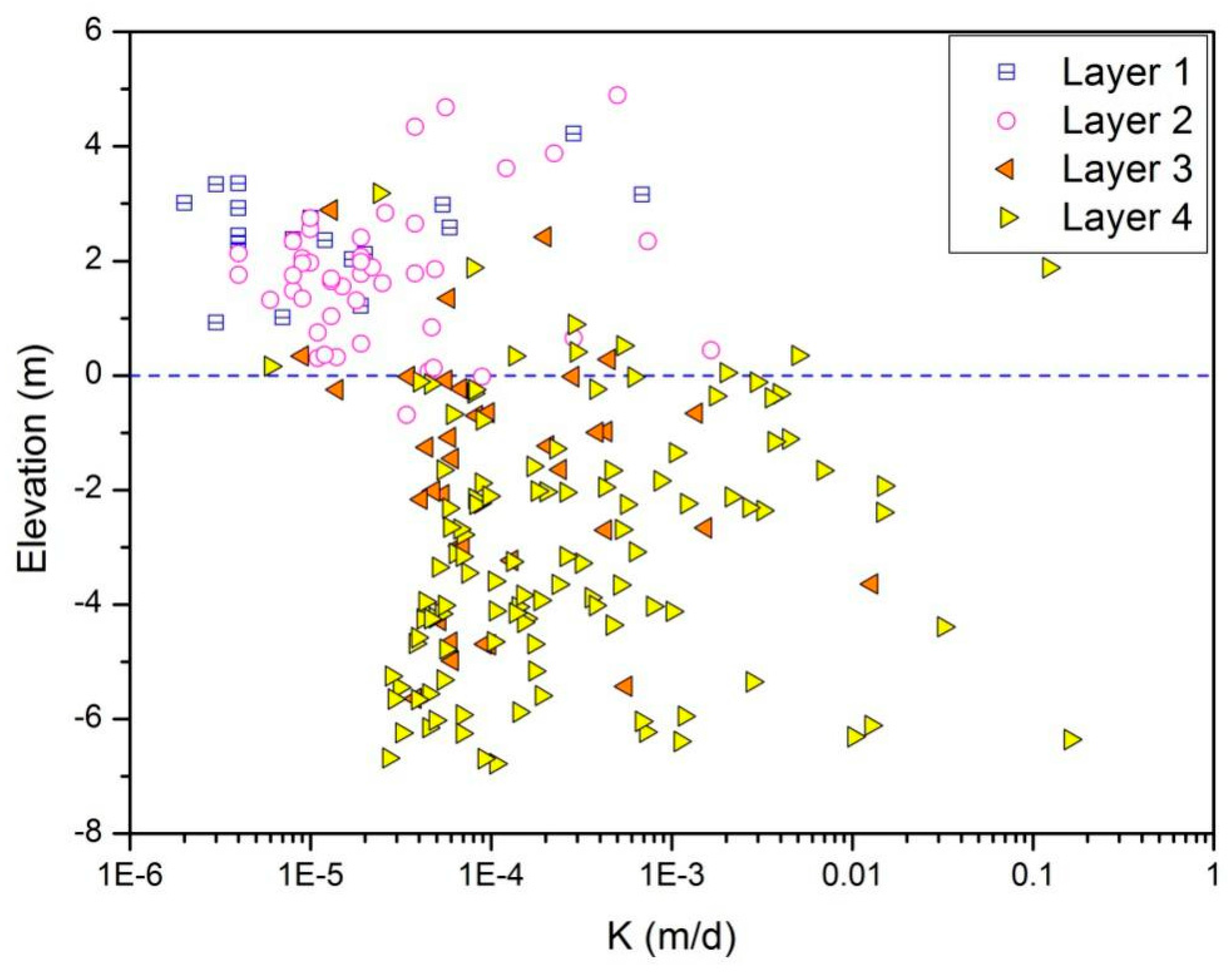
3.1. Hydraulic Conductivity of the Silty Clay Medium

The K values were analyzed according to their identical lithologies, and the general statistics of K values from each layer are listed in

Table 1. Tested hydraulic conductivity and the lithology of the NCG site.

Geologic Material		First Layer	Second Layer	Third Layer	Fourth Layer
K (m/d)	Min	2 × 10−6	4 × 10−6	9 × 10−6	6 × 10−6
	Max	6.8 × 10−4	1.6 × 10−3	1.3 × 10−2	1.6 × 10−1
	Mean	6.7 × 10−5	9.5 × 10−5	5.6 × 10−4	3.9 × 10−3
	SD	1.68 × 10−4	2.79 × 10−4	2.12 × 10−3	1.92 × 10−2
Sample size		18	46	36	112
Lithology		Plain fill	Continental silty clay	Mud–silt clay	Marine silty clay

. Figure 1B also illustrates that the different types of geologic sedimentary processes gave rise to different types of stratigraphy facies. The sediments of each layer, from the shallow to the deep respectively, were plain fill, continental silty clay, mud–silt clay and marine silty clay. Given the very different physical/chemical origins of different facies, it likely did not make sense to conduct statistical analyses based on combined data from multiple facies.

The sample sizes of the deepest and the shallowest layers were 112 and 18 respectively, representing the largest and smallest sizes in the four layers. The minimum K values of the four layers had insignificant differences within the same order of magnitude. However, the maximum value increased from 6.8 × 10⁻⁴ m/d for the first shallow plain fill layer, to 1.6 × 10⁻¹ m/d for the fourth marine silty clay layer. The range of K values for each layer apparently increased from the shallow to the deep. The average hydraulic conductivity had the same pattern, with an increasing range from 6.7 × 10⁻⁵ m/d to 3.9 × 10⁻³ m/d. The standard deviation also increased from 1.68 × 10⁻⁴ m/d for the first layer, to 1.92 × 10⁻² m/d for the fourth layer.

It is noted that the sample size of the first layer was only 18, and the lithology of the first layer was not silty clay, but plain fill. Therefore, the statistical analysis of the first layer was excluded in the following text. The frequency histograms for the hydraulic conductivity of each layer were plotted (Figure 2). The normal distribution was easily rejected by the low hydraulic conductivity values, such as NCG datasets. Therefore, the horizontal axes are in the natural logarithm scale. The frequency bars were nearly symmetrically distributed, as inspected from Figure 2, indicating these K datasets were graphically confirmed to be logarithmic normal distributions.

All the hydraulic conductivities obtained from the four layers’ sediments versus the elevations were plotted (Figure 3). An apparently decreasing trend and a horizontal divide (elevation of 0 m a.s.l) is shown by this scatter plot. The shallow sediments for layers 1 and 2 had a relatively small range of K compared to the deep sediments for layers 3 and 4. This overall decreasing trend of K was controlled by the stratigraphic lithology. The marine sediments were general coarser than the continental sediments and plain fill, shown from the larger values and the greater range of K.

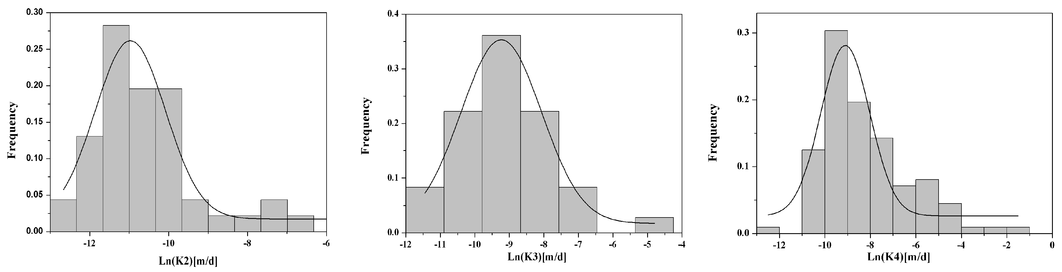
3.2. Probability Density Function of the Low Hydraulic Conductivity Field

The fitted parameters for these applied PDFs and the results of probability tests are listed in

Table 2. Fitting PDFs for the K samples from different layers.

Type of PDF		Second Layer	Third Layer	Fourth Layer
Normal	K–S	No	No	No
	A–D	No	No	No
	Fitted Parameters	$\mu$ = 9.55 × 10−5	$\mu$ = 5.63 × 10−4	$\mu$ = 0.0039
		$\sigma$ = 2.70 × 10−4c	$\sigma$ = 2.1 × 10−3	$\sigma$ = 0.0192
Log-normal	K–S	Yes	Yes	No
	A–D	Yes	Yes	No
	Fitted Parameters	$\mu$ = −10.59	$\mu$ = −9.08	$\mu$ = −8.25
		$\sigma$ = 1.33	$\sigma$ = 1.44	$\sigma$ = 1.91
Levy	K–S	Yes	Yes	Yes
	A–D	Yes	Yes	Yes
	Fitted Parameters	$\alpha$ = 0.46	$\alpha$ = 0.52	$\alpha$ = 0.52
		$\beta$ = 1	$\beta$ = 0.39	$\beta$ = 1
		$\gamma$ = 4.48 × 10−6	$\gamma$ = 2.10 × 10−5	$\gamma$ = 5.93 × 10−5
		$\delta$ = 7.47 × 10−6	$\delta$ = 5.30 × 10−5	$\delta$ = 2.10 × 10−6
Gamma	K–S	No	No	No
	A–D	No	No	No
	Fitted Parameters	a = 0.48	a = 0.41	a = 0.26
		b = 0.0002	b = 0.0014	b = 0.015
Weibull	K–S	No	Yes	No
	A–D	No	No	No
	Fitted Parameters	a = 0.0001	a = 0.0002	a = 0.0007
		b = 0.6	b = 0.56	b = 0.43

. The K data from the three layers were not confirmed to follow normal nor gamma distributions. Although Figure 2 shows graphical confirmation of a logarithmic normal distribution of hydraulic conductivities from the three layers, the fourth layer did not follow the log-normal distribution via the K–S nor A–D tests. Only the third layer followed the Weibull distribution via the K–S test. Moreover, all the low hydraulic conductivity values passed the probability of the Levy stable distribution.

Only the normal distribution could be considered to be symmetrically distributed in this study. All the results of the K–S and A–D tests revealed that the K values of low-permeable mediums had asymmetrical probability distributions, and also verified that the Levy stable distribution had more generality compared to the others. This is because the Levy stable distribution can serve as a family of PDFs, and four independent parameters of the Levy model provided better adaptability.

The Levy stable distribution is more flexible than the Gaussian distribution for fitting geophysical data obtained from strongly heterogeneous fields [22,31]. Herein, the K values from four layers were successfully modeled by the Levy stable distribution, and the four fitted Levy parameters are compared in Table 2. From layer 2 to layer 4, the Levy index $\alpha$ and scale parameter $\gamma$ increased from 0.46 to 0.52, and 4.48 × 10⁻⁶ to 5.93 × 10⁻⁵, respectively. As $\alpha$ decreases, the frequency of sudden large jumps in the random field increases [32]. The parameter $\gamma$ is known as the scale parameter. It is equal to half the variance when $\alpha$ = 2, and plays a similar role for $\alpha$ < 2 (i.e., it is a measure of the width of the distribution). As $\gamma$ increases, the magnitudes of the sudden large jumps increase [33]. The skewness parameter $\beta$ values for layers 2 and 4 were the same, equal to 1 (the maximum for this parameter), indicating extremely right-skewed distributions for these datasets. $\beta$ for layer 3 equaled 0.39, and the degree of skewness was weaker than for the other two layers. $\delta$, the shift parameter, represents the centering of the distribution, and it is equal to the mean of the distribution only when $\alpha$ > 1 and $\beta$ = 0. The differences of $\delta$ in Table 2 show the different centering of the four layers.

Based again on previous research [31,34], larger-scale property variations appear to be distributed normally, while smaller-scale variations follow the Levy stable distribution, and display an increased probability for sudden extreme events such as high or low K values. The measurement scale of NCG was controlled by the permeameter used (Φ: 61.8 mm × 40 mm). Hence, these K datasets could be categorized as small-scale. More extremes for K could be obtained through this permeameter. Another direct reason is that the K field of NCG was highly heterogeneous, as shown in Table 1 and Figure 3.

3.3. The Effects of K PDFs on Solute Transport

The studied case was an assumed 1-D cylinder filled with a homogenous isotropic porous medium, of infinite length. The conservative solute weighing 10 kg was injected to the cylinder. The cylinder cross-section was square at 10 cm × 10 cm. The effective porosity (n_e) was 0.3, and the longitudinal dispersion coefficient (D_L) was 0.05 m²/d. Although the porosity and dispersion coefficients were indeed of high variations for subsurface mediums, even for the silt and clay materials, we only focused the influence on the solute transport from the variation of K rather than the porosity and dispersion coefficients. The hydraulic gradient was set to a constant of 1.0, and the velocity (u) become a single-valued function of K; then the explicit expressions of t_p-K and C_p-K could be easily obtained from Equations (5) and (6). The monotonic variations, both of increasing C_p and decreasing t_p, with the increasing K value were observed from Figure 4. High t_p and low C_p values were consistent with the small K, and low t_p and high C_p values corresponded to a strong permeability of high K.

The statistical values of K for the silty clay medium from the third layer at the NCG site were applied to simulate the stochastic K datasets. As mentioned above, it can be concluded that the third layer of the medium followed log-normal and Levy stable distributions. The Monte Carlo method adopting the parameters from Table 2 was performed for the simulation of K. Afterwards, the peak time (t_p) and peak concentration (C_p) could be simulated by Equations (5) and (6).

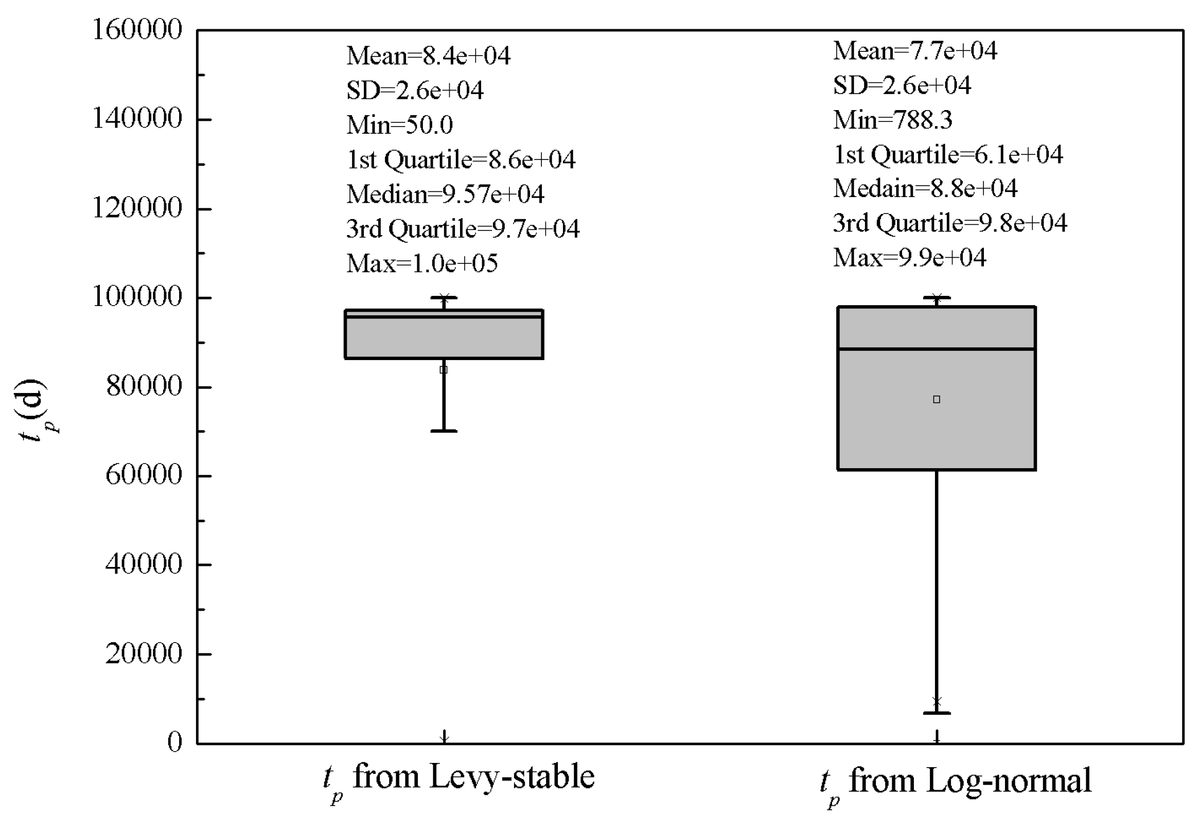
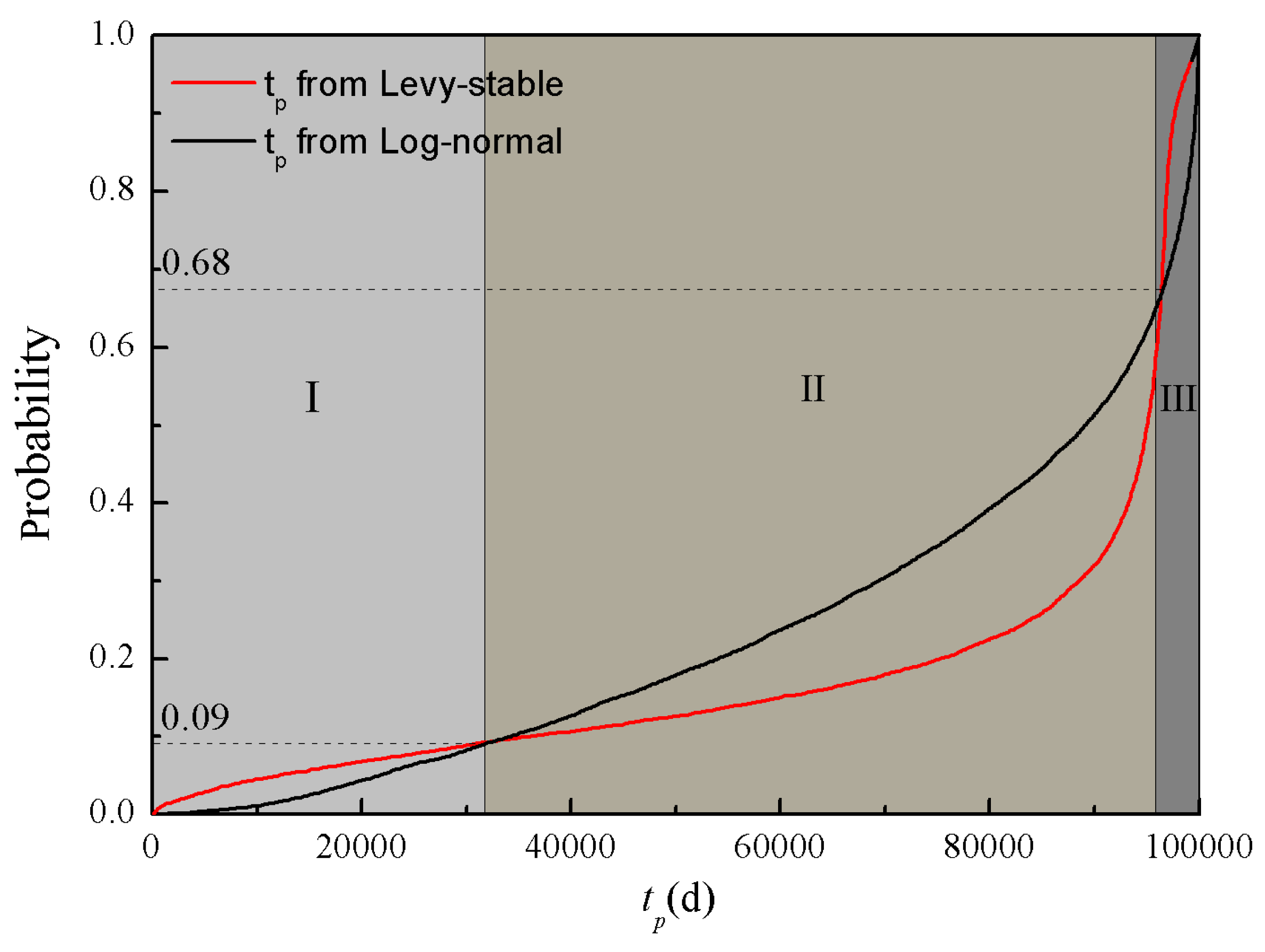
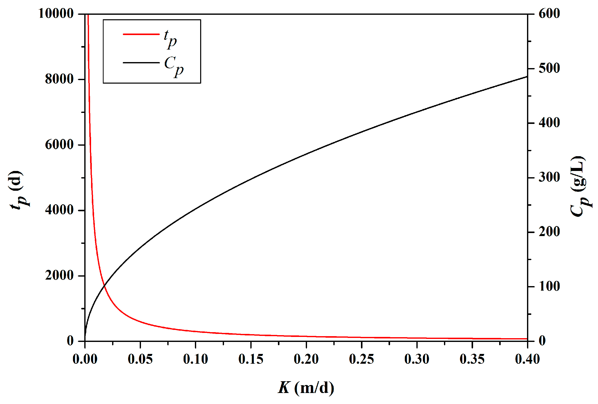
3.3.1. Effects of K PDFs on Peak Time

As shown in Figure 5, the range of peak times simulated by the Levy stable distribution (50.0 d, 1.0 × 10⁵ d) was a little greater than that simulated by the log-normal distribution (788.3 d, 9.9 × 10⁴ d). The minimum values especially between these two distributions were significantly different. This indicated that the Levy stable distribution could generate greater random values of K and then result in a smaller peak time. Additionally, the mean and median values of simulated peak time values from the Levy stable distribution (8.4 × 10⁴ d and 9.6 × 10⁴ d) were apparently greater than those of the log-normal distribution (7.7 × 10⁴ d and 8.8 × 10⁴ d). The interquartile ranges (IQRs) for the Levy-stable and log-normal distributions were 1.1 × 10⁴ d and 3.7 ×10⁴ d, respectively. From Figure 5, the simulation results of peak times from the Levy stable distribution are gathered in the area of greater value, and random numbers of K generated by the Levy stable distribution concentrate in the area of lower value. These results agreed with the high-peak and heavy-tail characteristics of the Levy stable distribution.

According to the differences of peak times and cumulative probabilities from the two distributions, the results shown in Figure 6 can be divided into three different sections. Section I includes the area of peak times less than 3.3 × 10⁴ d. Equation (4) explicitly indicates the negative correlation between peak time and flow velocity. In this study, velocity (u) was proportional to K through the assumed 1-D model, and the peak time (t_p) and K had a negative correlation. Section I reflects the simulation result when K was relatively large. As shown in Figure 5, the results calculated by the Levy stable distribution indicated that the probability of small peak time events (red line) was clearly higher than that calculated by the log-normal distribution (black line).

The peak time of Section II was between 3.3 × 10⁴ d and 9.6 × 10⁴ d, and Section II is shown as the middle part of Figure 5. According to the correlation between the peak time and K mentioned above, this section corresponds to the range for which K was moderate (greater than that in Section I and less than that in Section III). The simulation results indicated that the log-normal distribution achieved a higher probability than the Levy stable distribution. The probability of random events with moderate peak times simulated by the Levy stable distribution was less than that for the log-normal distribution. The peak time of Section III was the highest, representing the smallest K. The simulation results indicated that the probability of high peak time events simulated by the Levy stable distribution was larger than for the log-normal distribution.

In conclusion, under the Levy stable distribution, the distribution of t_p calculated by the simple analytical model had more non-uniform characteristics. The probabilities of a greater peak time occurring (Section I) and smaller values occurring (Section III) were both larger than for under the widely used log-normal distribution. However, the comparison of moderate peak time events (Section II) revealed that the probability calculated by the log-normal distribution was clearly greater than that by the Levy stable distribution. Our results indicate that simulated t_p values from log-normally-distributed K are likely ranged within the medium level, and the Levy stable distribution can produce higher or lower extremes much more easily.

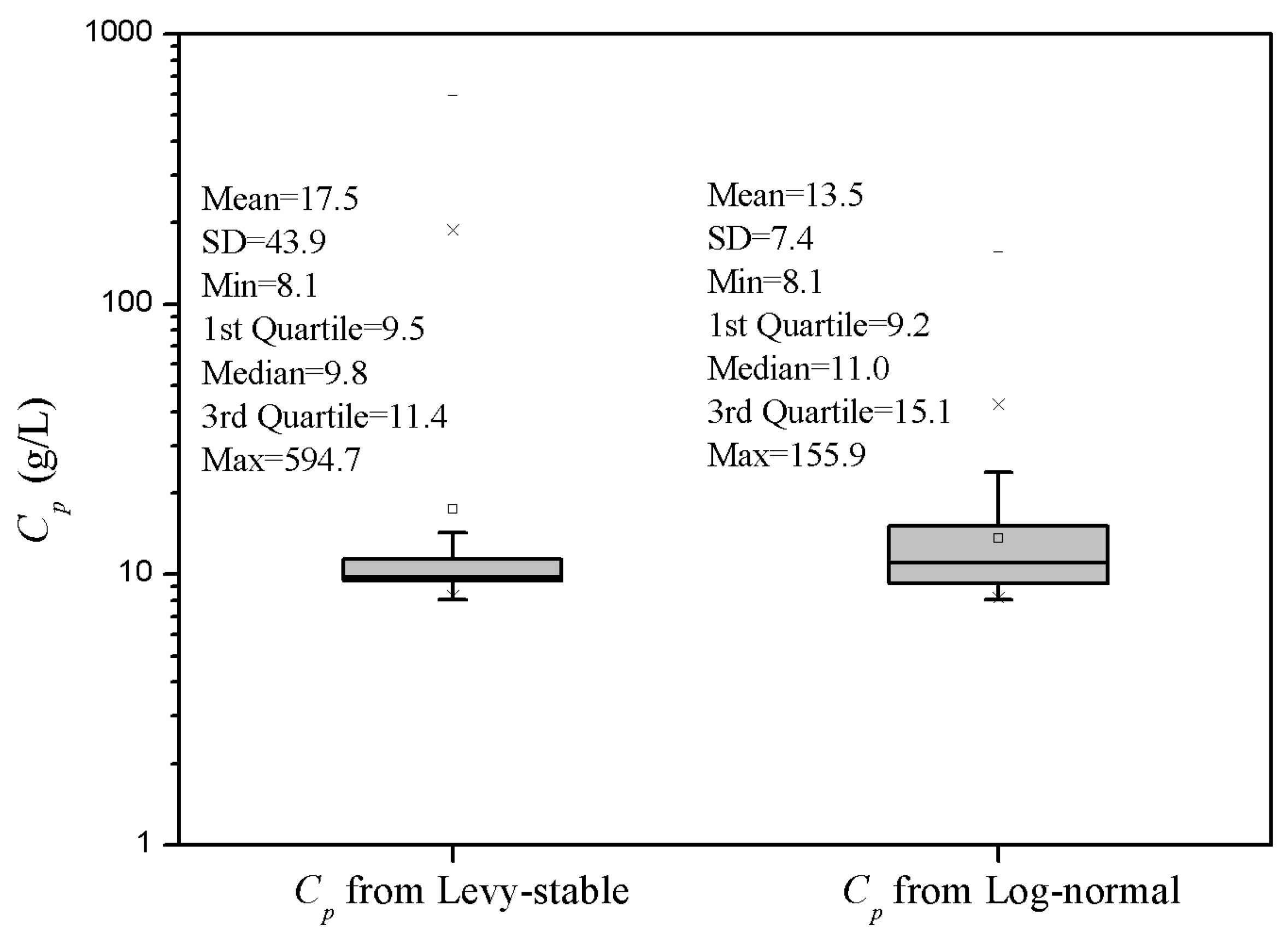
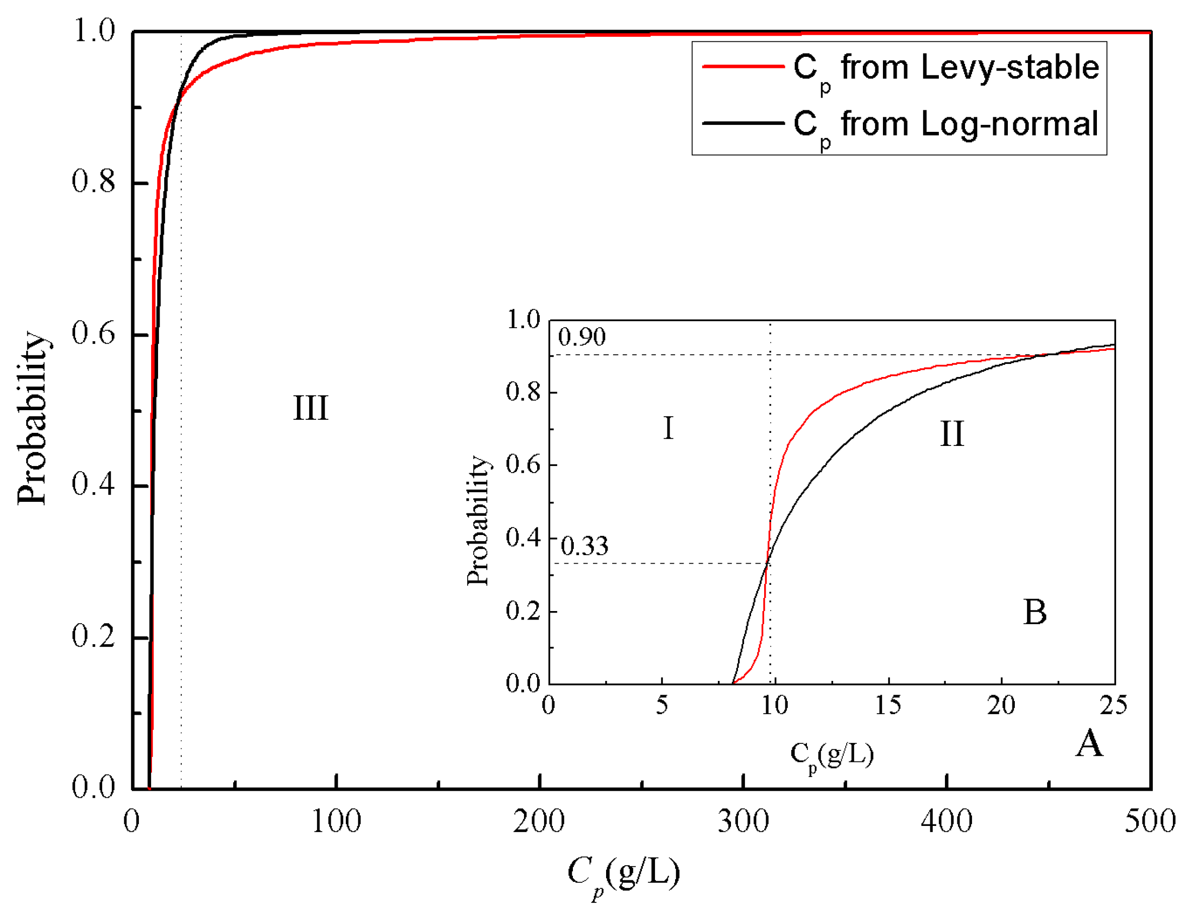
3.3.2. Effects of K PDFs on Peak Concentration

As shown in Figure 7, the range of peak concentrations (C_p) simulated by the Levy stable distribution (8.1 g/L, 594.7 g/L) was significantly greater than that simulated by the log-normal distribution (8.1 g/L, 155.9 g/L). The maximum values between these two distributions were significantly different. The average value of the simulated peak concentration from the Levy stable distribution (17.5 g/L) was slightly greater than that from the log-normal distribution (13.5 g/L). However, the median of the Levy stable distribution (9.8 g/L) was slightly less than the counterpart of the log-normal distribution (11.0 g/L). Although the standard deviation of C_p from the Levy stable distribution (43.9 g/L) was much greater than that from the log-normal distribution (7.4 g/L), the Levy stable distribution could generate a concentrated C_p (IQR = 1.9 g/L) compared with the log-normal distribution (IQR = 5.9 g/L), as seen from the shorter box in Figure 7.

Similarly to the cumulative frequency of t_p shown in Figure 6, three different sections of C_p are discriminated in Figure 8 (Sections I and II are zoomed in Figure 8B). According to Equation (3), the peak concentration (C_p) had a positive correlation with the flow velocity (u). Since the flow velocity (u) had a positive correlation with the hydraulic conductivity (K), a positive correlation between C_p and K could be inferred. The cumulative probability of random events in Sections I and II contributed approximately 90% of all random samples. In Sections I and II, the difference of cumulative frequency distributions of C_p under two different distributions was small, as shown by Figure 8A. Approximately 90% of simulated peak concentrations were located in the range of 8–25 g/L for both of the two distributions. In Section III, the peak concentration from the log-normal distribution achieved the highest value of 155.9 g/L, and the greater C_p (>155.9 g/L) only appeared under the assumption of Levy-stable-distributed K. The distribution of C_p under the Levy stable distribution was much flatter than that under the log-normal distribution. The Levy stable distribution had better performance to simulate extreme conditions and to reveal the heavy-tailed characteristic of hydraulic conductivity, especially.

4. Conclusions

The hydraulic properties of an aquifer vary irregularly in 3-D space, as a general rule. In this study, a comprehensive field investigation of the NCG site was performed. The lithology of NCG is dominated by silty clay and clay. In total, 212 falling head permeameter tests were performed to investigate the characteristics of hydraulic conductivity for the silty clay site. The statistical patterns of hydraulic conductivity were analyzed, and the probability distributions of K were tested by five models.

One of our main findings was that the hydraulic conductivity of a low hydraulic conductivity medium, such as silty clay, likely comes from the Levy stable distribution. The log-normal distribution could also cover most of the low hydraulic conductivity, and the Weibull distribution could describe part of the samples of clay, but neither the normal distribution nor the gamma distribution could fit any of the experimental probability curves of the NCG site. Therefore, the Levy stable distribution is recommended for depicting the statistics of a low-K field.

The effects of the probability distribution of the hydraulic conductivity on the solute transport were analyzed using a simple analytical model. The peak concentration and its corresponding time were selected to represent the transport process. The Levy stable distribution was apt to generate the extremes of the solute transport (higher peak concentration and lower peak time), compared with the widely used log-normal distribution. These results have a great guiding significance for describing the migration characteristics of contaminations in underground mediums.

References

1. Freeze, R.A.; Cherry, J.A. Groundwater; Prentice Hall: Englewood Cliffs, NJ, USA, 1979. [Google Scholar]
2. Kohlbecker, M.V.; Wheatcraft, S.W.; Meerschaert, M.M. Heavy-tailed log hydraulic conductivity distributions imply heavy-tailed log velocity distributions. Water Resour. Res. 2006, 42, W04411. [Google Scholar] [CrossRef]
3. Wang, K.; Huang, G. Effect of permeability variations on solute transport in highly heterogeneous porous media. Adv. Water Resour. 2011, 34, 671–683. [Google Scholar] [CrossRef]
4. Schertzer, D.; Lovejoy, S. Physical modeling and analysis of rain and clouds by anisotropic scaling multiplicative processes. J. Geophys. Res. 1987, 92, 9693–9714. [Google Scholar] [CrossRef]
5. Freeze, R.A. A stochastic-conceptual analysis of one-dimensional groundwater flow in nonuniform homogeneous media. Water Resour. Res. 1975, 11, 725–741. [Google Scholar] [CrossRef]
6. Bjerg, P.L.; Hinsby, K.; Christensen, T.H.; Gravesen, P. Spatial variability of hydraulic conductivity of an unconfined sandy aquifer determined by a mini slug test. J. Hydrol. 1992, 136, 107–122. [Google Scholar] [CrossRef]
7. Hess, K.M.; Wolf, S.H.; Celia, M.A. Large-scale natural gradient tracer test in sand and gravel, cape cod, massachusetts: 3. Hydraulic conductivity variability and calculated macrodispersivities. Water Resour. Res. 1992, 28, 2011–2027. [Google Scholar] [CrossRef]
8. Turcke, M.A.; Kueper, B.H. Geostatistical analysis of the borden aquifer hydraulic conductivity field. J. Hydrol. 1996, 178, 223–240. [Google Scholar] [CrossRef]
9. Sudicky, E.A. A natural gradient experiment on solute transport in a sand aquifer: Spatial variability of hydraulic conductivity and its role in the dispersion process. Water Resour. Res. 1986, 22, 2069–2082. [Google Scholar] [CrossRef]
10. Woodbury, A.D.; Sudicky, E.A. The geostatistical characteristics of the borden aquifer. Water Resour. Res. 1991, 27, 533–546. [Google Scholar] [CrossRef]
11. Cheng, C.; Song, J.; Chen, X.; Wang, D. Statistical distribution of streambed vertical hydraulic conductivity along the platte river, nebraska. Water Resour. Manag. 2011, 25, 265–285. [Google Scholar] [CrossRef]
12. Sánchez-Vila, X.; Carrera, J.; Girardi, J.P. Scale effects in transmissivity. J. Hydrol. 1996, 183, 1–22. [Google Scholar] [CrossRef]
13. Hyun, Y. Multiscale Anaylses of Permeability in Porous and Fractured Media. Ph.D. Thesis, The University of Arizona, Tucson, AZ, USA, 2002. [Google Scholar]
14. Rehfeldt, K.R.; Boggs, J.M.; Gelhar, L.W. Field study of dispersion in a heterogeneous aquifer: 3. Geostatistical analysis of hydraulic conductivity. Water Resour. Res. 1992, 28, 3309–3324. [Google Scholar] [CrossRef]
15. Vereecken, H.; Döring, U.; Hardelauf, H.; Jaekel, U.; Hashagen, U.; Neuendorf, O.; Schwarze, H.; Seidemann, R. Analysis of solute transport in a heterogeneous aquifer: The krauthausen field experiment. J. Contam. Hydrol. 2000, 45, 329–358. [Google Scholar] [CrossRef]
16. Bagarello, V.; Iovino, M.; Elrick, D. A simplified falling-head technique for rapid determination of field-saturated hydraulic conductivity. Soil Sci. Soc. Am. J. 2004, 68, 66–73. [Google Scholar] [CrossRef]
17. Dagan, G. Flow and Transport in Porous Formations; Springer: Berlin/Heidelberg, Germany, 1989. [Google Scholar]
18. Liang, J.; Zeng, G.; Guo, S.; Li, J.; Wei, A.; Shi, L.; Li, X. Uncertainty analysis of stochastic solute transport in a heterogeneous aquifer. Environ. Eng. Sci. 2009, 26, 359–368. [Google Scholar] [CrossRef]
19. Ye, B.; Zhang, Z.; Mao, T. Petroleum hydrocarbon in surficial sediment from rivers and canals in Tianjin, China. Chemosphere 2007, 68, 140–149. [Google Scholar] [CrossRef] [PubMed]
20. Cong, S. Probability and Statistical Methods in Water Science and Technology; Science Press: Beijing, China, 2010. [Google Scholar]
21. Painter, S. Flexible scaling model for use in random field simulation of hydraulic conductivity. Water Resour. Res. 2001, 37, 1155–1163. [Google Scholar] [CrossRef]
22. Yang, C.-Y.; Hsu, K.-C.; Chen, K.-C. The use of the levy-stable distribution for geophysical data analysis. Hydrogeol. J. 2009, 17, 1265–1273. [Google Scholar] [CrossRef]
23. Liang, Y.; Chen, W. A survey on computing lévy stable distributions and a new matlab toolbox. Signal Process. 2013, 93, 242–251. [Google Scholar] [CrossRef]
24. Nolan, J.P. Parameterizations and modes of stable distributions. Stat. Probab. Lett. 1998, 38, 187–195. [Google Scholar] [CrossRef]
25. Helsel, D.R.; Hirsch, R.M. Statistical Methods in Water Resources Techniques of Water Resources Investigations; U.S. Geological Survey: Reston, VA, USA, 2002; Volume 4, p. 522. [Google Scholar]
26. Arnold, T.B.; Emerson, J.W. Nonparametric goodness-of-fit tests for discrete null distributions. R J. 2011, 3, 34–39. [Google Scholar]
27. Stephens, M.A. Edf statistics for goodness of fit and some comparisons. J. Am. Stat. Assoc. 1974, 69, 730–737. [Google Scholar] [CrossRef]
28. De Jong, G.D.J. Longitudinal and transverse diffusion in granular deposits. In Soil Mechanics and Transport in Porous Media: Selected works of g. De Josselin de Jong; Schotting, R.J., van Duijn, H.C.J., Verruijt, A., Eds.; Springer: Dordrecht, The Netherlands, 2006; pp. 261–268. [Google Scholar]
29. Gégo, E.L.; Johnson, G.S.; Hankins, M. An evaluation of methodologies for the generation of stochastic hydraulic conductivity fields in highly heterogeneous aquifers. Stoch. Environ. Res. Risk Assess. 2001, 15, 47–64. [Google Scholar] [CrossRef]
30. Teatini, P.; Ferronato, M.; Gambolati, G.; Baù, D.; Putti, M. Anthropogenic venice uplift by seawater pumping into a heterogeneous aquifer system. Water Resour. Res. 2010, 46, W11547. [Google Scholar] [CrossRef]
31. Painter, S. Stochastic interpolation of aquifer properties using fractional lévy motion. Water Resour. Res. 1996, 32, 1323–1332. [Google Scholar] [CrossRef]
32. Tennekoon, L.; Boufadel, M.C.; Lavallee, D.; Weaver, J. Multifractal anisotropic scaling of the hydraulic conductivity. Water Resour. Res. 2003, 39, SBH 8-1. [Google Scholar] [CrossRef]
33. Boufadel, M.C.; Lu, S.L.; Molz, F.J.; Lavallee, D. Multifractal scaling of the intrinsic permeability. Water Resour. Res. 2000, 36, 3211–3222. [Google Scholar] [CrossRef]
34. Liu, H.H.; Molz, F.J. Multifractal analyses of hydraulic conductivity distributions. Water Resour. Res. 1997, 33, 2483–2488. [Google Scholar] [CrossRef]
Figure 1. Spatial distribution of boreholes (A), and the 3D geological structure (B).
Water 09 00466 g001
Figure 2. Frequency histograms of K for three layers, and the normal curves.
Water 09 00466 g002
Figure 3. Hydraulic conductivities of mediums, decreasing via elevation.
Water 09 00466 g003
Figure 4. Variation curves of tp and Cp versus the corresponding K values.
Water 09 00466 g004
Figure 5. Boxplot of tp using K values followed Levy stable and log-normal distributions.
Water 09 00466 g005
Figure 6. Cumulative frequency distributions of tp from Levy stable and log-normal distribution K values.
Water 09 00466 g006
Figure 7. Boxplot of Cp using K values following Levy stable and log-normal distributions.
Water 09 00466 g007
Figure 8. Cumulative frequency distribution of Cp from Levy stable and log-normal distribution K values (8A shows the full extent and 8B shows the part of Cp less than 25 g/L).
Water 09 00466 g008