
Local Climate Change and the Impacts on Hydrological Processes in an Arid Alpine Catchment in Karakoram

 ,
,
Abstract
:1. Introduction
2. Study Area and Data
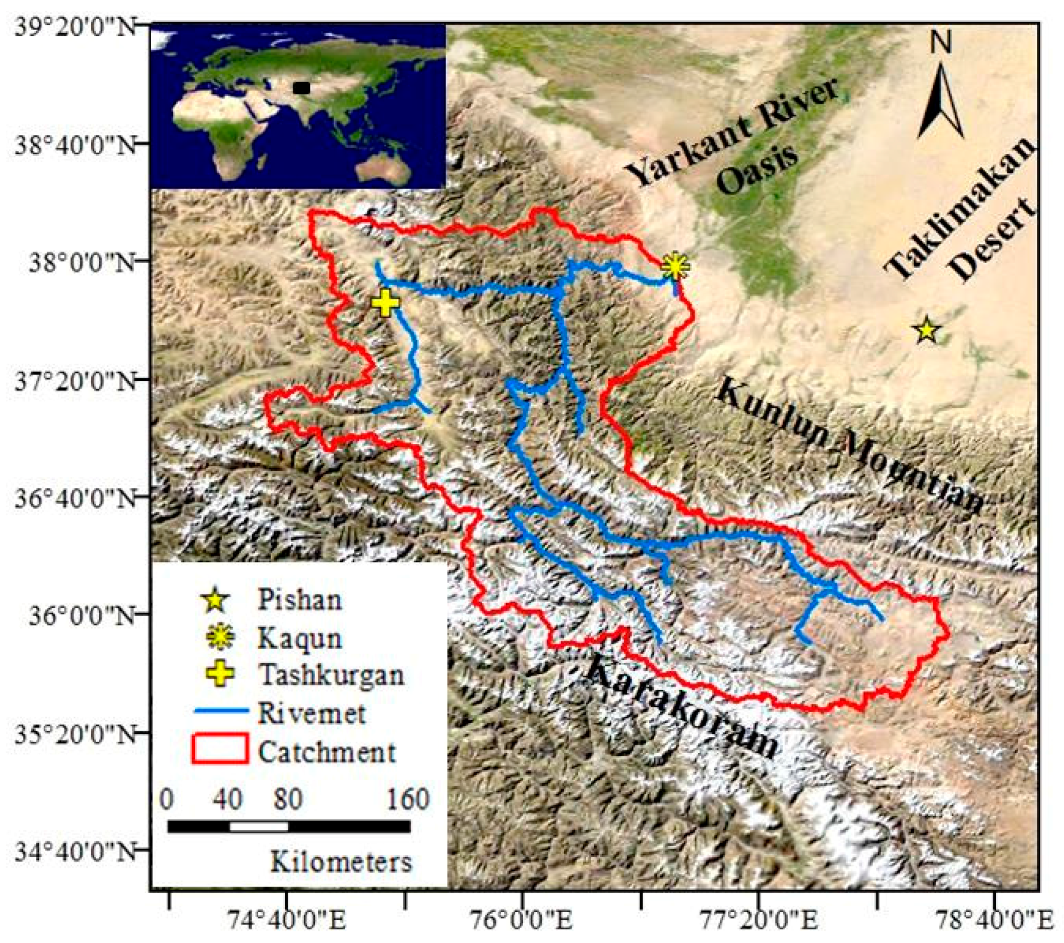
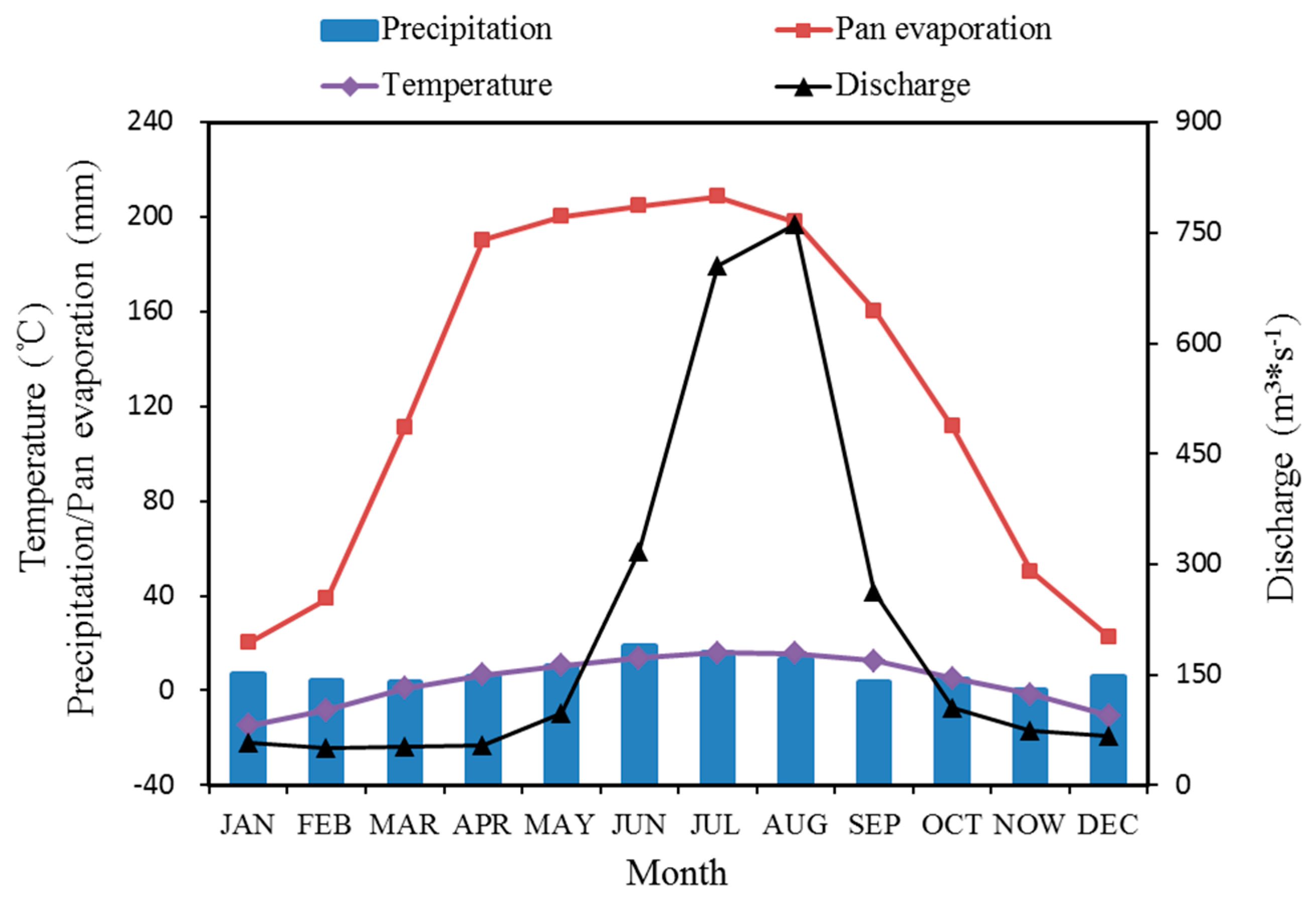
2.1. Study Area
2.2. Data
3. Methodology
3.1. Modified QPM for Precipitation
- Calculate the number of rainy days () and quantiles of each precipitation event () in the observed time series of HP;
- Interpolate and in the GCMs, maintaining the same quantile i with throughout the linear method, then calculate based on Equation (3) and ;
- Obtain the future precipitation intensity at each quantile i (), formulated as ;
- Obtain the number of future rainy days (), formulated as ;
- Count the existing number of rainy days () for which quantile i is not more than 0.01 in step 3;
- Calculate the expected number of rainy days () for which quantile i is not more than 0.01 based on the result in step 4, formulated as If , (), no rainy days should be replaced in step 3, and the precipitation of added rainy days is equal to the average value of existing rainy days . Perform the above subtraction and round the difference between to the nearest integer;
- Sequentially repeat steps 5 and 6 at the other quantiles (0.05, 0.1, 0.2, 0.3, 0.4, 0.5, 0.6, 0.7, 0.8 and 0.9) until the number of rainy days in step 3 is equal to .
3.2. Delta Method for Temperature
3.3. Hydrological Modelling
4. Results and Discussion
4.1. Future Climate Change
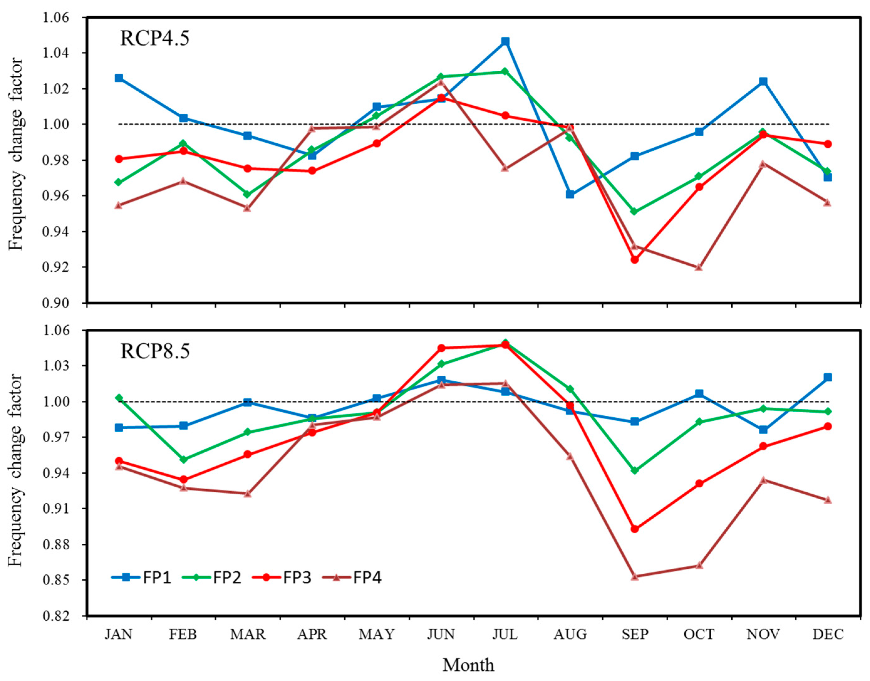
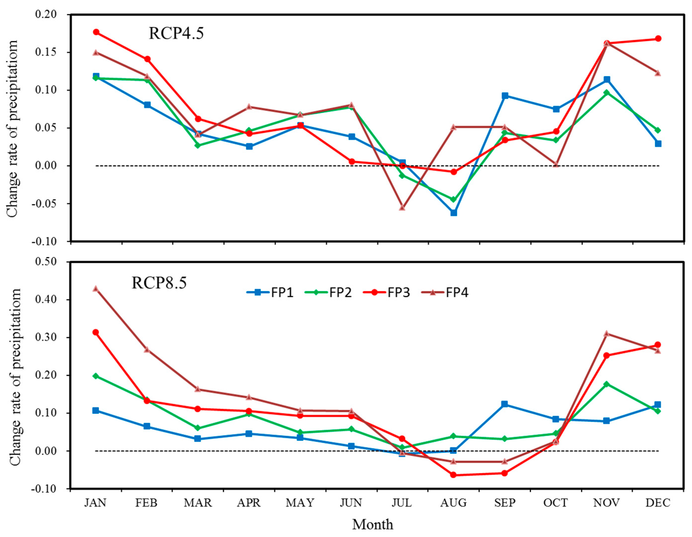
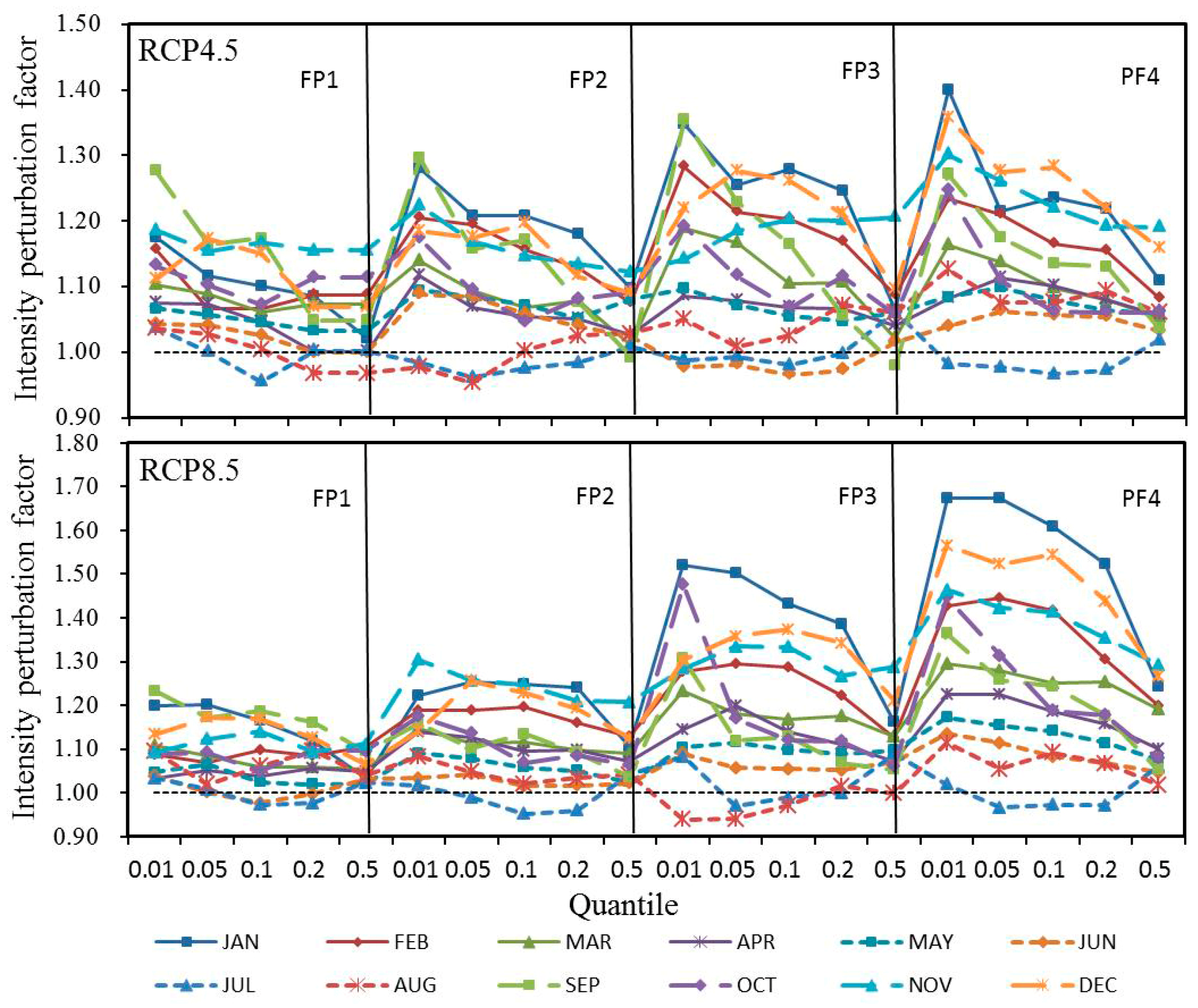
4.1.1. Precipitation
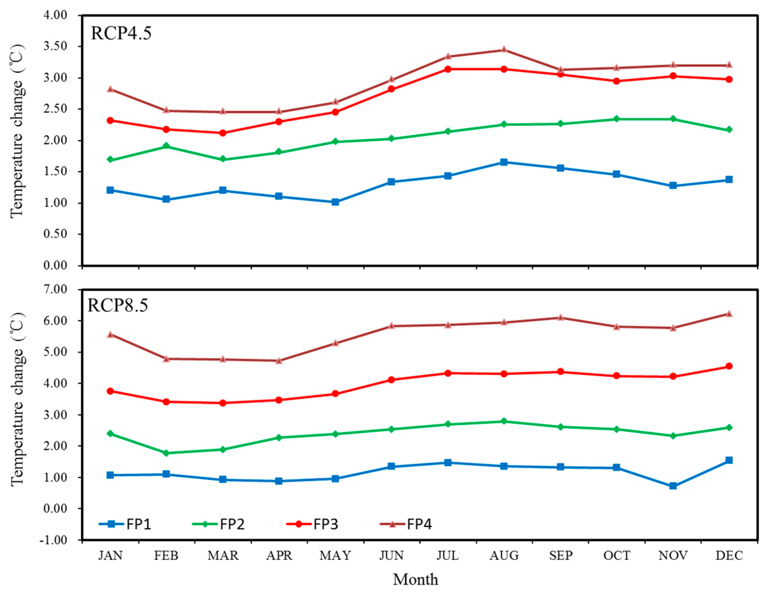
4.1.2. Temperature
4.2. Water Balance
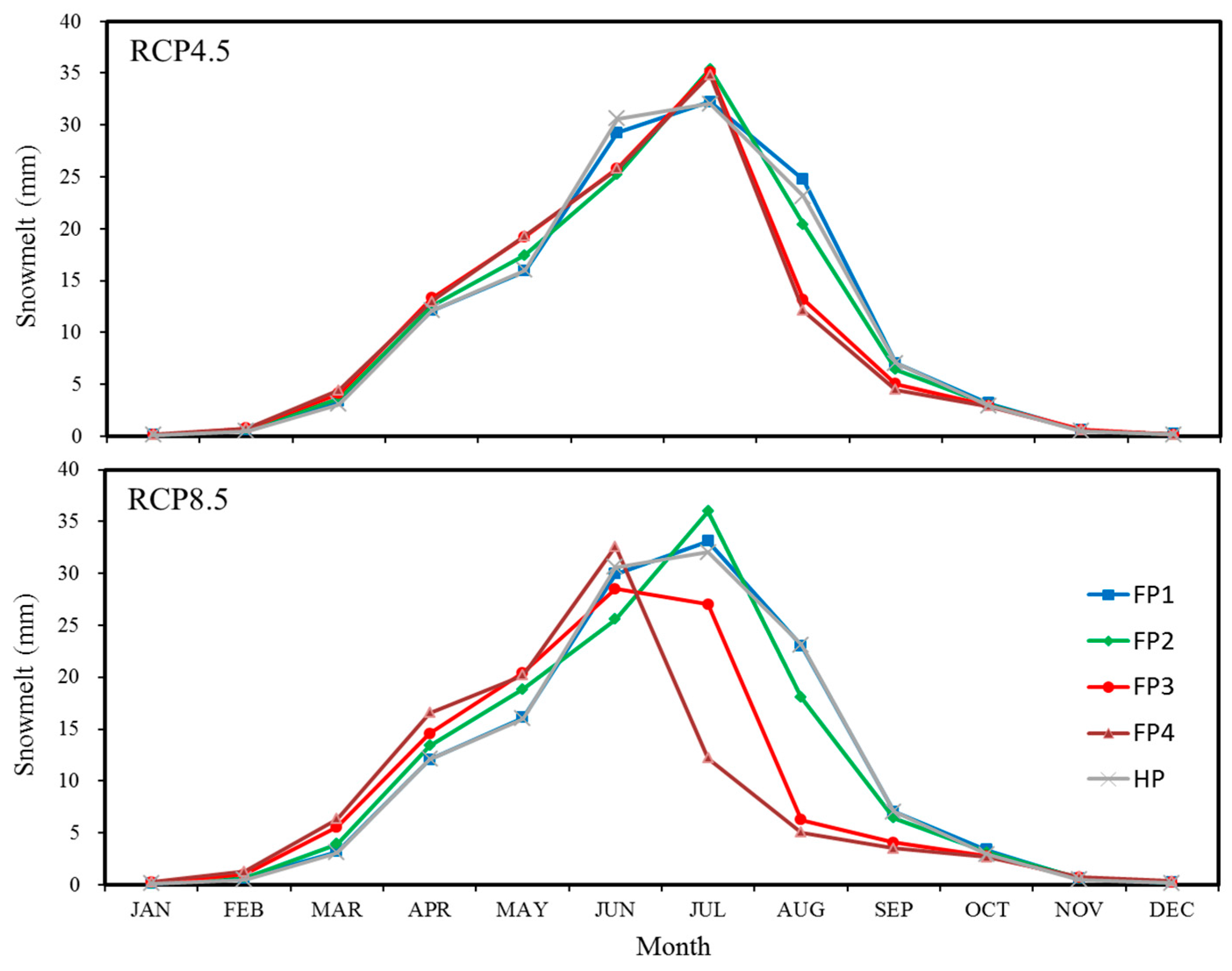
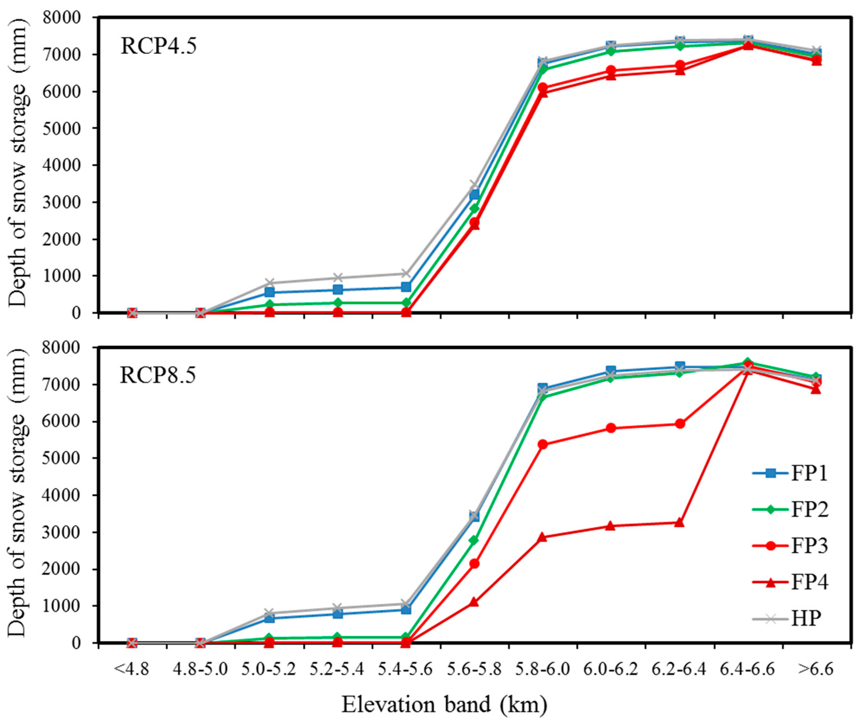
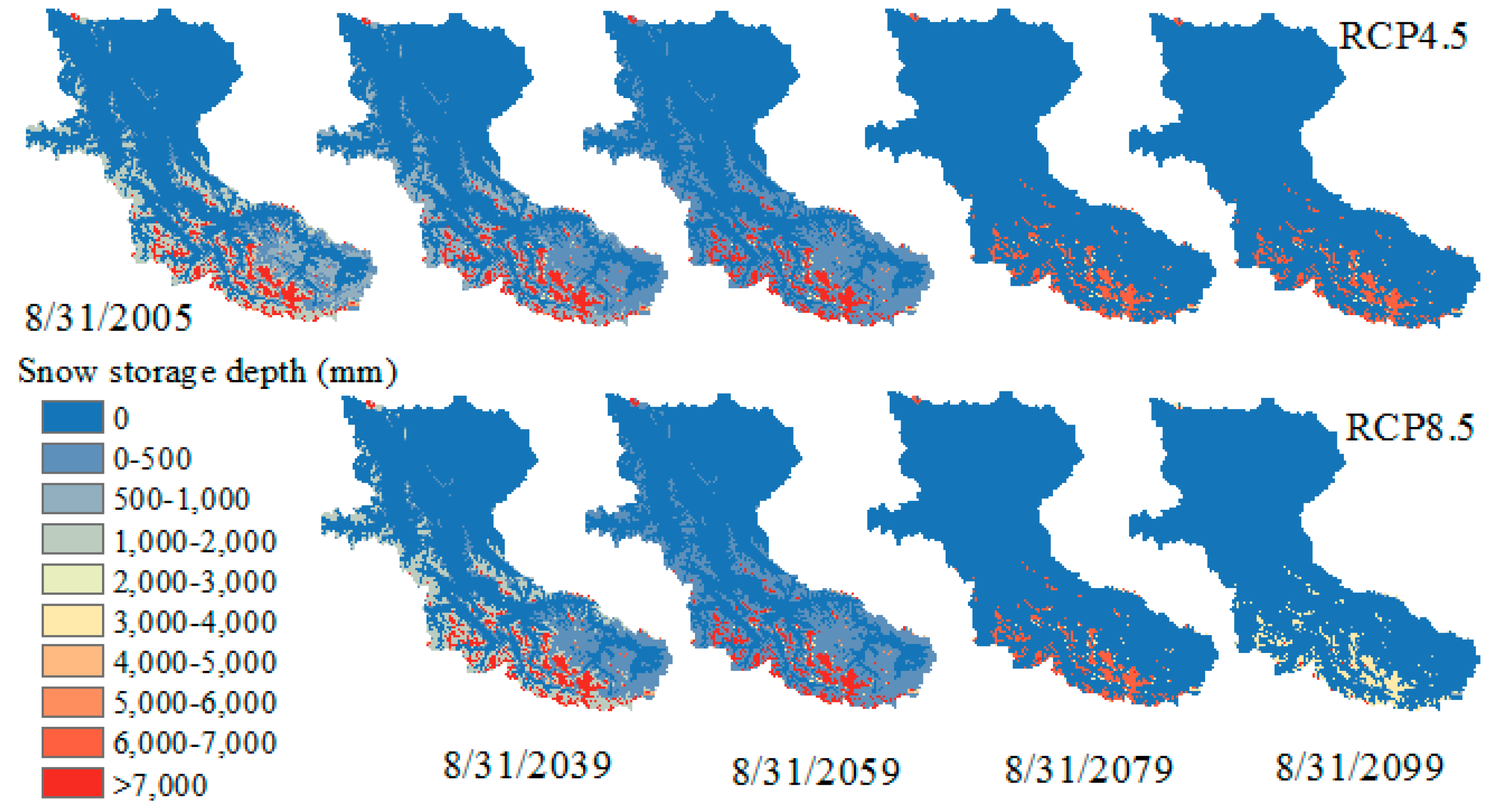
4.2.1. Snow
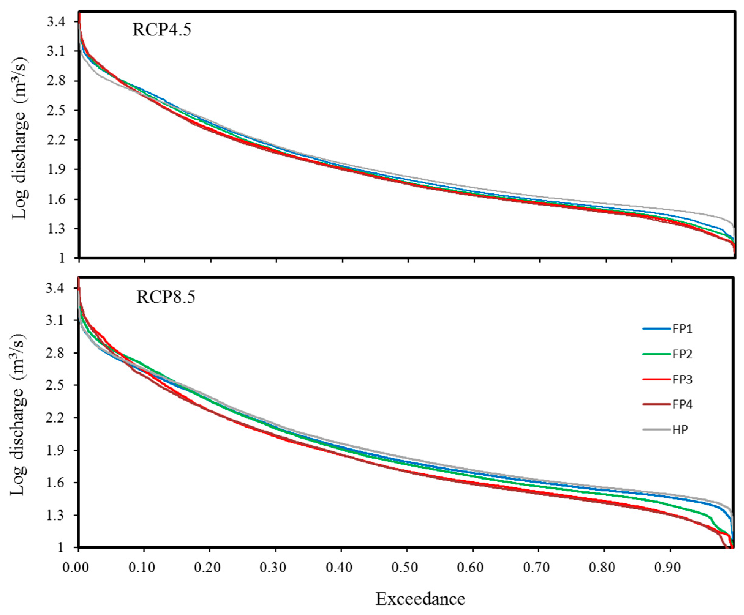
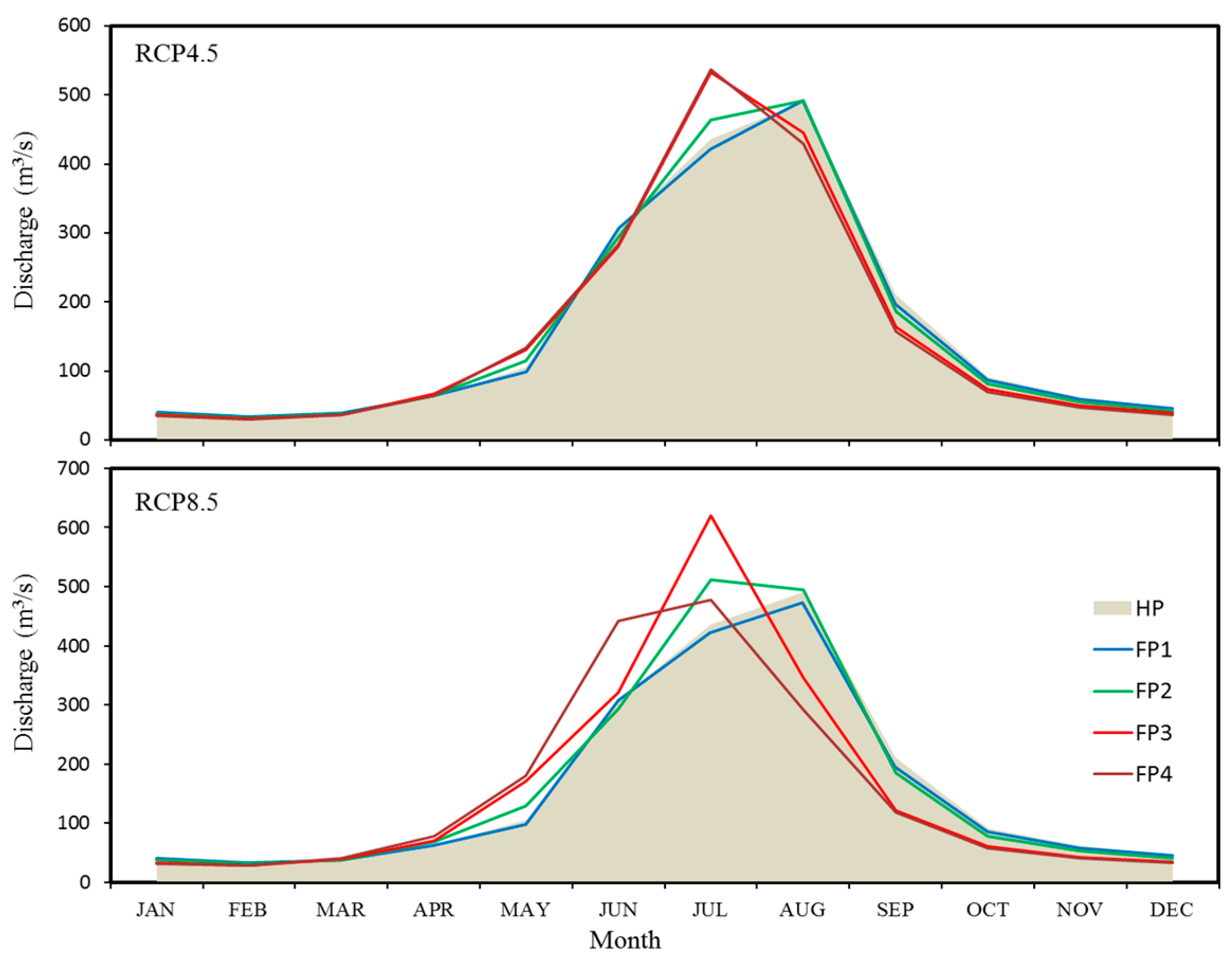
4.2.2. Streamflow
5. Conclusions
Acknowledgments
Author Contributions
Conflicts of Interest
References
- IPCC. Climate Change 2013: The Physical Science Basis. Contribution of Working Group I to the Fifth Assessment Report of IPCC; Cambridge University Press: Cambridge, UK; New York, USA, 2013. [Google Scholar] [CrossRef]
- Chen, Y.; Takeuchi, K.; Xu, C.; Chen, Y.; Xu, Z. Regional climate change and its effects on river runoff in the Tarim basin, China. Hydrol. Process. 2006, 20, 2207–2216. [Google Scholar] [CrossRef]
- Guo, L.; Li, L. Variation of the proportion of precipitation occurring as snow in the Tian Shan mountains, China. Int. J. Climatol. 2015, 35, 1379–1393. [Google Scholar] [CrossRef]
- Huss, M.; Farinotti, D.; Bauder, A.; Funk, M. Modelling runoff from highly glacierized alpine drainage basins in a changing climate. Hydrol. Process. 2008, 22, 3888–3902. [Google Scholar] [CrossRef]
- Springer, C.; Matulla, C.; Schöner, W.; Steinacker, R.; Wagner, S. Downscaled GCM projections of winter and summer mass balance for Central European glaciers (2000–2100) from ensemble simulations with ECHAM5-MPIOM. Int. J. Climatol. 2013, 33, 1270–1279. [Google Scholar] [CrossRef]
- Barontini, S.; Grossi, G.; Kouwen, N.; Maran, S.; Scaroni, P.; Ranzi, R. Impacts of climate change scenarios on runoff regimes in the southern Alps. Hydrol. Earth Syst. Sci. 2009, 6, 3089–3141. [Google Scholar] [CrossRef]
- Liu, S.Y.; Yong, Z.; Song, Z.Y.; Yong, D. Estimation of glacier runoff and future trends in the Yangtze River source region, China. J. Glaciol. 2009, 55, 353–362. [Google Scholar] [CrossRef]
- Jeelani, G.; Feddema, J.J.; Veen, C.J.; Stearns, L. Role of snow and glacier melt in controlling river hydrology in Liddar watershed (western Himalaya) under current and future climate. Water Resour. Res. 2012, 48, 12508. [Google Scholar] [CrossRef]
- Bavay, M.; Grünewald, T.; Lehning, M. Response of snow cover and runoff to climate change in high Alpine catchments of eastern Switzerland. Adv. Water Resour. 2013, 55, 4–16. [Google Scholar] [CrossRef]
- Su, F.; Zhang, L.; Ou, T.; Chen, D.; Yao, T.; Tong, K.; Qi, Y. Hydrological response to future climate changes for the major upstream river basins in the Tibetan Plateau. Glob. Planet. Chang. 2016, 136, 82–95. [Google Scholar] [CrossRef]
- Immerzeel, W.W.; van Beek, L.P.; Bierkens, M.F. Climate change will affect the Asian water towers. Science 2010, 328, 1382–1385. [Google Scholar] [CrossRef] [PubMed]
- Calanca, P.; Roesch, A.; Jasper, K.; Wild, M. Global warming and the summertime evapotranspiration regime of the Alpine region. Clim. Chang. 2006, 79, 65–78. [Google Scholar] [CrossRef]
- Thompson, J.R.; Green, A.J.; Kingston, D.G. Potential evapotranspiration-related uncertainty in climate change impacts on river flow: An assessment for the Mekong River basin. J. Hydrol. 2014, 510, 259–279. [Google Scholar] [CrossRef]
- Roosmalen, L.V.; Sonnenborg, T.O.; Jensen, K.H. Impact of climate and land use change on the hydrology of a large-scale agricultural catchment. Water Resour. Res. 2009, 45, 150–164. [Google Scholar] [CrossRef]
- Chen, Y.; Xu, C.; Chen, Y.; Li, W.; Liu, J. Response of glacial-lake outburst floods to climate change in the Yarkant River basin on northern slope of Karakoram mountains, China. Quat. Int. 2010, 226, 75–81. [Google Scholar] [CrossRef]
- Xu, H.; Zhou, B.; Song, Y. Impacts of climate change on headstream runoff in the Tarim River Basin. Hydrol. Res. 2010, 42, 20–29. [Google Scholar] [CrossRef]
- Zhang, Q.; Xu, C.Y.; Tao, H.; Jiang, T.; Chen, Y.D. Climate changes and their impacts on water resources in the arid regions: A case study of the Tarim River basin, China. Stoch. Environ. Res. Risk Assess. 2010, 24, 349–358. [Google Scholar] [CrossRef]
- Xu, C.; Chen, Y.; Chen, Y.; Zhao, R.; Ding, H. Responses of surface runoff to climate change and human activities in the arid region of central Asia: A case study in the Tarim River basin, China. Environ. Manag. 2013, 51, 926–938. [Google Scholar] [CrossRef] [PubMed]
- Zhang, S.; Gao, X.; Zhang, X.; Hagemann, S. Projection of glacier runoff in Yarkant River basin and Beida River basin, Western China. Hydrol. Process. 2012, 26, 2773–2781. [Google Scholar] [CrossRef]
- Onyutha, C.; Tabari, H.; Rutkowska, A.; Nyeko-Ogiramoi, P.; Willems, P. Comparison of different statistical downscaling methods for climate change rainfall projections over the Lake Victoria basin considering CMIP3 and CMIP5. J. Hydrol. Environ. Res. 2016, 12, 31–45. [Google Scholar] [CrossRef]
- Min, S.K.; Zhang, X.; Zwiers, F.W.; Hegerl, G.C. Human contribution to more-intense precipitation extremes. Nature 2011, 470, 378–381. [Google Scholar] [CrossRef] [PubMed]
- Salathé, E.P.; Hamlet, A.F.; Mass, C.F.; Lee, S.; Stumbaugh, M.; Steed, R. Estimates of twenty-first-century flood risk in the Pacific Northwest based on regional climate model simulations. J. Hydrometeorol. 2014, 15, 1881–1899. [Google Scholar] [CrossRef]
- Quintana Seguí, P.; Ribes, A.; Martin, E.; Habets, F.; Boé, J. Comparison of three downscaling methods in simulating the impact of climate change on the hydrology of Mediterranean basins. J. Hydrol. 2010, 383, 111–124. [Google Scholar] [CrossRef]
- Liu, T.; Willems, P.; Pan, X.L.; Bao, A.M.; Chen, X.; Veroustraete, F.; Dong, Q.H. Climate change impact on water resource extremes in a headwater region of the Tarim basin in China. Hydrol. Earth Syst. Sci. 2011, 15, 3511–3527. [Google Scholar] [CrossRef]
- Taye, M.T.; Ntegeka, V.; Ogiramoi, N.P.; Willems, P. Assessment of climate change impact on hydrological extremes in two source regions of the Nile River Basin. Hydrol. Earth Syst. Sci. 2011, 15, 209–222. [Google Scholar] [CrossRef]
- Willems, P.; Vrac, M. Statistical precipitation downscaling for small-scale hydrological impact investigations of climate change. J. Hydrol. 2011, 402, 193–205. [Google Scholar] [CrossRef]
- Ntegeka, V.; Baguis, P.; Roulin, E.; Willems, P. Developing tailored climate change scenarios for hydrological impact assessments. J. Hydrol. 2014, 508, 307–321. [Google Scholar] [CrossRef]
- Lettenmaier, D.P.; Wood, A.W.; Palmer, R.N.; Wood, E.F.; Stakhiv, E.Z. Water resources implications of global warming: A U.S regional perspective. Clim. Chang. 1999, 43, 537–579. [Google Scholar] [CrossRef]
- Middelkoop, H.; Daamen, K.; Gellens, D.; Grabs, W.; Kwadijk, J.C.; Lang, H.; Parment, B.A.; Schadler, B.; Schulla, J.; Wilke, K. Impact of ClimateChange on the Hydrological Regime and Water Resources Management in the Rhine Basin. Clim. Chang. 2001, 49, 105–128. [Google Scholar] [CrossRef]
- Ntegeka, V.; Willems, P.; Baguis, P.; Roulin, E. Climate Change Impact on Hydrological Extremes along Rivers and Urban Drainage Systems in Belgium; Summary Report Phase 1: Literature Review and Development of Climate Change Scenarios: Belgian Science Policy-SSD Research Programme, CCI-HYDR Project; KU Leuven: Leuven/Brussels, Belgium, 2008. [Google Scholar]
- Chen, J.; Brissette, F.P.; Leconte, R. Uncertainty of downscaling method in quantifying the impact of climate change on hydrology. J. Hydrol. 2011, 401, 190–202. [Google Scholar] [CrossRef]
- Ghosh, S.; Katkar, S. Modeling uncertainty resulting from multiple downscaling methods in assessing hydrological impacts of climate change. Water Resour. Manag. 2012, 26, 3559–3579. [Google Scholar] [CrossRef]
- Teng, J.; Vaze, J.; Chiew, F.H.S.; Wang, B.; Perraud, J. Estimating the relative uncertainties sourced from GCMs and hydrological models in modeling climate change impact on runoff. J. Hydrometeorol. 2012, 13, 122–139. [Google Scholar] [CrossRef]
- Foley, A.M. Uncertainty in regional climate modelling: A review. Prog. Phys. Geogr. 2010, 34, 647–670. [Google Scholar] [CrossRef]
- Refsgaard, J.C.; Sonnenborg, T.; Butts, M.; Christensen, J.H.; Christensen, S.; Drews, M.; Jensen, K.H.; Jørgensen, F.; Larsen, M.; Rasmussen, S.; et al. Climate change impacts on groundwater hydrology—Where are the main uncertainties and can they be reduced? Hydrol. Sci. J. 2016, 61, 2312–2324. [Google Scholar] [CrossRef]
- Refsgaard, J.C.; Christensen, S.; Sonnenborg, T.; Seifert, D.; Højberg, A.L.; Troldborg, L. Review of strategies for handling geological uncertainty in groundwater flow and transport modeling. Adv. Water Resour. 2012, 36, 36–50. [Google Scholar] [CrossRef]
- Hong, T.; Gang, Y.D.; Fang, Z.Y. Food security and agricultural structural adjustment in Yarkant River Basin, northwest China. Journal of Food. Agric. Environ. 2013, 11, 324–328. [Google Scholar]
- Allen, R.G.; Pereira, L.S.; Raes, D.; Smith, M. Crop Evapotranspiration-Guidelines for Computing Crop Water Requirements—FAO Irrigation and Drainage Paper 56; F.A.O.: Rome, Italy, 1998; ISBN 92-5-104219-5. [Google Scholar]
- Taylor, K.E.; Stouffer, R.J.; Meehl, G.A. An overview of CMIP5 and the experiment design. Am. Meteorol. Soc. 2012, 93, 485–498. [Google Scholar] [CrossRef]
- Clarke, L.; Edmonds, J.; Jacoby, H.; Pitcher, J.; Reilly, J.; Richels, R. Scenarios of Greenhouse Gas Emissions and Atmospheric Concentrations; Sub-Report 2.1A of Synthesis and Assessment Product 2.1 by the U.S. Climate Change Science Program and the Subcommittee on Global Change Research; Office of Biological & Environmental Research, Department of Energy: Washington, DC, USA, 2007; p. 154.
- Riahi, K.; Gruebler, A.; Nakicenovic, N. Scenarios of long-term socio-economic and enviromental development under climate stabilization. Technol. Forecast. Soc. Chang. 2007, 74, 887–935. [Google Scholar] [CrossRef]
- Baguis, P.; Roulin, E.; Willems, P.; Ntegeka, V. Climate change scenarios for precipitation and potential evapotranspiration over central Belgium. Theor. Appl. Climatol. 2010, 99, 273–286. [Google Scholar] [CrossRef]
- Gleick, P.H. Methods for evaluating the regional hydrologic impacts of global climatic changes. J. Hydrol. 1986, 88, 97–116. [Google Scholar] [CrossRef]
- Hay, L.E.; Wilby, R.L.; Leavesley, G.H. A comparison of delta change and downscaled GCM scenarios for three mountainous basins in the United States. J. Am. Water Resour. Assoc. 2000, 36, 387–397. [Google Scholar] [CrossRef]
- Abbott, M.B.; Bathurst, J.C.; Cunge, J.A.; O’connell, P.E.; Rasmussen, J. An introduction to the European Hydrological System—Systeme Hydrologique Europeen, “SHE”, 2: Structure of a physically-based, distributed modelling system. J. Hydrol. 1986, 87, 61–77. [Google Scholar] [CrossRef]
- Graham, D.; Butts, M. Chapter 10: Flexible integrated watershed modeling with MIKE SHE. In Watershed Models; Singh, V., Frevert, D., Eds.; CRC Press: Boca Raton, FL, USA, 2005; pp. 245–272. ISBN 0849336090. [Google Scholar]
- Hock, R. Glacier melt: A review of processes and their modelling. Prog. Phys. Geogr. 2005, 29, 362–391. [Google Scholar] [CrossRef]
- Vrugt, J.A.; Gupta, H.V.; Bouten, W.; Sorooshian, S. A shuffled complex evolution Metropolis algorithm for optimization and uncertainty assessment of hydrologic model parameters. Water Resour. Res. 2003, 39, 113–117. [Google Scholar] [CrossRef]
- Refsgaard, J.C. Parameterisation, calibration and validation of distributed hydrological models. J. Hydrol. 1997, 198, 69–97. [Google Scholar] [CrossRef]
- Hill, M.C. Methods and Guidelines for Effective Model Calibration; Water Resources Investigations Resport; U.S. Geological Survey: Denver, CO, USA, 1998; pp. 24–29.
- Liu, J.; Liu, T.; Bao, A.; De Maeyer, P.; Kurban, A.; Chen, X. Response of hydrological processes to input data in high alpine catchment: An assessment of Yarkant River in China. Water 2016, 8, 181. [Google Scholar] [CrossRef]
- Liu, J.; Liu, T.; Bao, A.; De Maeyer, P.; Feng, X.W.; Miller, S.N.; Chen, X. Assessment of different modelling studies on the spatial hydrological processes in an arid Alpine catchment. Water Resour. Manag. 2016, 30, 1757–1770. [Google Scholar] [CrossRef]
- Nash, J.E.; Sutcliffe, J.V. River flow forecasting through conceptual models part I—A discussion of principles. J. Hydrol. 1970, 10, 282–290. [Google Scholar] [CrossRef]
- Rangwala, I.; Miller, J.R. Climate change in mountains: A review of elevation-dependent warming and its possible causes. Clim. Chang. 2012, 114, 527–547. [Google Scholar] [CrossRef]


| Period | HP | FP1 | FP2 | FP3 | FP4 |
|---|---|---|---|---|---|
| Tashkurgan (°C) | −5.84 | −4.53/−4.68 | −3.79/−3.46 | −3.13/−1.84 | −2.90/−0.29 |
| Pishan (°C) | 3.216 | 5.45/5.3 | 6.18/6.49 | 6.69/7.95 | 6.90/9.5 |
| EPR (°C/km) | −5.28 | −5.82/−5.82 | −5.81/−5.8 | −5.73/−5.71 | −5.72/−5.71 |
| Period | HP | FP1 | FP2 | FP3 | FP4 |
|---|---|---|---|---|---|
| Precipitation (mm) | 262.1 | 269.8/268.4 | 268.8/274.5 | 270.0/278.0 | 273.7/279.4 |
| Snowfall (mm) | 165.1 | 161.1/165.1 | 151.1/150.7 | 141.0/129.2 | 138.7/112.2 |
| Snow storage (mm) | 36.9 | 31.8/34.6 | 25.5/23.9 | 20.7/18.1 | 20.3/10.6 |
| Stream runoff (mm) | 110.2 | 107.5/106.1 | 108.5/112.1 | 107.7/107.8 | 106.3/103.6 |
| Evapotranspiration (mm) | 108.6 | 118.3/119.9 | 123.7/129.5 | 128.7/143.1 | 132.1/155.9 |
© 2017 by the authors. Licensee MDPI, Basel, Switzerland. This article is an open access article distributed under the terms and conditions of the Creative Commons Attribution (CC BY) license (http://creativecommons.org/licenses/by/4.0/).
Share and Cite
Liu, J.; Luo, M.; Liu, T.; Bao, A.; De Maeyer, P.; Feng, X.; Chen, X. Local Climate Change and the Impacts on Hydrological Processes in an Arid Alpine Catchment in Karakoram. Water 2017, 9, 344. https://doi.org/10.3390/w9050344
Liu J, Luo M, Liu T, Bao A, De Maeyer P, Feng X, Chen X. Local Climate Change and the Impacts on Hydrological Processes in an Arid Alpine Catchment in Karakoram. Water. 2017; 9(5):344. https://doi.org/10.3390/w9050344
Chicago/Turabian StyleLiu, Jiao, Min Luo, Tie Liu, Anming Bao, Philippe De Maeyer, Xianwei Feng, and Xi Chen. 2017. "Local Climate Change and the Impacts on Hydrological Processes in an Arid Alpine Catchment in Karakoram" Water 9, no. 5: 344. https://doi.org/10.3390/w9050344
APA StyleLiu, J., Luo, M., Liu, T., Bao, A., De Maeyer, P., Feng, X., & Chen, X. (2017). Local Climate Change and the Impacts on Hydrological Processes in an Arid Alpine Catchment in Karakoram. Water, 9(5), 344. https://doi.org/10.3390/w9050344