Article

Local Climate Change and the Impacts on Hydrological Processes in an Arid Alpine Catchment in Karakoram

1
State Key Laboratory of Desert and Oasis Ecology, Xinjiang Institute of Ecology and Geography, Chinese Academy of Sciences, Urumqi 830011, China
2
University of Chinese Academy of Sciences, Beijing 100049, China
3
Department of Geography, Ghent University, Gent 9000, Belgium
*
Author to whom correspondence should be addressed.
Water 2017, 9(5), 344; https://doi.org/10.3390/w9050344
Submission received: 24 February 2017 / Revised: 7 May 2017 / Accepted: 11 May 2017 / Published: 12 May 2017

Abstract

:
Climate change and the impacts on hydrological processes in Karakoram region are highly important to the available water resources in downstream oases. In this study, a modified quantile perturbation method (QPM), which was improved by considering the frequency changes in different precipitation intensity ranges, and the Delta method were used to extract signals of change in precipitation and temperature, respectively. Using a historical period (1986–2005) for reference, an average ensemble of 18 available Global Circulation Models (GCMs) indicated that the annual precipitation will increase by 2.9–4.4% under Representative Concentration Pathway 4.5 (RCP4.5) and by 2.8–7.9% in RCP8.5 in different future periods (2020–2039, 2040–2059, 2060–2079 and 2080–2099) due to an increased intensity of extreme precipitation events in winter. Compared with the historical period, the average ensemble also indicated that temperature in future periods will increase by 0.31–0.38 °C/10a under RCP4.5 and by 0.34–0.58 °C/10a under RCP8.5. Through coupling with a well-calibrated MIKE SHE model, the simulations suggested that, under the climate change scenarios, increasing evaporation dissipation will lead to decreased snow storage in the higher altitude mountain region and likewise with regard to available water in the downstream region. Snow storage will vary among elevation bands, e.g., the permanent snowpack area below 5600 m will completely vanish over the period 2060–2079, and snow storage in 5600–6400 m will be reduced dramatically; however, little or no change will occur in the region above 6400 m. Warming could cause stronger spring and early summer stream runoff and reduced late summer flow due to a change in the temporal distribution of snowmelt. Furthermore, both the frequency and intensity of flooding will be enhanced. All the changes in hydrological processes are stronger under RCP8.5 than those under RCP4.5. In Karakoram region, the transformations among different forms of water resources alter the distributions of hydrologic components under future climate scenarios, and more studies are needed on the transient water resources system and the worsening of flood threats in the study area.

1. Introduction

Climate change has impacted on water resources in nearly all regions of the world [1]. Hydrological systems in arid/semi-arid regions are particularly sensitive to climate changes [2,3], as are highly glaciated regions [4,5]. In most highly glaciated watersheds, the retreat of glaciers caused by increased temperatures has led to stronger spring and early summer river runoff and reduced late summer runoff [6,7,8,9]. However, the effects of climate change on water resources differ substantially from region to region. Su et al. [10] indicated that earlier and stronger spring runoff may provide more irrigation water to the Indus basin in the spring growing season. Immerzeel et al. [11] stated that climate change in the Brahmaputra basin will likely result in reductions in water availability and worsening of flood threats; however, they also noted that the effects may be positive for the Yellow River basin where they considered the low dependence on meltwater and increased precipitation in the upstream region. In addition to stream runoff, evaporation has received some attention, and significant increasing trends in response to climate change have been reported [12,13]. Moreover, strong effects on the groundwater system in large-scale agricultural catchment have also been reported [14]. These previous studies focused on one or more hydrological components under climate change; however, little attention has been paid to the redistribution of water resources among hydrological processes from a water balance perspective.
Collectively, the snowpack and glaciers in mountainous areas in Central Asia play the role of water tower. Along the northern slope of Karakoram, the Yarkant River basin is the dominant catchment. In this catchment, approximately 70% of the stream runoff is derived from meltwater [15]. Most previous studies conducted in the Yarkant River basin focused on past climate change [15,16,17,18] and observed changes in snowpack melt and stream runoff. To investigate the effects of future climate change, Zhang et al. [19] employed the Delta method to extract the variable signals of precipitation and temperature based on Global Circulation Model (GCM) results. They studied the responses of stream flow to different climate scenarios and found that small increases were predicted in stream flow in both May and October. However, the Delta method is not able to capture changes in precipitation extremes [20]. Over the past several decades, extreme precipitation with a clear enhancement has been investigated [21], and was expected to change the frequency or intensity of extreme hydrologic events [22]. Additionally, the uncertainties caused by different downscaling methods could be amplified by the hydrological model [23]. Thus, local climate change in the Yarkant River basin must be clarified using an appropriate method before investigating the impacts on hydrological processes.
Among hydrometeorology factors, change in precipitation is a complex and crucial one. Previously, some studies [24,25,26,27] extracted the change signals of precipitation frequency and intensity based on the quantile perturbation method (QPM) to obtain a reasonable temporal distribution of future precipitation. The perturbation approach is a commonly used method to determine differences between current and future climate [28,29], and the quantile-based perturbation approach that considers the intensity perturbation on the different quantiles is available for extreme precipitation events [20]. Based on the perturbation approach, the QPM was developed by Ntegeka et al. [30], and both the changes in intensity and frequency of rainy days were taken into account separately. The QPM was implemented according to the overall frequency change, and then new random precipitation events were generated based on historical observation sorting. Through a comparison of the new average value with the scenario’s data series, the original values are randomly resampled several times to generate a new series to capture the total amount of change. Although random generation can accelerate the processing procedure, it can also add uncertainties to the newly generated data series because of randomly added or subtracted precipitation events.
An uncertainty study of climate change impacts on hydrology has been given plenty of attention; the important significance of one source from processing methods of GCM including downscaling and bias correction has been confirmed [23,31,32,33]. Processing methods of GCM are one link of the climate model [34]; all the uncertainties propagate through the chain of calculations and form an uncertainty cascade (greenhouse gas emission scenarios—GCMs—downscaling/bias correction methods—hydrological model—hydrological impacts) [35]. Based on this uncertainty cascade, Refsgaard et al. [35,36] found that uncertainty of groundwater modelling was dominated by geological conceptualisation and model discretisation; it differs from surface water’s climate model. At the last step, the uncertainties of “hydrological impacts” are different in hydrological components. All the related uncertainties from different links need to be considered carefully.
The objective of this paper is to investigate climate change and the effects on hydrological processes in the Yarkant River basin of Karakoram region. Under the scenarios of Representative Concentration Pathways 4.5 and 8.5 (RCP4.5 and RCP8.5), average ensemble variable signals for precipitation and temperature were extracted from 21 GCMs for the location of a meteorological station. Referring to the observed data, future meteorological data can be generated and used to drive a well-calibrated MIKE SHE model. Changes in different water components of hydrological processes are tested based on the simulated output. This process yields two benefits: (i) The modified QPM, which is improved by considering the frequency changes in the different precipitation intensity ranges. Through this approach, the uncertainties caused by randomly adding or subtracting precipitation events can be decreased when a new data series is generated. (ii) Quantification of the responses of hydrological processes from a water balance perspective at the catchment scale. In this way, stream runoff as well as the redistribution of water resources and changes in the different forms of water resources can be clarified.

2. Study Area and Data

2.1. Study Area

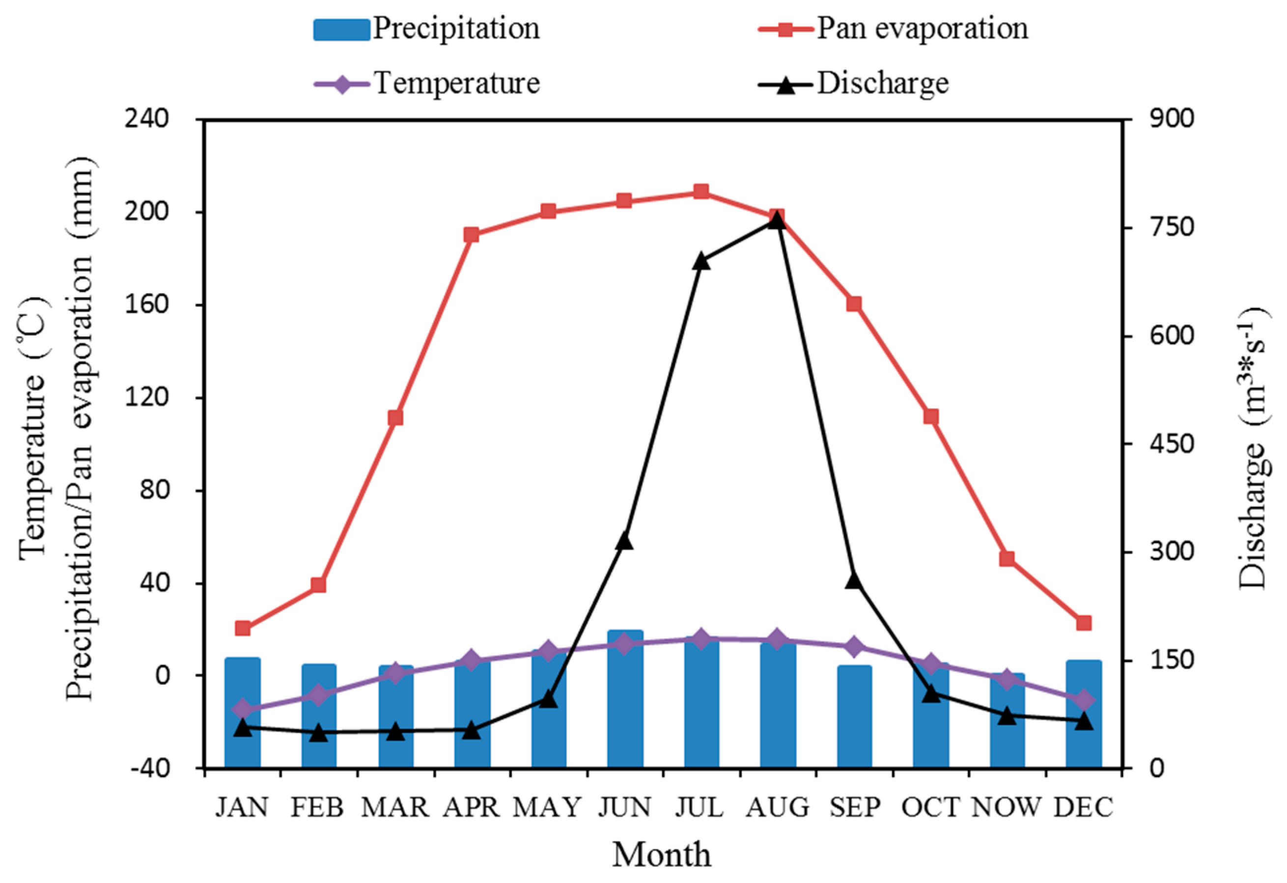
The Yarkant River basin (Figure 1) is located in Xinjiang Uygur Autonomous Region of China, and originates from the northern slope of Karakoram. The area of this catchment is 50,248 km2, and the elevation ranges from 8611 m to 1450 m with an average elevation of 4450 m. The climatic regime in this region is mostly controlled by the westerlies. There is only one meteorological station within the catchment area, Tashkurgan, which is located at 3090 m. At the Tashkurgan station, the annual precipitation, annual pan evaporation and mean annual temperature values are 96 mm, 1516 mm and 3.54 °C, respectively (Figure 2).
Snowpack and glaciers are mainly distributed above 5000 m and cover 26% of the whole catchment. The abundant snowpack and glaciers provide rich meltwater. At the catchment outlet of the Kaqun station (Figure 1), the average annual water volume is 6.87 × 10¹⁰ m3 (Figure 2). The water flux from June to September contributes 78.6% of the total annual discharge. These water resources support irrigation agriculture in the Yarkant River oasis, which is a major grain- and cotton-producing region in China and the largest agricultural irrigation region in Xinjiang, with an area of 2.5 × 10⁴ km2 [37]. This oasis is situated at the eastern edge of Taklimakan Desert; due to the harsh climate conditions, the ecological system is very vulnerable and strongly restricted by the water resources from the headstream of the Yarkant River. Consequently, under the influence of climate change, the availability of water resources for irrigated agriculture strongly affects the 2 million people living around the Yarkant River oasis.

2.2. Data

In this study, the Tashkurgan station’s daily observation data for 1986–2009 were obtained from the China Meteorological Data Sharing Service System (http://data.cma.cn/). These data include precipitation and mean/maximum/minimum temperature. The reference evapotranspiration was calculated using the Penman–Monteith equation and the formulation for reference crop evaporation [38]. Kaqun station’s daily discharge data for 2003–2009 were selected to calibrate (2003–2007) and validate (2008–2009) the hydrological model.
The daily precipitation and temperature outputs of 21 GCMs in Phase 5 of a Coupled Model Inter-comparison Project (CMIP5) [39] were selected as the sources of future meteorological data. The RCP4.5 and RCP8.5 scenarios were employed in this study. RCP4.5 is a stabilization scenario where the total radiative forcing is stabilized before 2100 through a range of technologies and strategies to reduce greenhouse gas emissions [40]. RCP8.5 is characterized by increasing greenhouse gas emissions over time and is representative of scenarios in the literature that lead to high concentration levels [41]. This paper categorizes the future CMIP5 model projections into four future periods (FPs) (2020–2039, FP1; 2040–2059, FP2; 2060–2079, FP3; and 2080–2099, FP4); 1986–2005 was selected as the historical period (HP).

3. Methodology

In relation to the HP, all change signals of precipitation and temperature in four FPs featured by each GCM were extracted statistically. Due to the uncertainty among GCMs, the average tendency of multiple GCMs was strongly suggested [32]; therefore, the average ensemble of available GCMs was employed. Based on the extracted change signals, the future precipitation and temperature in different periods, which were generated using a modified QPM and the Delta method, were used to force a well-calibrated MIKE SHE model. Then, the hydrological processes in future periods were obtained through MIKE SHE’s simulation. The modified QPM and the Delta method were used to analyse the data for each calendar month. The time series data of the GCMs’ historical and scenario runs were extracted for the location of Tashkurgan station (Figure 1).

3.1. Modified QPM for Precipitation

For the precipitation time series, the frequency change and quantile perturbation should not be completely independent indexes; rather, their relationship should be determined. In the modified QPM, the specific locations of added or subtracted rainfall events defined by frequency changes were determined in the ranked time series of precipitation data. Eleven quantiles, with values of 0.01, 0.05, 0.1, 0.2, 0.3, 0.4, 0.5, 0.6, 0.7, 0.8 and 0.9, were selected to divide the ranked time series into 12 segments in accordance with different grades of precipitation intensity. In each segment, the due number of rainy days can be calculated based on the quantile value and compared with the existing number of rainy days in this segment, and the added or subtracted number of rainy days can be determined.
A large deviation was noted in precipitation predicted by the GCM [24,42]. Therefore, to obtain a more accurate average trend from the selected GCMs, the annual precipitation given by 21 GCMs was used to check the consistency. The formulation was performed using Equation (1); the outliers identified by Equation (1) would be rejected by the consistency check.
P MEAN ± STD
where P is the annual precipitation of each GCM, and MEAN and STD are the average value and standard deviation of the 21 GCMs, respectively. According to the results of the consistency examination, three GCMs (CanESM2, ACCESS1.3 and HadGEM2-ES) were rejected. Based on the 18 remaining GCMs, the frequency change of rainy days when the daily precipitation exceeded 0.1 mm and the quantile perturbations at quantile i of each GCM were formulated as
f RD _ m = FP _ RD m HP _ RD m
f PI ( i , m ) = FP _ PI ( i , m ) HP _ PI ( i , m )
where f RD _ m is the monthly frequency change factor of rainy days in the mth month; FP _ RD m and HP _ RD m are the number of rainy days in the mth month of FPs and HP, respectively; f PI ( i , m ) is the precipitation intensity perturbation factor at quantile i in the mth month; and FP _ PI ( i , m )   and HP _ PI ( i , m ) are the precipitation intensities at quantile i in the mth month of FPs and HP, respectively. The average ensemble of the 18 GCMs is written as f RD _ m ¯ and f PI ( i , m ) ¯ .
For each calendar month (m = 1, 2, …, 11, 12), the detailed steps were as follows:
  • Calculate the number of rainy days ( OBS _ RD m ) and quantiles of each precipitation event ( OBS _ PI ( i , m ) ) in the observed time series of HP;
  • Interpolate FP _ PI ( i , m )   and HP _ PI ( i , m ) in the GCMs, maintaining the same quantile i with OBS _ PI ( i , m ) throughout the linear method, then calculate f PI ( i , m ) based on Equation (3) and f PI ( i , m ) ¯ ;
  • Obtain the future precipitation intensity at each quantile i ( NOBS _ PI ( i , m ) ), formulated as NOBS _ PI ( i , m ) = OBS _ PI ( i , m ) * f PI ( i , m ) ¯ ;
  • Obtain the number of future rainy days ( NOBS _ RD m ), formulated as NOBS _ RD m = OBS _ RD m * f RD _ m ¯ ;
  • Count the existing number of rainy days ( N E ) for which quantile i is not more than 0.01 in step 3;
  • Calculate the expected number of rainy days ( N D ) for which quantile i is not more than 0.01 based on the result in step 4, formulated as N D = NOBS _ RD m * 0.01. If N D > N E , ( N D N E ), no rainy days should be replaced in step 3, and the precipitation of added rainy days is equal to the average value of existing rainy days N E . Perform the above subtraction and round the difference between N D   and   N E to the nearest integer;
  • Sequentially repeat steps 5 and 6 at the other quantiles (0.05, 0.1, 0.2, 0.3, 0.4, 0.5, 0.6, 0.7, 0.8 and 0.9) until the number of rainy days in step 3 is equal to NOBS _ RD m .
In this modified QPM, a future precipitation time series that includes only the quantile perturbation signal is initially obtained in step 3. Then, through the frequency change in each segment divided by the quantiles, the lacking or redundant rainy days are defined (step 4 to step 6). Finally, by adding or subtracting these rainy days with fixed values in accordance to the precipitation intensity in each segment, the ranked time series of future precipitation data can be obtained.

3.2. Delta Method for Temperature

No frequency issues need to be considered for temperature; therefore, the Delta method [43,44] was employed to extract the monthly change signal of temperature. By calculating the monthly mean absolute difference between the HP and FPs in the GCMs, the change factor of temperature can be obtained. The future daily temperature was calculated as follows:
T NOBS ( m , d ) = T OBS ( m , d ) + ( T FP ( m ) T HP ( m ) )
where T NOBS ( m , d ) is the future temperatures of the FPs on the dth day in the mth month, T OBS ( m , d ) is the observation temperature on the dth day in the mth month, and T FP ( m ) and T HP ( m ) are the average temperatures predicted by the GCMs in mth month of four FPs and HP, respectively.

3.3. Hydrological Modelling

Because of the strong spatial heterogeneity due to the extreme topographical conditions, the fully distributed hydrological model MIKE SHE [45,46] was employed in this study to capture the detailed spatial variation. In the MIKE SHE model, the catchment is split into members of square grids, and the input data for each grid are input independently to describe the heterogeneity of the catchment. The relationships among the grids are linked via dynamic interactions. One-dimensional Richards Equation is used to calculate soil moisture distribution in unsaturated zone, and three-dimensional finite difference of the Darcy Equation is employed in the saturated zone. A simple day-degree method was employed in the MIKE SHE model to calculate snowmelt. Temperature values are typically the most readily available data and the most reliable as the primary factor in snow and ice melt simulation among hydrological simulations. Therefore, applications of the day-degree method are widespread and match the performance of the energy-balance method in the scarcely gauged region [47].
In the modelling of the Yarkant River basin, the MIKE SHE’s simulation resolution was 2 km and forcing data were obtained by interpolated observation. The simulation period ranged from 2000 to 2009, including the warm up period 2000–2002, the calibration period 2003–2007 and the validation period 2008–2009. The Auto Calibration Tool based on the global optimization algorithm Shuffled Complex Evolution (SCE) [48], which is part of the MIKE SHE package, was applied on a daily scale in this study. After sensitivity analysis based on a local sensitivity analysis method, the main significant parameters of snowmelt, including degree-day factor (DDF, range: 1–3 °C) and threshold melting temperature (TMT, range: −4–0 °C); land surface flow, including Manning values (MAN, range: 20–100 m1/3/s); interflow, including horizontal hydraulic conductivity (HHC, range: 1 × 10⁻⁶–5 × 10⁻³ m/s) and vertical hydraulic conductivity (VHC, range: 1 × 10⁻⁵–5 × 10⁻² m/s); and evapotranspiration, including leaf area index (LAI, range: 0–3) and root depth (RD, range: 0–4500 mm) were chosen for calibration. Considering the correlated parameters, it might be feasible to leave out one parameter in the calibration processes since no correct convergence point can be reached [49,50], correlation analysis was implemented, and results confirmed that there were no significant correlations between any two parameters under the significant level of 0.05. The optimized values of DDF and TMT were obtained using 2.01 mm/day/°C and −0.98 °C. MAN values ranged from 25 to 60 m1/3/s with respect to different land uses. HHC and VHC ranged from 0.0003 to 0.001 m/s and from 0.0035 to 0.01 m/s, respectively, across different soil types. More detailed information about the modelling and calibration can be found in our previous studies [51,52].
After calibration, at the Kaqun station (Figure 1), the Nash–Sutcliffe efficiency coefficients [53] were 0.71 and 0.66 between the observed and simulated daily discharge in the respective calibration and validation period, and the Pearson Correlation coefficients were 0.84 and 0.85, within the 95% confidence interval. This simulated flow hydrograph can be accepted. Additionally, our previous studies [51,52] have confirmed that the MIKE SHE model forcing by the interpolated station data obtained good simulation for many aspects of the hydrological processes. Therefore, the generated future meteorological data of the climate change signals can be used to force the well-calibrated MIKE SHE model to analyse the responses of the hydrological processes.

4. Results and Discussion

4.1. Future Climate Change

4.1.1. Precipitation

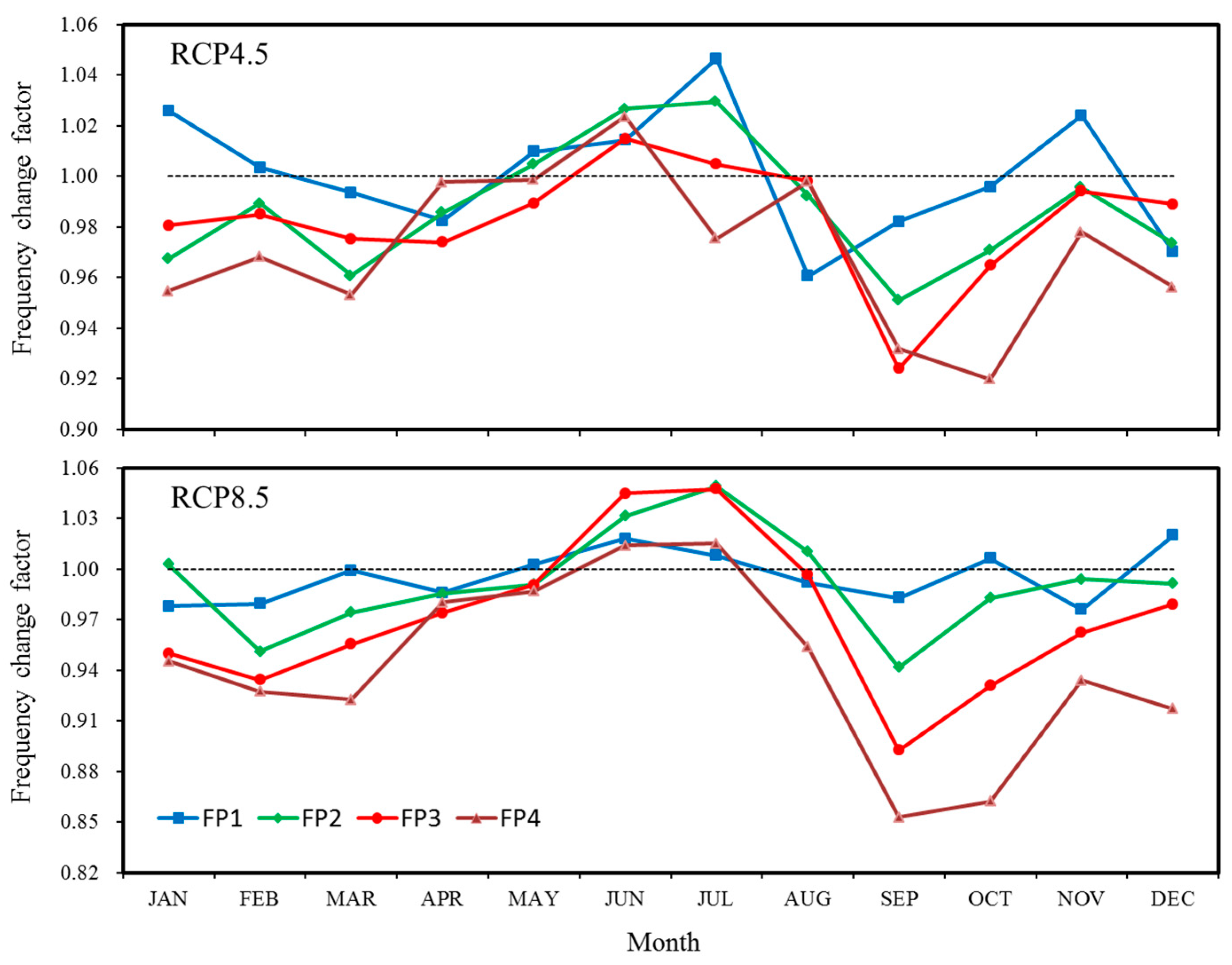
The mean monthly frequency changes determined by GCMs for the different FPs with respect to HP are similar between RCP4.5 and RCP8.5 (Figure 3). In general, from September to the following March, the number of rainy days continuously declines in FPs; this declining trend is stronger under RCP8.5 than under RCP4.5. Nevertheless, the number of rainy days generally increases in June and July and exhibits moderate change ratios. Regarding mean annual rainy days, 18 GCMs’ average ensemble indicates little change, with factors of 1.00, 0.99, 0.98 and 0.97 under RCP4.5 and of 1.00, 0.99, 0.97 and 0.94 under RCP8.5. However, the uncertainties among the 18 GCMs present large ranges: 0.92–1.09, 0.88–1.11, 0.90–1.11 and 0.88–1.11 under RCP4.5 and 0.93–1.07, 0.89–1.15, 0.84–1.18 and 0.76–1.04 under RCP8.5, and the deviations among 18 GCMs in the different periods mainly occur in summer.
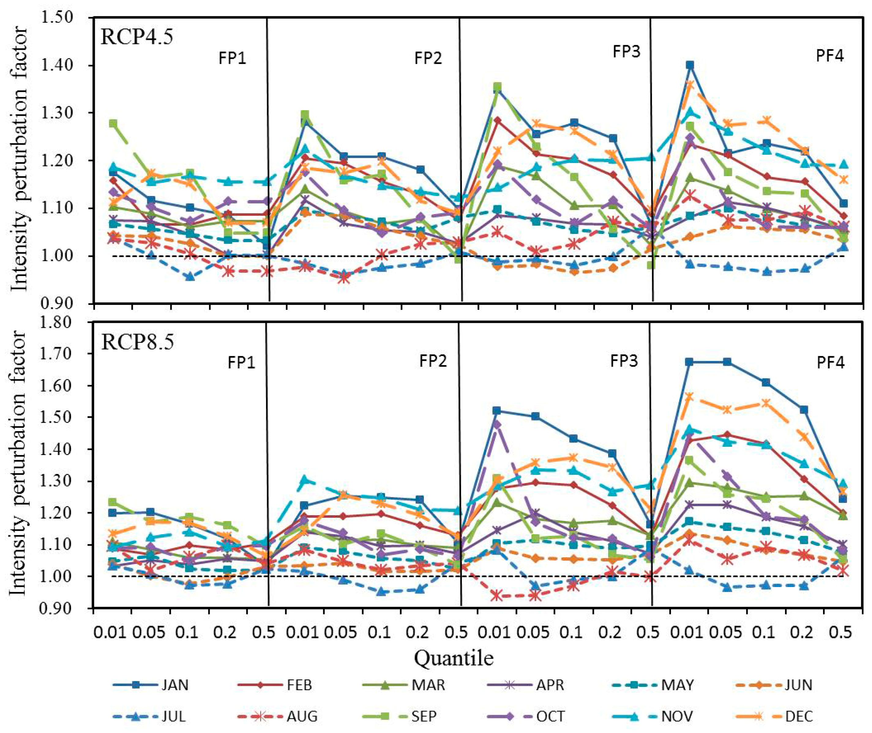
The precipitation data for the 0.01, 0.05, 0.1, 0.2 and 0.5 quantiles were chosen to illustrate the mean monthly quantile perturbations of precipitation intensity in the different FPs relative to those in HP determined by the GCMs (Figure 4). Under both scenarios, the rainfall intensities for the different quantiles do not drastically change in summer; however, the variations are quite significant in winter. The anabatic intensity of extreme precipitation (at the 0.01 quantile) in winter is the most significant; the aggravation is much stronger under RCP8.5 than under RCP4.5. For example, in January of FP4, the average increased proportion reaches 40% under RCP4.5 and 67% under RCP8.5, ranging from −19% to 221% under RCP4.5 and from −15% to 258% under RCP8.5. In contrast to the extreme precipitation, the other precipitation intensities show slightly increasing perturbations.
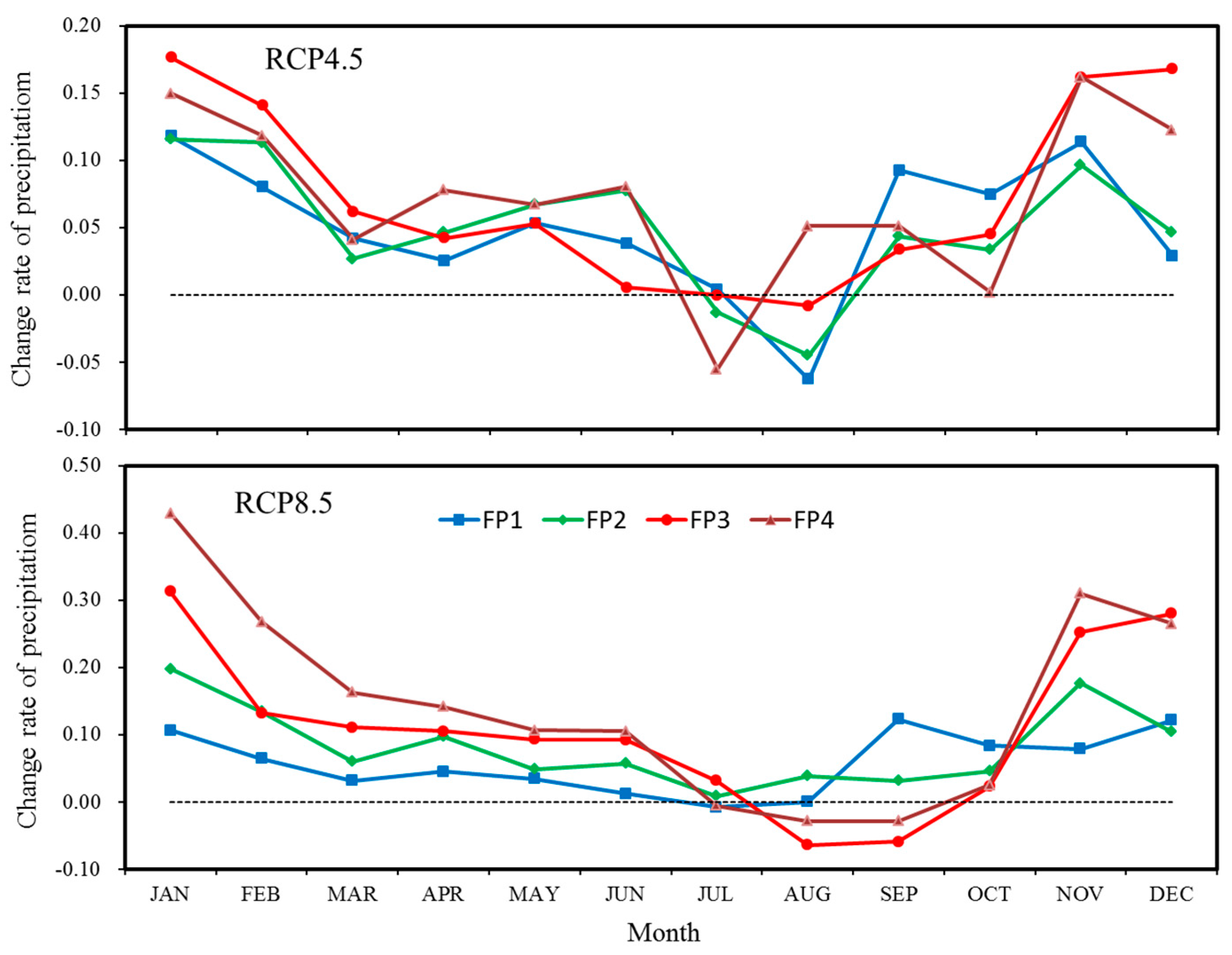
After adding the average change signals to the observations using the modified QPM, new time series were obtained to describe future situations. The monthly change rate of the precipitation volume in FPs is provided in Figure 5. Under both scenarios, owing to the incremental number of rainy days and reduced precipitation intensity, the precipitation volumes barely shift in summer. However, the stronger precipitation intensity is more than offset by the declining number of rainy days, and there is more abundant precipitation in winter. Compared with the annual precipitation in HP, FPs maintain upward tendencies of 2.9%, 3.6%, 3.0%, and 4.4% under RCP4.5, and 2.8%, 5.3%, 6.3%, and 7.9% under RCP8.5. Based on the average ensemble of 18 GCMs, in the future, primarily because of heavier extreme precipitation in winter, annual precipitation in the Yarkant River basin will exhibit a moderate increasing trend until 2100 under both scenarios, with a stronger trend under RCP8.5.

4.1.2. Temperature

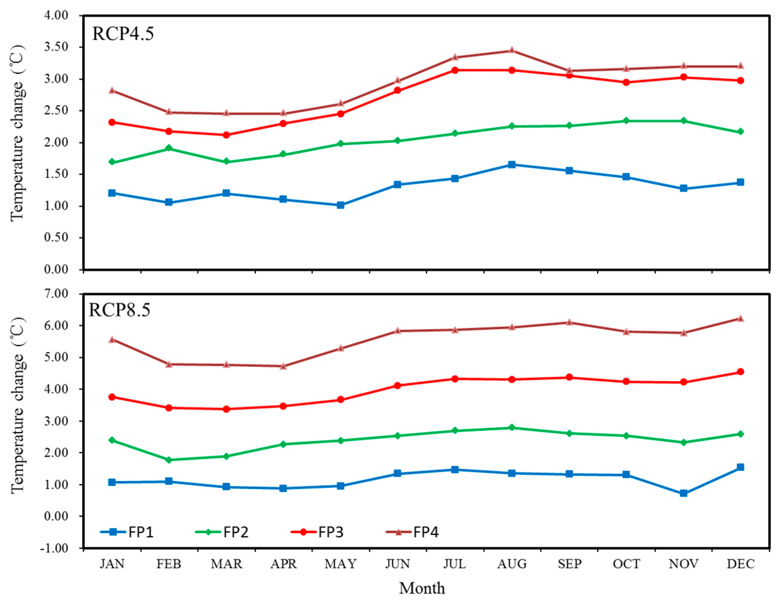
The monthly absolute change in temperature in FPs with respect to that of the HP is presented in Figure 6. Obviously, because of the different greenhouse gas emission scenarios, warming will slow at the end of this century under RCP4.5 but tend to continuously rise under RCP8.5. Compared with HP, the average increased rates predicted by the 18 GCMs for four FPs are 0.38 °C/10a, 0.38 °C/10a, 0.36 °C/10a and 0.31 °C/10a under RCP4.5, 0.34 °C/10a, 0.44 °C/10a, 0.53 °C/10a and 0.59 °C/10a under RCP8.5. The seasonal differences of warming are tiny. The 18 GCMs present a wide range of warming trends, e.g., in FP4, ranges of 0.17–0.75 °C/10a and 0.39–1.1 °C/10a are presented for two scenarios.
Considering the elevation-dependent warming in the mountain region [54], an additional nearby meteorological station, Pishan, which is at an elevation of 1375 m, was used to investigate the elevation lapse rate (EPR) of temperature in the GCMs. The average yearly temperatures predicted by the GCMs under both RCP4.5 and RCP8.5 at the Tashkurgan and Pishan stations are listed in Table 1. The warming trend in the lower-altitude region is stronger than that in the higher-altitude region under future climate change based on the EPR change in Table 1; therefore, the EPR of future temperature in the MIKE SHE model will decrease by 0.54 °C/km before 2060 and by 0.44 °C/km after 2060. It should be noted that the climate change trend in the low-altitude regions cannot be generalized to high-altitude regions. If elevation-dependent warming is not considered when processing temperature using GCMs, the warming in high-altitude regions will be overestimated and will result in large deviations. Such deviations will hinder our understanding of future changes in water resources.

4.2. Water Balance

Based on the simulated results for the Yarkant River basin produced using the MIKE SHE model, the quantified water balance components at the catchment scale are listed in Table 2 for each period. Because of the impact of climate change, all of the water components are correspondingly influenced. Clearly, the variations in dissipation (evapotranspiration) exceed those of stockpile (snow storage) and supply (streamflow to downstream), and the diminishing snow storage in the mountain region and decreasing streamflow supplied to the downstream region will be depleted through increasing evapotranspiration. These changes are more dramatic under RCP8.5 than under RCP4.5.

4.2.1. Snow

The accumulation and melting of snow are important processes in an alpine catchment’s hydrological cycle. Table 2 shows that mean annual snow storage will consistently diminish in the Yarkant River basin primarily because of the reduction in snowfall resulting from the rising temperature. The reductions will occur mainly in summer, from June to September. Based on the snowfall in HP, the change ratios of snowfall from June to September are −6.4~−28.9% under RCP4.5 and −3.4~−61.7% under RCP8.5. However, the change ratios in the remaining months are only −0.3~−6.8% under RCP4.5 and −0.9~−10.7% under RCP8.5. Thus, despite the warmer temperature, precipitation continues to rarely occur as rain in winter.
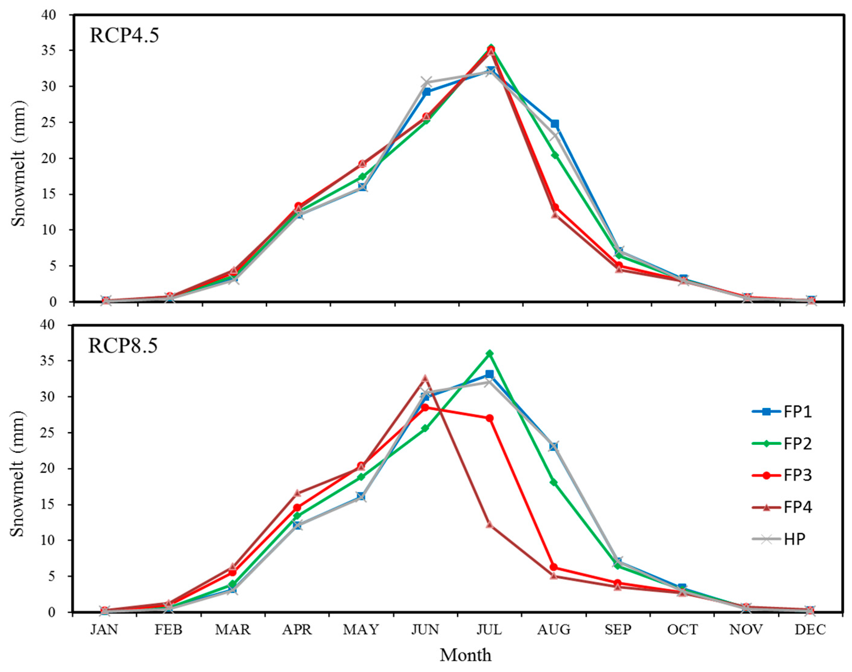
The monthly distribution of snowmelt in FP1 is similar to that in HP under both RCP4.5 and RCP8.5; however, after 2040, snowmelt increases in the earlier period (March to May) due to warming (Figure 7). This increased early snowmelt along with the drastically decreased snowfall in summer jointly result in less snow available for melting in the later period (August to October). This tendency will be more severe after 2060; after peaking in July, snowmelt will sharply decline under RCP4.5. Under RCP8.5, the peak in snowmelt is advanced to June, with little snowmelt in July and August.
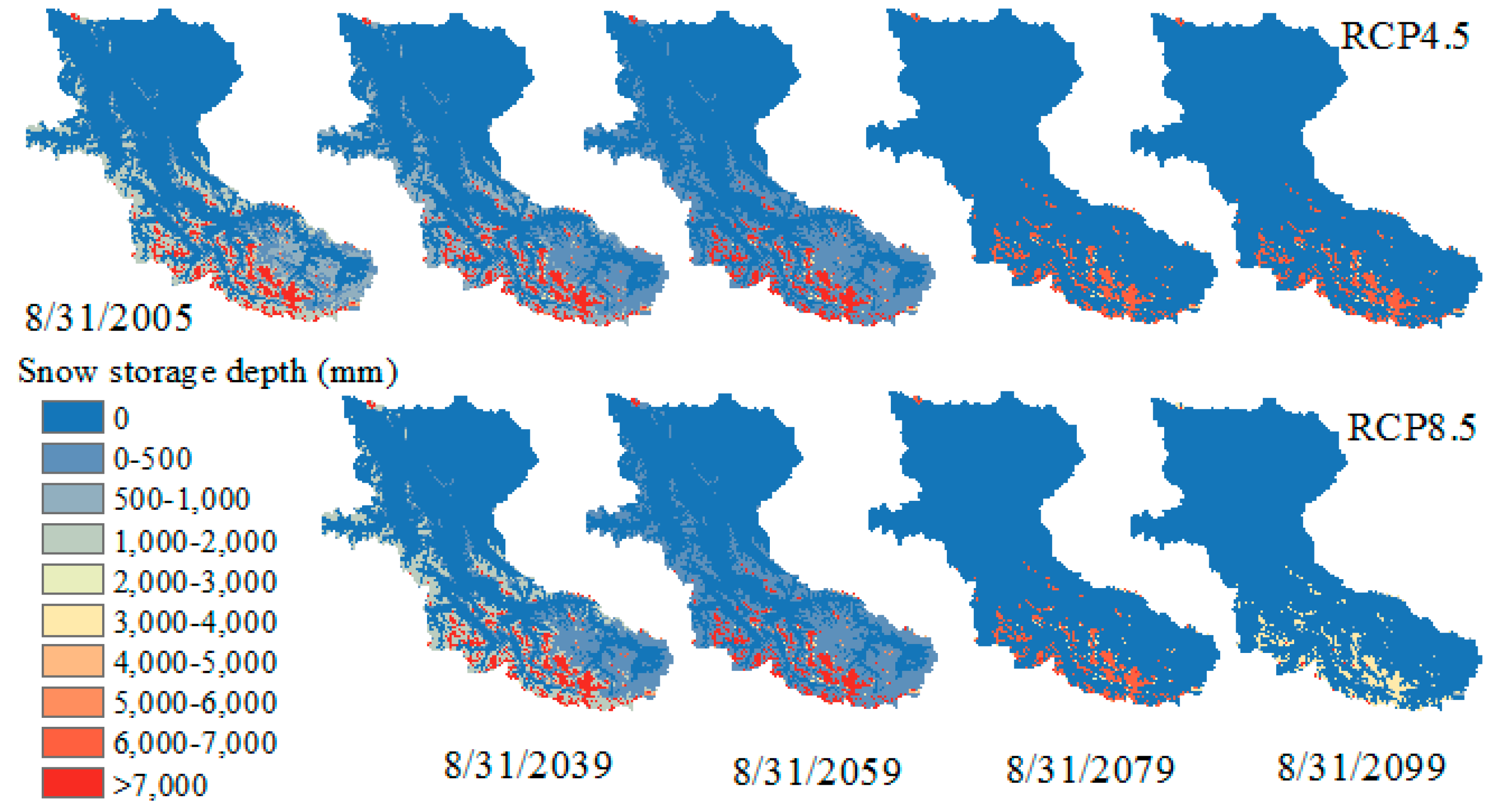
Regarding changes in snow storage, a new cycle of snowpack accumulation could begin in September; snow storage in August is the minimum of the entire year, so it is simply defined as permanent snow storage in this study. Figure 8 presents the spatial distribution of the snowpack on 31 August of the last year in each period. Under the RCP4.5 and RCP8.5 scenarios, before 2060, most of the middle mountain regions are covered by a thin snowpack, and the permanent snow cover area accounts for 34.4% of the entire catchment. However, the covered area in the middle mountain regions will vanish over the period 2060–2079, and the permanent snow storage area will occupy only 6% of the catchment.
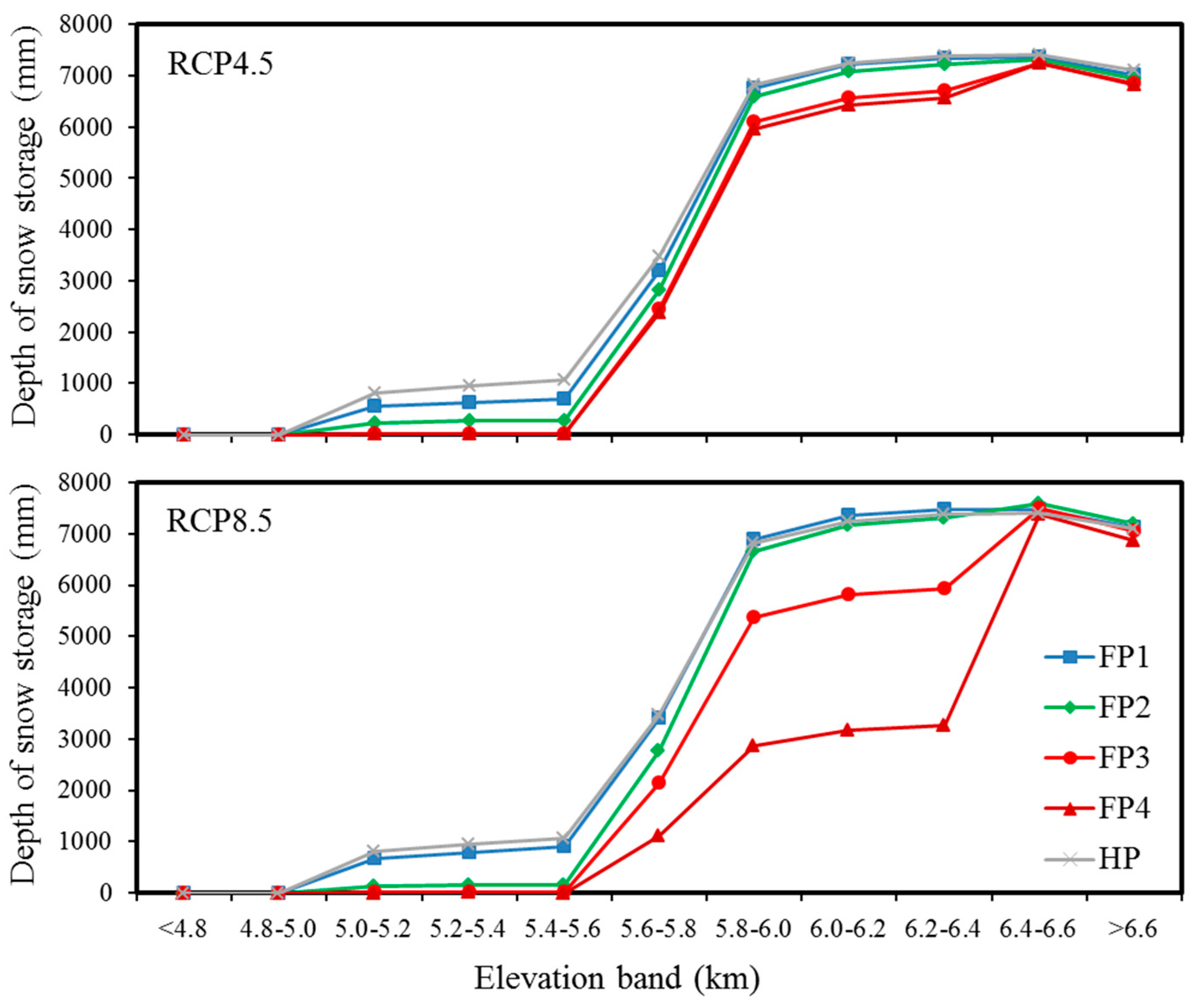
Figure 9 shows the distribution of permanent snow storage in different elevation bands. From before to after 2060, the coverage of permanent snow storage will rise by 600 m. Although the location of the permanent snow storage remains the same before 2060, the volumes of snow storage at 5000–5600 m in FP1 and FP2 will diminish significantly compared with the volumes in HP, i.e., by 33.2% and 72.1% under RCP4.5 and 16.4% and 84.4% under RCP8.5. The snow storage at 5600–6400 m could significantly shrink. The RCP4.5 climate change scenario indicates decreased snow storage at 5600–6400 m, i.e., 3.6–19.4% lower in FPs relative to HP. However, under RCP8.5, the effect is more acute: the percentages are reduced by 0.2–61% in four FPs. A different phenomenon occurs in the extremely cold region above 6400 m, where the average annual temperature was −19.5 °C in HP. The small or absent changes in permanent snow storage under both scenarios suggest that the rising temperature has little effect on the snow at this elevation because the increased temperature largely remains below the critical melting temperature of snow.

4.2.2. Streamflow

At the catchment outlet of the Kaqun station, streamflow in four FPs will change by −2.6%, −1.5%, −2.2%, and −3.5% under RCP4.5 and −3.7%, 1.7%, −2.2%, and −6.0% under RCP8.5 (Table 2) relative to HP. In general, runoff shows a decreasing tendency, which suggests that less water resources will be available for downstream regions. Similar to snowmelt, streamflow increases in spring and early summer and decreases in late summer (Figure 10). In FP1, the monthly stream flow at Kaqun maintains a very similar distribution to that in HP; however, in FP2, the discharge in May and July begins to rise because of the increased amount of melt water. Furthermore, in FP3 and FP4, the reductions of streamflow in August and September are also significant. All of these changes are strongly correlated with the changes in snowmelt. From a temporal perspective, May to September will remain as the flood season, with contribution ratios of 80.5–82.8% under RCP4.5 and 80.6–83.6% under RCP8.5. This very moderate growth discharge in the flood season is mainly ascribed to stronger, more frequent flood events and can be further explained by the following analysis.
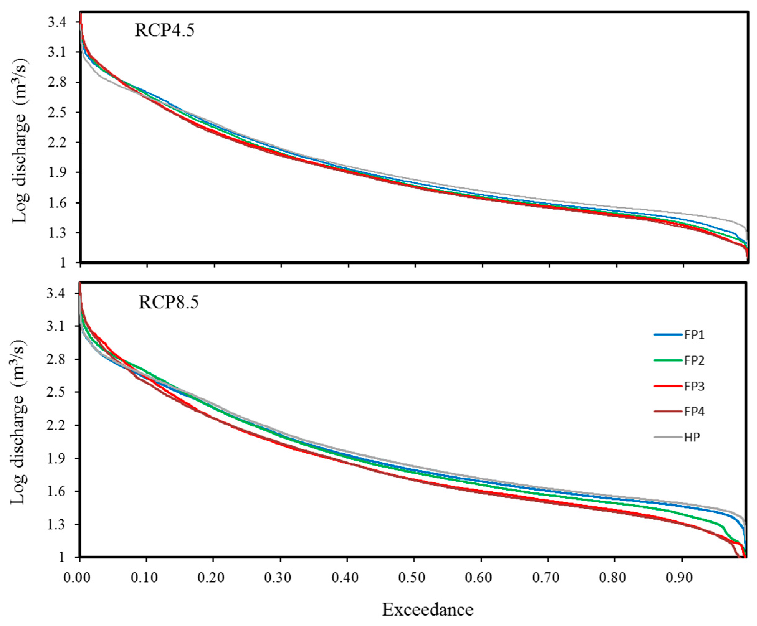
Figure 11 illustrates the exceedance probability curves of the simulated discharge at the Kaqun station for each period. For extreme flows with exceedance probabilities below 0.08, the average discharge increases by 17.2–25.6% in four FPs relative to HP under RCP4.5; the corresponding values for RCP8.5 are 1.4–20.6%. Small flows with exceedance probabilities above 0.4 are correspondingly reduced by 8.6–18.3% under RCP4.5 and by 6.4–27.0% under RCP 8.5. The variance of the flow probability indicates that the disequilibrium of the water resource will be more severe in the future; thus, more water will be involved in flood events, and less water will be available in the dry season. These phenomena are stronger under RCP8.5 than under RCP4.5. One possible reason for these changes is that more snowfall will be replaced by rainfall, and more meltwater will be produced in early summer. These variations will accelerate river conflux and increase the frequency and intensity of flooding. For instance, for a daily discharge above 1000 m3/s (with exceedance probabilities less than 0.01), the occurrence frequencies are 1.8–2.5% in FPs of RCP4.5 and 1.1–2.3% in those of RCP8.5. However, the occurrence value is only 1% in HP. Additionally, the occurrence time is advanced from the middle of June in HP to early June after 2020 and as early as late May after 2060.

5. Conclusions

A 21-member average ensemble of GCMs under RCP4.5 and RCP8.5 was used to analyse the impacts of climate change on the Yarkant River basin in Karakoram. A modified QPM was employed to extract the change signals of precipitation in the GCMs. In this modified QPM, according to the frequency variations in different quantile segments, added and subtracted rainy days were assigned to a fixed range in the ranked time series. The Delta method with elevation-dependent warming was applied to process the temperature change trends in the GCMs. All of the change signals of precipitation and temperature presented notable uncertainties among the employed GCMs. Referring to the observed meteorological data in the baseline period, an average ensemble of change signals was used to generate future meteorological data. Combined with a well-calibrated MIKE SHE model, the responses of hydrological processes to climate change were analysed from a water balance perspective.
In the Yarkant River basin, the increase in precipitation in four FPs (mean ratios of 2.9–4.4% under RCP4.5 and 2.8–7.9% under RCP8.5) in this century will be primarily triggered by the enhanced intensity of extreme precipitation in winter. Under both scenarios, the slight increase in the frequency of precipitation and the decrease in the intensity of precipitation at different quantiles result in little variation in precipitation volume in summer. In winter, the stronger precipitation intensity is more than offset by the decline in the number of rainy days, and consequently, the precipitation in winter exhibits an increasing trend. For temperature, the warming tendencies are obviously distinct between the two scenarios: RCP4.5 shows moderate mean ratios ranging from 0.31/10a to 0.38/10a in four FPs, but RCP8.5 presents ever-increasing values ranging from 0.34/10a to 0.59/10a. Furthermore, because warming is elevation dependent, the temperature in the low-altitude region increases more dramatically than that in the high-altitude region, and the EPR values indicate differences of 0.54 °C/km and 0.44 °C/km before and after 2060, respectively.
Under the influence of climate change, the spatiotemporal distribution of snow will be sharply altered, and large variation will develop among the different elevation bands. In each FP, snowfall will decrease significantly from June to September, i.e., by 6.4–28.9% under RCP4.5 and by 3.4–61.7% under RCP8.5, and the snowmelt from March to May will be enhanced. As a result, increasingly less snowpack is available for melting from August to October. With respect to the permanently snow-covered region, the altitude will rise by 600 m over the period 2060–2079, and all of the covered area at 5000–5600 m will completely vanish. At 5600–6400 m, snow storage will diminish significantly (by 19.4% under RCP4.5 and 61% under RCP8.5) by the end of this century. However, above 6400 m, because increased temperatures rarely exceed the critical value for snowmelt, little or no change in snow storage will occur in this region.
The streamflow at the catchment outlet will exhibit a moderate decreasing trend and more severe disequilibrium. Because of the more intense dissipation via evapotranspiration, the predicted discharge in FPs at Kaqun station will diminish by 1.5–3.5% under RCP4.5 and 2.2–6% under RCP8.5. More importantly, the runoff distribution will be much more incongruous. As the snowmelt changes, the streamflow will increase from spring until early summer and decrease in late summer. Furthermore, earlier and stronger flood events will occur more frequently.
In the Yarkant River basin, future climate change will strongly impact hydrological processes and trigger a significant reforming of water resources. The evapotranspiration dissipation of water resources will be enhanced. The reductions in the snow-covered area and snow storage volume will reduce water storage in solid form in the high mountain region. Declining streamflow at the mountain outlet will threaten the amount of available water resources for agricultural irrigation downstream. Moreover, in future flood periods, greater flood discharge and more frequent flood events will create greater challenges for flood security. These responses of hydrological processes indicate that future climate change could strongly affect water resources and that a new strategy for irrigation agriculture in the downstream region is needed in order to adapt to the variation in the water supplied by the alpine catchment.

Acknowledgments

We gratefully thank the Tarim Water Resources Management Bureau for providing the necessary data. This work was financially supported by International Partnership Program of the Chinese Academy of Sciences (131551KYSB20160002), One Thousand Youth Talents Plan of China (Xinjiang Project: Y374231), the Project of Chinese Academy of Sciences (Y674122, Y634261), and Natural Sciences Foundation of China (U1503183).

Author Contributions

Jiao Liu conducted the major data processing and modelling works and wrote manuscript. Min Luo supported the GCM and processed the simulated results. Tie Liu designed part of the MIKE SHE model and analyzed the simulated results. Anming Bao decided the data choosing and made some interpretations of results. Phillipe De Maeyer revised the manuscript’s structure and language and contributed to its professionalism. Xianwei Feng revised the language editing and contributed the structure of this paper. Xi Chen evaluated and suggested the manuscript with respect to the study’s goals.

Conflicts of Interest

The authors declare no conflict of interest.

References

  1. IPCC. Climate Change 2013: The Physical Science Basis. Contribution of Working Group I to the Fifth Assessment Report of IPCC; Cambridge University Press: Cambridge, UK; New York, USA, 2013. [Google Scholar] [CrossRef]
  2. Chen, Y.; Takeuchi, K.; Xu, C.; Chen, Y.; Xu, Z. Regional climate change and its effects on river runoff in the Tarim basin, China. Hydrol. Process. 2006, 20, 2207–2216. [Google Scholar] [CrossRef]
  3. Guo, L.; Li, L. Variation of the proportion of precipitation occurring as snow in the Tian Shan mountains, China. Int. J. Climatol. 2015, 35, 1379–1393. [Google Scholar] [CrossRef]
  4. Huss, M.; Farinotti, D.; Bauder, A.; Funk, M. Modelling runoff from highly glacierized alpine drainage basins in a changing climate. Hydrol. Process. 2008, 22, 3888–3902. [Google Scholar] [CrossRef]
  5. Springer, C.; Matulla, C.; Schöner, W.; Steinacker, R.; Wagner, S. Downscaled GCM projections of winter and summer mass balance for Central European glaciers (2000–2100) from ensemble simulations with ECHAM5-MPIOM. Int. J. Climatol. 2013, 33, 1270–1279. [Google Scholar] [CrossRef]
  6. Barontini, S.; Grossi, G.; Kouwen, N.; Maran, S.; Scaroni, P.; Ranzi, R. Impacts of climate change scenarios on runoff regimes in the southern Alps. Hydrol. Earth Syst. Sci. 2009, 6, 3089–3141. [Google Scholar] [CrossRef]
  7. Liu, S.Y.; Yong, Z.; Song, Z.Y.; Yong, D. Estimation of glacier runoff and future trends in the Yangtze River source region, China. J. Glaciol. 2009, 55, 353–362. [Google Scholar] [CrossRef]
  8. Jeelani, G.; Feddema, J.J.; Veen, C.J.; Stearns, L. Role of snow and glacier melt in controlling river hydrology in Liddar watershed (western Himalaya) under current and future climate. Water Resour. Res. 2012, 48, 12508. [Google Scholar] [CrossRef]
  9. Bavay, M.; Grünewald, T.; Lehning, M. Response of snow cover and runoff to climate change in high Alpine catchments of eastern Switzerland. Adv. Water Resour. 2013, 55, 4–16. [Google Scholar] [CrossRef]
  10. Su, F.; Zhang, L.; Ou, T.; Chen, D.; Yao, T.; Tong, K.; Qi, Y. Hydrological response to future climate changes for the major upstream river basins in the Tibetan Plateau. Glob. Planet. Chang. 2016, 136, 82–95. [Google Scholar] [CrossRef]
  11. Immerzeel, W.W.; van Beek, L.P.; Bierkens, M.F. Climate change will affect the Asian water towers. Science 2010, 328, 1382–1385. [Google Scholar] [CrossRef] [PubMed]
  12. Calanca, P.; Roesch, A.; Jasper, K.; Wild, M. Global warming and the summertime evapotranspiration regime of the Alpine region. Clim. Chang. 2006, 79, 65–78. [Google Scholar] [CrossRef]
  13. Thompson, J.R.; Green, A.J.; Kingston, D.G. Potential evapotranspiration-related uncertainty in climate change impacts on river flow: An assessment for the Mekong River basin. J. Hydrol. 2014, 510, 259–279. [Google Scholar] [CrossRef]
  14. Roosmalen, L.V.; Sonnenborg, T.O.; Jensen, K.H. Impact of climate and land use change on the hydrology of a large-scale agricultural catchment. Water Resour. Res. 2009, 45, 150–164. [Google Scholar] [CrossRef]
  15. Chen, Y.; Xu, C.; Chen, Y.; Li, W.; Liu, J. Response of glacial-lake outburst floods to climate change in the Yarkant River basin on northern slope of Karakoram mountains, China. Quat. Int. 2010, 226, 75–81. [Google Scholar] [CrossRef]
  16. Xu, H.; Zhou, B.; Song, Y. Impacts of climate change on headstream runoff in the Tarim River Basin. Hydrol. Res. 2010, 42, 20–29. [Google Scholar] [CrossRef]
  17. Zhang, Q.; Xu, C.Y.; Tao, H.; Jiang, T.; Chen, Y.D. Climate changes and their impacts on water resources in the arid regions: A case study of the Tarim River basin, China. Stoch. Environ. Res. Risk Assess. 2010, 24, 349–358. [Google Scholar] [CrossRef]
  18. Xu, C.; Chen, Y.; Chen, Y.; Zhao, R.; Ding, H. Responses of surface runoff to climate change and human activities in the arid region of central Asia: A case study in the Tarim River basin, China. Environ. Manag. 2013, 51, 926–938. [Google Scholar] [CrossRef] [PubMed]
  19. Zhang, S.; Gao, X.; Zhang, X.; Hagemann, S. Projection of glacier runoff in Yarkant River basin and Beida River basin, Western China. Hydrol. Process. 2012, 26, 2773–2781. [Google Scholar] [CrossRef]
  20. Onyutha, C.; Tabari, H.; Rutkowska, A.; Nyeko-Ogiramoi, P.; Willems, P. Comparison of different statistical downscaling methods for climate change rainfall projections over the Lake Victoria basin considering CMIP3 and CMIP5. J. Hydrol. Environ. Res. 2016, 12, 31–45. [Google Scholar] [CrossRef]
  21. Min, S.K.; Zhang, X.; Zwiers, F.W.; Hegerl, G.C. Human contribution to more-intense precipitation extremes. Nature 2011, 470, 378–381. [Google Scholar] [CrossRef] [PubMed]
  22. Salathé, E.P.; Hamlet, A.F.; Mass, C.F.; Lee, S.; Stumbaugh, M.; Steed, R. Estimates of twenty-first-century flood risk in the Pacific Northwest based on regional climate model simulations. J. Hydrometeorol. 2014, 15, 1881–1899. [Google Scholar] [CrossRef]
  23. Quintana Seguí, P.; Ribes, A.; Martin, E.; Habets, F.; Boé, J. Comparison of three downscaling methods in simulating the impact of climate change on the hydrology of Mediterranean basins. J. Hydrol. 2010, 383, 111–124. [Google Scholar] [CrossRef]
  24. Liu, T.; Willems, P.; Pan, X.L.; Bao, A.M.; Chen, X.; Veroustraete, F.; Dong, Q.H. Climate change impact on water resource extremes in a headwater region of the Tarim basin in China. Hydrol. Earth Syst. Sci. 2011, 15, 3511–3527. [Google Scholar] [CrossRef]
  25. Taye, M.T.; Ntegeka, V.; Ogiramoi, N.P.; Willems, P. Assessment of climate change impact on hydrological extremes in two source regions of the Nile River Basin. Hydrol. Earth Syst. Sci. 2011, 15, 209–222. [Google Scholar] [CrossRef]
  26. Willems, P.; Vrac, M. Statistical precipitation downscaling for small-scale hydrological impact investigations of climate change. J. Hydrol. 2011, 402, 193–205. [Google Scholar] [CrossRef]
  27. Ntegeka, V.; Baguis, P.; Roulin, E.; Willems, P. Developing tailored climate change scenarios for hydrological impact assessments. J. Hydrol. 2014, 508, 307–321. [Google Scholar] [CrossRef]
  28. Lettenmaier, D.P.; Wood, A.W.; Palmer, R.N.; Wood, E.F.; Stakhiv, E.Z. Water resources implications of global warming: A U.S regional perspective. Clim. Chang. 1999, 43, 537–579. [Google Scholar] [CrossRef]
  29. Middelkoop, H.; Daamen, K.; Gellens, D.; Grabs, W.; Kwadijk, J.C.; Lang, H.; Parment, B.A.; Schadler, B.; Schulla, J.; Wilke, K. Impact of ClimateChange on the Hydrological Regime and Water Resources Management in the Rhine Basin. Clim. Chang. 2001, 49, 105–128. [Google Scholar] [CrossRef]
  30. Ntegeka, V.; Willems, P.; Baguis, P.; Roulin, E. Climate Change Impact on Hydrological Extremes along Rivers and Urban Drainage Systems in Belgium; Summary Report Phase 1: Literature Review and Development of Climate Change Scenarios: Belgian Science Policy-SSD Research Programme, CCI-HYDR Project; KU Leuven: Leuven/Brussels, Belgium, 2008. [Google Scholar]
  31. Chen, J.; Brissette, F.P.; Leconte, R. Uncertainty of downscaling method in quantifying the impact of climate change on hydrology. J. Hydrol. 2011, 401, 190–202. [Google Scholar] [CrossRef]
  32. Ghosh, S.; Katkar, S. Modeling uncertainty resulting from multiple downscaling methods in assessing hydrological impacts of climate change. Water Resour. Manag. 2012, 26, 3559–3579. [Google Scholar] [CrossRef]
  33. Teng, J.; Vaze, J.; Chiew, F.H.S.; Wang, B.; Perraud, J. Estimating the relative uncertainties sourced from GCMs and hydrological models in modeling climate change impact on runoff. J. Hydrometeorol. 2012, 13, 122–139. [Google Scholar] [CrossRef]
  34. Foley, A.M. Uncertainty in regional climate modelling: A review. Prog. Phys. Geogr. 2010, 34, 647–670. [Google Scholar] [CrossRef]
  35. Refsgaard, J.C.; Sonnenborg, T.; Butts, M.; Christensen, J.H.; Christensen, S.; Drews, M.; Jensen, K.H.; Jørgensen, F.; Larsen, M.; Rasmussen, S.; et al. Climate change impacts on groundwater hydrology—Where are the main uncertainties and can they be reduced? Hydrol. Sci. J. 2016, 61, 2312–2324. [Google Scholar] [CrossRef]
  36. Refsgaard, J.C.; Christensen, S.; Sonnenborg, T.; Seifert, D.; Højberg, A.L.; Troldborg, L. Review of strategies for handling geological uncertainty in groundwater flow and transport modeling. Adv. Water Resour. 2012, 36, 36–50. [Google Scholar] [CrossRef]
  37. Hong, T.; Gang, Y.D.; Fang, Z.Y. Food security and agricultural structural adjustment in Yarkant River Basin, northwest China. Journal of Food. Agric. Environ. 2013, 11, 324–328. [Google Scholar]
  38. Allen, R.G.; Pereira, L.S.; Raes, D.; Smith, M. Crop Evapotranspiration-Guidelines for Computing Crop Water Requirements—FAO Irrigation and Drainage Paper 56; F.A.O.: Rome, Italy, 1998; ISBN 92-5-104219-5. [Google Scholar]
  39. Taylor, K.E.; Stouffer, R.J.; Meehl, G.A. An overview of CMIP5 and the experiment design. Am. Meteorol. Soc. 2012, 93, 485–498. [Google Scholar] [CrossRef]
  40. Clarke, L.; Edmonds, J.; Jacoby, H.; Pitcher, J.; Reilly, J.; Richels, R. Scenarios of Greenhouse Gas Emissions and Atmospheric Concentrations; Sub-Report 2.1A of Synthesis and Assessment Product 2.1 by the U.S. Climate Change Science Program and the Subcommittee on Global Change Research; Office of Biological & Environmental Research, Department of Energy: Washington, DC, USA, 2007; p. 154.
  41. Riahi, K.; Gruebler, A.; Nakicenovic, N. Scenarios of long-term socio-economic and enviromental development under climate stabilization. Technol. Forecast. Soc. Chang. 2007, 74, 887–935. [Google Scholar] [CrossRef]
  42. Baguis, P.; Roulin, E.; Willems, P.; Ntegeka, V. Climate change scenarios for precipitation and potential evapotranspiration over central Belgium. Theor. Appl. Climatol. 2010, 99, 273–286. [Google Scholar] [CrossRef]
  43. Gleick, P.H. Methods for evaluating the regional hydrologic impacts of global climatic changes. J. Hydrol. 1986, 88, 97–116. [Google Scholar] [CrossRef]
  44. Hay, L.E.; Wilby, R.L.; Leavesley, G.H. A comparison of delta change and downscaled GCM scenarios for three mountainous basins in the United States. J. Am. Water Resour. Assoc. 2000, 36, 387–397. [Google Scholar] [CrossRef]
  45. Abbott, M.B.; Bathurst, J.C.; Cunge, J.A.; O’connell, P.E.; Rasmussen, J. An introduction to the European Hydrological System—Systeme Hydrologique Europeen, “SHE”, 2: Structure of a physically-based, distributed modelling system. J. Hydrol. 1986, 87, 61–77. [Google Scholar] [CrossRef]
  46. Graham, D.; Butts, M. Chapter 10: Flexible integrated watershed modeling with MIKE SHE. In Watershed Models; Singh, V., Frevert, D., Eds.; CRC Press: Boca Raton, FL, USA, 2005; pp. 245–272. ISBN 0849336090. [Google Scholar]
  47. Hock, R. Glacier melt: A review of processes and their modelling. Prog. Phys. Geogr. 2005, 29, 362–391. [Google Scholar] [CrossRef]
  48. Vrugt, J.A.; Gupta, H.V.; Bouten, W.; Sorooshian, S. A shuffled complex evolution Metropolis algorithm for optimization and uncertainty assessment of hydrologic model parameters. Water Resour. Res. 2003, 39, 113–117. [Google Scholar] [CrossRef]
  49. Refsgaard, J.C. Parameterisation, calibration and validation of distributed hydrological models. J. Hydrol. 1997, 198, 69–97. [Google Scholar] [CrossRef]
  50. Hill, M.C. Methods and Guidelines for Effective Model Calibration; Water Resources Investigations Resport; U.S. Geological Survey: Denver, CO, USA, 1998; pp. 24–29.
  51. Liu, J.; Liu, T.; Bao, A.; De Maeyer, P.; Kurban, A.; Chen, X. Response of hydrological processes to input data in high alpine catchment: An assessment of Yarkant River in China. Water 2016, 8, 181. [Google Scholar] [CrossRef]
  52. Liu, J.; Liu, T.; Bao, A.; De Maeyer, P.; Feng, X.W.; Miller, S.N.; Chen, X. Assessment of different modelling studies on the spatial hydrological processes in an arid Alpine catchment. Water Resour. Manag. 2016, 30, 1757–1770. [Google Scholar] [CrossRef]
  53. Nash, J.E.; Sutcliffe, J.V. River flow forecasting through conceptual models part I—A discussion of principles. J. Hydrol. 1970, 10, 282–290. [Google Scholar] [CrossRef]
  54. Rangwala, I.; Miller, J.R. Climate change in mountains: A review of elevation-dependent warming and its possible causes. Clim. Chang. 2012, 114, 527–547. [Google Scholar] [CrossRef]
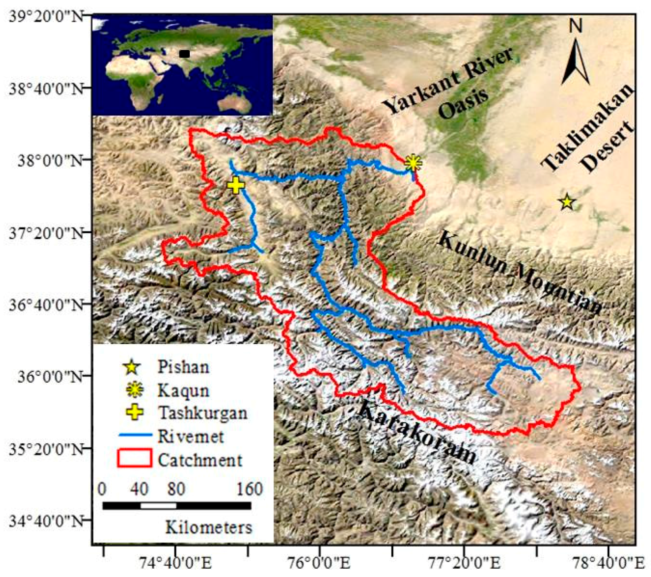
Figure 1. The locations of the Yarkant River basin, meteorological and hydrological stations.
Water 09 00344 g001
Figure 2. Monthly precipitation, pan evaporation and temperature values at the Tashkurgan station and discharge at the Kaqun station.
Water 09 00344 g002
Figure 3. The mean frequency changes of the rainy days in each month of the future periods (FPs) relative to those of the history period (HP) determined by the 18 Global Circulation Models (GCMs).
Water 09 00344 g003
Figure 4. The mean quantile perturbations of the precipitation intensity in each month of the future periods (FPs) relative to those of the history period (HP) determined by the 18 GCMs.
Water 09 00344 g004
Figure 5. The amount of monthly precipitation change rates generated in the future periods (FPs) with respect to those observed in the history period (HP).
Water 09 00344 g005
Figure 6. The mean monthly changes of temperature of the future periods (FPs) compared to those of the history period (HP) determined by the 18 GCMs.
Water 09 00344 g006
Figure 7. The amount of monthly snowmelt simulated by the MIKE SHE model in the history period (HP) and future periods (FPs).
Water 09 00344 g007
Figure 8. The spatial distribution of the snowpack simulated by the MIKE SHE model on 31 August of the last year in each period.
Water 09 00344 g008
Figure 9. The distributions of permanent snow storage simulated by the MIKE SHE model in the different elevation bands of the catchment on 31 August of the last year in each period.
Water 09 00344 g009
Figure 10. Average monthly discharge simulated by the MIKE SHE model in each period at the Kaqun station.
Water 09 00344 g010
Figure 11. Exceedance probabilities of the simulated discharge simulated by the MIKE SHE model at the Kaqun station in each period.
Water 09 00344 g011
Table 1. The average yearly temperatures determined by the GCMs (RCP4.5/RCP8.5) at the Tashkurgan and Pishan stations and the elevation lapse rates (EPR) in GCM calculated based on these two stations.
PeriodHPFP1FP2FP3FP4
Tashkurgan (°C)−5.84−4.53/−4.68−3.79/−3.46−3.13/−1.84−2.90/−0.29
Pishan (°C)3.2165.45/5.36.18/6.496.69/7.956.90/9.5
EPR (°C/km)−5.28−5.82/−5.82−5.81/−5.8−5.73/−5.71−5.72/−5.71
Table 2. The annual amounts of the water balance components (RCP4.5/RCP8.5) simulated by the MIKE SHE model in the Yarkant River basin during each period.
PeriodHPFP1FP2FP3FP4
Precipitation (mm)262.1269.8/268.4268.8/274.5270.0/278.0273.7/279.4
Snowfall (mm)165.1161.1/165.1151.1/150.7141.0/129.2138.7/112.2
Snow storage (mm)36.931.8/34.625.5/23.920.7/18.120.3/10.6
Stream runoff (mm)110.2107.5/106.1108.5/112.1107.7/107.8106.3/103.6
Evapotranspiration (mm)108.6118.3/119.9123.7/129.5128.7/143.1132.1/155.9