Article

Daily Based Morgan–Morgan–Finney (DMMF) Model: A Spatially Distributed Conceptual Soil Erosion Model to Simulate Complex Soil Surface Configurations

1
Biogeographical Modelling, Bayreuth Center of Ecology and Environmental Research (BayCEER), University of Bayreuth, Universitätsstraße 30, D-95440 Bayreuth, Germany
2
Professorship of Ecological Services, Faculty of Biology, Chemistry and Earth Sciences, BayCEER, University of Bayreuth, Universitätsstraße 30, D-95440, Bayreuth, Germany
3
Soil Physics Group, University of Bayreuth, Universitätstraße 30, D-95440 Bayreuth, Germany
4
Univ. Grenoble Alpes, Irstea, EMGR, F-38000 Grenoble, France
*
Author to whom correspondence should be addressed.
Water 2017, 9(4), 278; https://doi.org/10.3390/w9040278
Submission received: 24 February 2017 / Revised: 10 April 2017 / Accepted: 11 April 2017 / Published: 17 April 2017
(This article belongs to the Special Issue Soil Erosion by Water)

Abstract

:
In this paper, we present the Daily based Morgan–Morgan–Finney model. The main processes in this model are based on the Morgan–Morgan–Finney soil erosion model, and it is suitable for estimating surface runoff and sediment redistribution patterns in seasonal climate regions with complex surface configurations. We achieved temporal flexibility by utilizing daily time steps, which is suitable for regions with concentrated seasonal rainfall. We introduce the proportion of impervious surface cover as a parameter to reflect its impacts on soil erosion through blocking water infiltration and protecting the soil from detachment. Also, several equations and sequences of sub-processes are modified from the previous model to better represent physical processes. From the sensitivity analysis using the Sobol’ method, the DMMF model shows the rational response to the input parameters which is consistent with the result from the previous versions. To evaluate the model performance, we applied the model to two potato fields in South Korea that had complex surface configurations using plastic covered ridges at various temporal periods during the monsoon season. Our new model shows acceptable performance for runoff and the sediment loss estimation ( NSE 0.63 , | PBIAS | 17.00 , and RSR 0.57 ). Our findings demonstrate that the DMMF model is able to predict the surface runoff and sediment redistribution patterns for cropland with complex surface configurations.

1. Introduction

Land degradation and freshwater deterioration by soil erosion are major environmental and economic problems faced worldwide [1,2]. The problem is prominent in Monsoon and Mediterranean regions where intensive agricultural practices and massive land use changes are taking place on erosion-prone hilly landscapes affected by concentrated seasonal rainfall [3,4,5,6,7]. In regions suffering from soil erosion, people often use simulation models to project soil erosion rates under varied environmental conditions and land use change scenarios in order to determine optimal, cost-effective soil erosion mitigation measures for vulnerable areas [8,9].
Soil erosion models are classified into three categories of empirical, process-based, and conceptual models according to their characteristics; of these, empirical models such as USLE [10], RUSLE [11], and MUSLE [12] have been frequently used to estimate soil erosion rate as they are easy to use and require reasonable amounts of data and computing resources [13,14,15,16,17]. However, such empirical models also have fundamental limitations. The models are mostly based on empirical relationships induced by their place of origin (e.g., farmland in the American Great Plains for USLE, RUSLE, and MUSLE), and are therefore often unsuitable for regions with different land and environmental types. Additionally, the empirical models calculate soil erosion rates primarily through a few simple statistical relationships, and are therefore unable to provide enough information on the underlying physical processes to develop a comprehensive understanding of soil erosion. [9,16,17,18]. In contrast, process-based models such as EUROSEM [19], LISEM [20], EROSION 3D [21], WEPP [22], and ANSWERS [23] estimate soil erosion rates with well-defined and sophisticated physical equations of mass and momentum conservation laws [9,16]. However, process-based models demand a huge amount of data and computing resources for initialization, calibration, and simulation. As a result, it is often difficult to apply these types of model to large temporal and spatial scales [9,16,17]. Intermediately, conceptual models such as the Morgan–Morgan–Finney (MMF) [13], TOPMODEL [24], and the Hydrologiska Byråns Vattenbalansavdelning (HBV) [25] models use semi-empirical equations with a physical basis to estimate annual runoff and soil erosion rates, and are designed to possess advantages of both empirical and process-based models [26]. These features allow the model to simulate soil erosion processes on the basis of physical concepts while maintaining a simple structure and a moderate level of data demand [13,14,17,27].
Among the conceptual models, the MMF and the revised MMF (RMMF) [14] models have been successfully tested for functionality with a variety of climate regions and land use types [13,14,28,29,30,31]. The modified MMF model (MMMF) [27] exemplified the runoff processes by focusing on hillslope topography and by introducing the subsurface interflow process to the MMF model. The modified version also refined the sedimentation processes by adding the effects of vegetation structure to the soil deposition processes as well as by explicitly simulating soil redistribution processes for each soil particle size class of clay, silt, and sand [17,27].
Although several elements in its conceptual and physical bases are enhanced, the model still has three significant limitations in terms of general applicability. First, the temporal scale of the MMF model is fixed as an annual basis. However, this temporal scale is not suitable for regions with concentrated seasonal rainfall such as Monsoon and Mediterranean climates where a majority of soil erosion occurs by highly intensive rainfall events [9,32]. Furthermore, as computing power increases, there is a growing demand for soil erosion models that can be applied flexibly over short- and long-term scales given that the frequency and intensity of heavy rainfall is likely to increase [16,33]. Second, the model does not consider impervious surface covers, despite their having enormous impacts on runoff and soil redistribution patterns by reducing water infiltration, and consequently, increasing the volume of surface runoff and protecting surface soil from detachment. The area of impervious covers are expanding sharply as a result of urbanization (e.g., pavements) and advances in agricultural technology (e.g., plastic film mulching) [34,35,36,37,38]. Third, the three components of the effective rainfall, the interflow, and the flow velocity of the MMMF model need to be revised for a better physical representation of the model [39]. The MMMF model computes the effective rainfall with the slope adjusting factor of 1 / cos ( S ) , where S is the slope angle, which is physically incorrect and must be changed to cos ( S ) . Because of the incorrect slope adjusting factor, the MMMF model overestimates the surface runoff and soil erosion under steep slope conditions [39]. The Interflow equation of the MMMF model does not consider the width of a slope; a factor that should have been considered for physical consistency of the model. From this equation, the MMMF model estimates low interflow in areas wider than 1 m and higher interflow in the areas narrower than 1 m [39]. Flow velocity is one of the key factors for estimating particle settling rates and transport capacity and is determined by four different equations that vary according to the surface conditions. However, the MMMF model uses only one flow velocity for particle settling but uses many for the transport capacity without proper normalization. Consequently, the MMMF model calculates transport capacity incorrectly for an element with mixed surface conditions [39].
In this study, we suggest a new soil erosion model based on the MMMF model called the Daily based Morgan–Morgan–Finney (DMMF) model. This model addresses the above mentioned limitations through the following improvements:
  • A modified temporal scale of the model from an annual basis to daily basis. This is better suited to regions with intensive seasonal rainfall
  • Inclusion of impervious surface covers (e.g., plastic mulching and artificial structures such as concrete ditches and pavements)
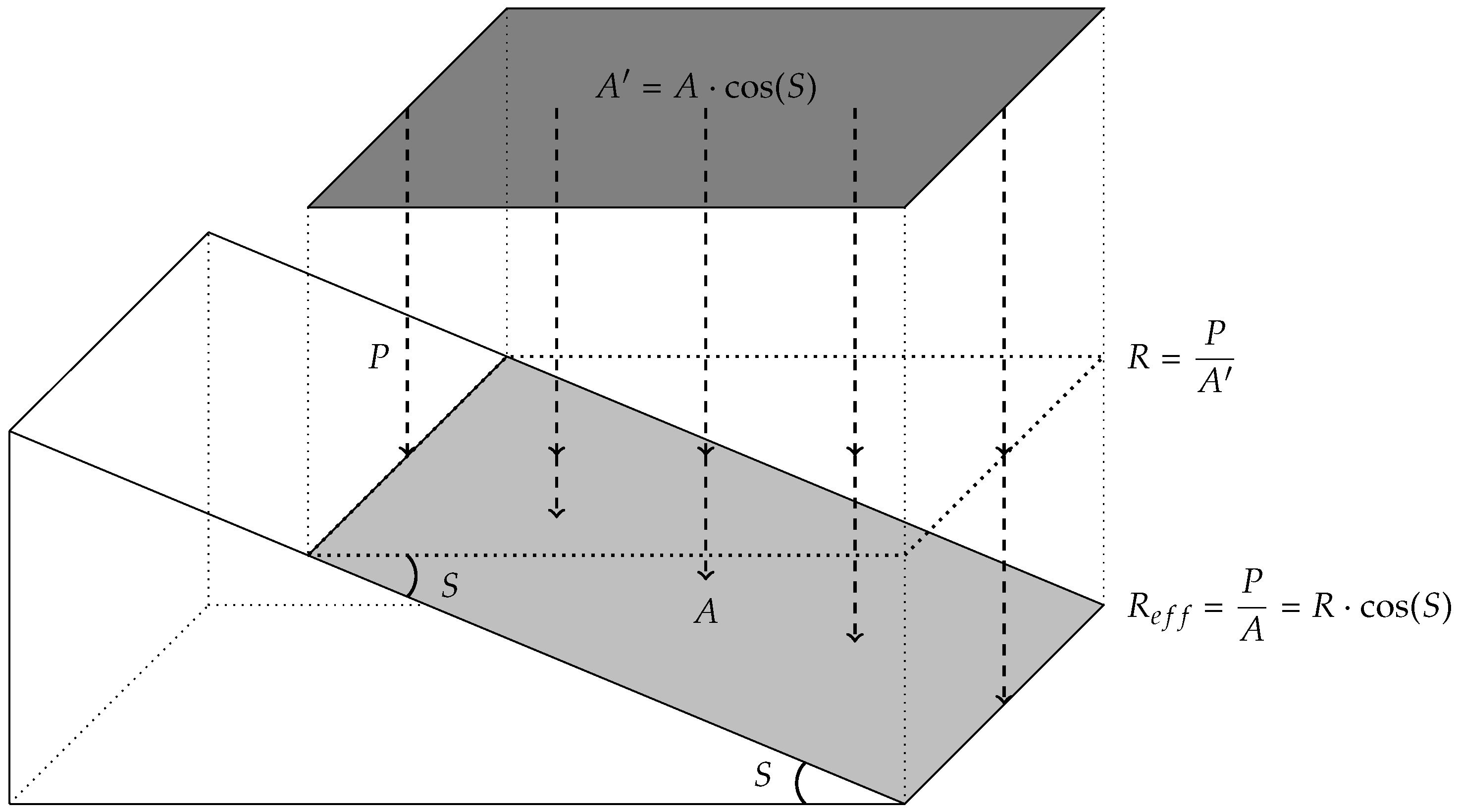
  • Revision of the effective rainfall equation, the interflow equation, and equations relevant to flow velocity.

2. Model Description

2.1. The DMMF Model

The DMMF model is a conceptual soil erosion model used to estimate surface runoff and sediment flux from a field scale on a daily basis. Spatially, the DMMF model represents an area as several interconnected elements of uniform topography, soil characteristics, land cover type, and vegetation structure. Through coupling the model with flow direction algorithms, each element receives water and sediments from upslope elements and delivers the generated surface runoff and eroded soils to downslope elements. Temporally, the model estimates the surface runoff and the sediment flux of each element on a daily basis and can extend its temporal scales through updating the model for a given period. The DMMF model estimates water and sediment flux of an element in two main phases; the hydrological phase and the sediment phase. The hydrological phase is based on the simple soil water storage approach where surface runoff occurs when daily surface water inputs exceed soil water storage capacity (i.e., saturation-excess overland flow) as outlined in Kirkby [40]. In the model, we redefined the soil water storage capacity as the surface water infiltration capacity after considering the blocking effect of impervious covers. The sediment phase is largely based on the sediment balance process from the MMMF model. Based on this framework, we redefined the flow velocity by adopting the modified Manning’s equation from Petryk and Bosmajian [41] and the transport capacity equation with the normalized flow velocity. Additionally, we changed to have all sediment input processes occur before the deposition process in order to apply deposition process for all the sediment inputs. The model is also adapted to consider the impact of impervious surface covers on runoff and sediment redistribution. The hydrological and the sediment phases of the model work with water volume ( L   m 2 = mm) and sediment weight ( k g   m 2 ) per surface area of an element, respectively. On the other hand, matter exchange between elements uses the total volume of water ( L ) and the total weight of sediment ( k g ), and considers the size difference of source areas and accepting areas. In this study, we describe the DMMF model comprehensively; although a substantial part of the model follows the MMMF model, to explain the new routines and revised processes with consistency. To distinguish the new routines and revised equations from those of the original MMMF model, we indicate unchanged MMMF equations by an asterisk next to the equation number. A detailed description of input parameters is presented in Table 1.

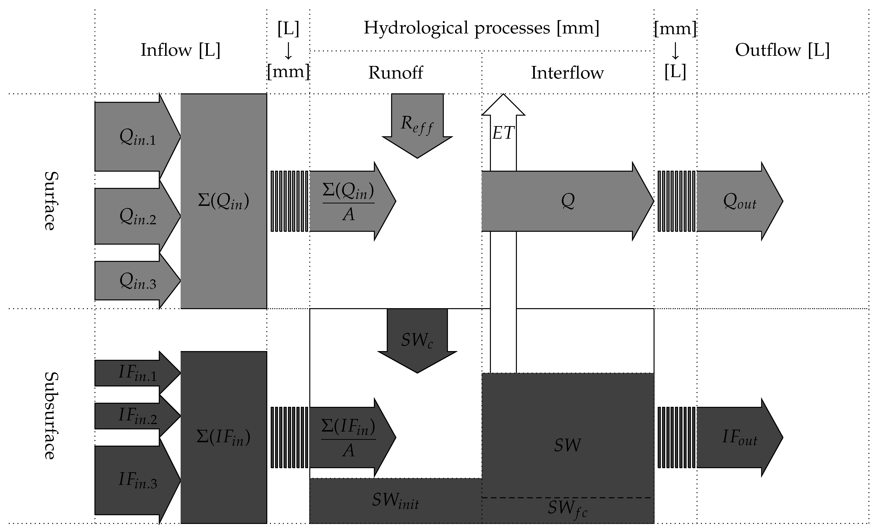
2.2. Hydrological Phase

The hydrological phase consists of two major processes: the surface runoff and the subsurface interflow processes (Figure 1). In the model, the subsurface process is simplified by conceptualizing a soil profile as one layer and adopting average hydraulic characteristics of an entire soil profile (i.e., soil water contents ( θ i n i t , θ s a t , and θ f c ), and saturated soil lateral hydraulic conductivity (K)).

2.2.1. Surface Runoff Process

The fountainhead of the hydrological process is the effective rainfall ( R e f f ; mm): the volume of rainfall reaching the unit surface area of an element. According to the corrected effective rainfall from Choi et al. [39], with the existence of natural or artificial objects that intercept rainfall before reaching the ground, the effective rainfall on a unit surface area (A; m 2 ) of an element can be described as,
R e f f = R · ( 1 P I ) · cos ( S ) ,
where P I is the proportion of the permanent interception area and S is the slope of an element. In the MMMF model, the slope adjustment factor is 1 / cos ( S ) , but it should be cos ( S ) from the trigonometric rule as described in Choi et al. [39] and in Figure 2.
The DMMF model estimates the amount of the surface runoff (Q; mm) by considering surface water infiltration capacity, surface water input, and the proportion of the impervious surface area of an element. The surface water infiltration capacity ( S W c ; mm) is the amount of surface water that can infiltrate into the subsurface layer. S W c is determined by potential pore space left for water infiltration and the proportion of the impervious surface area ( I M P ). Because impervious surface hinders infiltration of water, I M P is assumed to decrease S W c . Therefore, S W c is defined as,
S W c = ( 1 I M P ) · ( S W s a t S W i n i t Σ ( I F i n ) A ) ,
where S W s a t (mm) and S W i n i t (mm) are the amount of the saturated soil water and the initial soil water that already exist in the soil before a daily event started. Σ I F i n ( L ) is the total volume of subsurface inflow of water from upslope elements and A ( m 2 ) is the surface area of an element. Thus Σ I F i n / A (mm) represents the inflow of subsurface water per unit surface area. The first parenthesis of Equation (2) indicates the blocking effect of water infiltration by impervious covers, and the second parenthesis indicates the potential pore space left for water infiltration. The saturated and initial soil water volumes are,
S W s a t = 1000 · θ s a t · S D ,
S W i n i t = 1000 · θ i n i t · S D .
Here, θ s a t , and θ i n i t are the saturated and initial volumetric soil water contents ( vol / vol ) and S D ( m ) is the soil depth of an element. The factor of 1000 was used to convert meters to millimeters. The negative S W c indicates the return flow, which contributes to additional surface water input through upwelling when soil water inputs exceed the saturation point of soil. In the model, surface runoff occurs when surface water inputs exceed the surface water infiltration capacity of an element. The surface water inputs are the sum of the effective rainfall, and surface water contributions from upslope elements ( Σ ( Q i n ) / A ; mm). Therefore, the surface runoff of a unit surface area of an element is,
Q = R e f f + Σ ( Q i n ) A S W c .
and the total volume of surface runoff from an element ( Q o u t ; L) is,
Q o u t = Q · A .

2.2.2. Interflow Process

After the surface runoff process, the model estimates the subsurface interflow of an element ( I F o u t ), which is the volume of soil water being transferred to downslope elements. Interflow occurs when the amount of soil water budget ( S W ; mm) exceeds soil water at field capacity ( S W f c ; mm). The soil water budget is calculated considering subsurface water inputs including existing soil water, surface water infiltration, and evapotranspiration, which is equal to the total water budget of an element:
S W = ( S W i n i t + Σ ( I F i n ) A ) + ( R e f f + Σ ( Q i n ) A Q ) E T .
The formula in the first parenthesis of Equation (7) represents subsurface water inputs and the second formula parenthesis represents infiltrated surface water to the subsurface. Soil water at field capacity is defined as the amount of water-holding capacity of soil against the gravitational force based on Veihmeyer and Hendrickson [42], but the value in this model covers the entire soil profile, and not a particular layer of uniform texture. In this model, soil water at field capacity is described as,
S W f c = 1000 · θ f c · S D ,
where θ f c ( vol / vol ) is the water content at field capacity of the entire soil profile. According to the corrected interflow equation suggested by Choi et al. [39], I F o u t of an element with a width of w is described as (see details in Figure 3),
I F o u t = K · sin ( S ) · ( S W S W f c ) · w , when I F o u t < ( S W S W f c ) · A , ( S W S W f c ) · A , when I F o u t ( S W S W f c ) · A ,
for a given saturated soil lateral hydraulic conductivity (K; m   d 1 ). The volume of interflow cannot exceed the total volume of soil water budget over field capacity, which is the source of interflow. After the interflow process, a part of soil water remains in the soil. The remaining soil water content ( θ r ; vol / vol ) can then be described as,
θ r = ( S W I F o u t / A ) 1000 · S D ,
where 1000 is used to convert meters to millimeters. The DMMF model uses the measured initial soil water content just before the first day of a rainfall event and the remaining soil water content ( θ r ) replaces the initial soil water content ( θ i n i t ) of the next day when the model is applied to a period longer than a day.

2.3. Sediment Phase

The sediment phase of the model inherits the basic structure of the sediment balance process of the MMMF model. Therefore the model estimates sediment budgets of each particle size class (i.e., clay, silt, and sand) separately, considering surface conditions (e.g., vegetation structures, surface roughness, and crop field management type). The model also follows step-wise processes of the sediment detachment and deposition of the MMMF model which simplify the in-element erosion process. There are three differences in the sediment phase in this model from that of the MMMF model (Figure 4). First, the sequence of processes was changed to have all the sediment input processes occur before deposition processes. Second, we revised the flow velocity equation from four equations of the MMMF model to two equations of reference and actual flow velocities by adopting the modified Manning’s equation from Petryk and Bosmajian [41]. This modification further simplified and enhanced the conceptual clarity of the model, not only in the flow velocity equation, but also in the particle settling rates and the transport capacity calculations. Third, we changed the MMMF sediment budgeting process to that of Meyer and Wischmeier [43] as the MMMF process is motivated by longer time steps. The sediment phase comprises of three processes: sediment delivery to the surface runoff, gravitational deposition, and soil erosion processes. A schematic description of the sediment phase is given in Figure 4.

2.3.1. Sediment Delivery to Surface Runoff

In the model, surface runoff and sediments that are delivered to surface runoff are the two main factors that determine sediment loss from an element. The sources of delivered sediments are in-element detached particles by the impact of rainfall and surface runoff, as well as delivered soil particles from upslope elements. Soil detachment by rainfall occurs when raindrops fall directly onto ground surface with sufficient kinetic energy to detach soil particles from the surface. Because canopy cover changes the kinetic energy of raindrops by initializing raindrop velocity and altering raindrop size [44], rainfall has a different impact on areas under and without canopy cover. Grounds without canopy cover are affected by the raindrops falling directly onto the bare soil (direct throughfall). The kinetic energy density of direct throughfall ( U D T ; J   m 2   mm 1 ) is estimated from the universal power law equation suggested by Shin et al. [45] for a given rainfall intensity ( R I ; mm   h 1 ):
U D T = 10.3 · R I 2 / 9 .
In contrast, under the canopy cover, soil surface is affected by the water-drops falling from the leaves and stems of vegetation after rainfall (leaf drainage). The kinetic energy density of leaf drainage ( U L D ; J   m 2   mm 1 ) under a 100 canopy cover is a function of plant height ( P H ; m ) [44]:
U L D = 15.8 · P H 5.87 , when U L D 0 , 0 , when U L D < 0 .
Because U L D is kinetic energy density, its value cannot be less than zero; although the empirical equation potentially allows negative values. In an element partly covered with vegetation, the kinetic energy of the effective rainfall ( K E ; J   m 2 ) can be expressed as the product of the effective rainfall ( R e f f ) and the area weighted average of kinetic energy densities of U D T and U L D :
K E = R e f f · ( 1 C C ) · U D T + C C · U L D ,
where C C is the proportion of the canopy covered area of an element. Then, the amount of soil particles detached by raindrops (F; k g   m 2 ) is calculated as a function of detachability of soil particles by raindrop impact ( D K ; g   J 1 ), proportion of each particle size class (P), proportion of bare soil surface ( 1 E P A ), and the kinetic energy of the effective rainfall ( K E ):
F c = D K c · P c · ( 1 E P A ) · K E · 10 3 ,
F z = D K z · P z · ( 1 E P A ) · K E · 10 3 ,
F s = D K s · P s · ( 1 E P A ) · K E · 10 3 .
Here, subscripts c, z and s represent each particle size classes of clay, silt, and sand, respectively. E P A is the erosion protected area by ground cover ( G C ) and impervious area ( I M P ):
E P A = I M P + ( 1 I M P ) · G C .
The guide values for detachability of clay, silt, and sand are 0.1, 0.5, and 0.3, respectively [27] but these values should be used carefully according to the soil characteristics of study sites as shown in Poesen [46] and it is recommended that users employ field-measured values.
The second sediment source is detached soil particles by the surface runoff (H; k g   m 2 ). The amount of detached soil particles by runoff is calculated as a function of detachability of soil particles by runoff ( D R ; g   mm 1 ), the amount of runoff (Q), the slope angle (S) of the element, and the proportion of the bare surface area. Therefore, H for particle size classes are,
H c = D R c · P c · Q 1.5 · ( 1 E P A ) · ( sin ( S ) ) 0.3 · 10 3 ,
H z = D R z · P z · Q 1.5 · ( 1 E P A ) · ( sin ( S ) ) 0.3 · 10 3 ,
H s = D R s · P s · Q 1.5 · ( 1 E P A ) · ( sin ( S ) ) 0.3 · 10 3 .
The guide values for detachability of clay, silt, and sand are 1.0, 1.6, and 1.5, respectively [27]. The values should be used carefully and can be replaced with observed site specific data.
The third sediment source is sediment inputs from upslope elements ( Σ ( S L i n ) ) averaged by the surface area of an element. Therefore, the overall delivered sediments to the surface runoff ( S S ; k g   m 2 ) are represented as below,
S S c = F c + H c + Σ ( S L i n . c ) A ,
S S z = F z + H z + Σ ( S L i n . z ) A ,
S S s = F s + H s + Σ ( S L i n . s ) A .
Detached sediments can be transported by surface runoff through suspension, saltation, and creeping processes. In the model, all sediments delivered to surface runoff are assumed as being in suspension.

2.3.2. Gravitational Deposition of Suspended Sediments

After sediments are delivered to the surface runoff, a part of the suspended sediments ( S S ) in the runoff settle to the bottom by gravitational force. Tollner et al. [47] estimated the settling rate of suspended sediments using the probabilistic concept of the particle fall number ( N f ), which is the ratio of falling time of soil particles to traveling time along the flow direction of an element. To calculate the particle fall number, the runoff flow velocity (v; m   s 1 ) and settling velocity of each particle size class ( v s ; m   s 1 ) are required. Flow velocity depends on the flow depth (d), the slope of an element (S) and the modified Manning’s roughness coefficient ( n ) from Petryk and Bosmajian [41]. The modified Manning’s roughness coefficient is the hydraulic roughness considering the effect of the drag force by vegetation on the hydraulic roughness in addition to the Manning’s roughness coefficient. The value is determined by the Manning’s roughness coefficient (n), the flow depth (d), the diameter of plant stems (D) and the number of stems per unit area ( N V ) with the standard gravity of the Earth ( g 9.8 m   s 2 ):
v = 1 n · d 2 / 3 · tan ( S ) ,
n = n 2 + D · N V · d 4 / 3 2 · g 1 / 2 .
Recommended values for d are 0.005 for unchanneled flow, 0.01 for shallow rills, and 0.25 for deeper rills, but field measured flow depth can be used. For cultivated land with tillage, the Manning’s roughness coefficient can be derived empirically from the soil surface roughness ( R F R ; cm m 1 ) as below [27],
ln ( n ) = 2.1132 + 0.0349 · R F R .
Guide values of surface roughness ( R F R ) for different tillage implements are described in Morgan [3] and Morgan and Duzant [27].
The settling velocity ( v s ) is estimated from the Stokes’ equation for a creeping flow when the Reynolds number is low:
v s = δ 2 · ( ρ s ρ ) · g 18 · η .
Here, δ and ρ s are the diameter and density of a particle, and ρ and η are the density and the viscosity of a fluid. The density of each particle size class ( ρ s ) is set as 2650 k g   m 3 , which is the average density of quartz. The density of overland flow ( ρ ) is set as the density of water (1000 k g   m 3 ), and the viscosity of overland flow ( η ) is set as 0.0015 k g   m 1   s 1 following Morgan and Duzant [27]. Assuming that particle diameters are 0.2 × 10⁻⁵ m for clay, 0.6 × 10⁻⁴ m for silt, and 0.2 × 10⁻³ m for sand, then the settling velocities are 0.2 × 10⁻⁵ m   s 1 for clay ( v s . c ), 0.2 × 10⁻² m   s 1 for silt ( v s . z ), and 0.2 × 10⁻¹ m   s 1 for sand ( v s . s ) [27]. The particle fall number ( N f ) of each particle size class is a function of the actual runoff velocity (v), the settling velocities of each particle size class ( v s ), the depth of runoff (d) in meters, and the length of the element (l):
N f . c = l v · v s . c d ,
N f . z = l v · v s . z d ,
N f . s = l v · v s . s d .
Using the particle fall number of each particle size class, the rate of deposition of the sediments suspended in runoff ( D E P ) is estimated from the equation of Tollner et al. [47], as below,
D E P c = min ( 0.441 · N f . c , 1 ) ,
D E P z = min ( 0.441 · N f . z , 1 ) ,
D E P s = min ( 0.441 · N f . s , 1 ) .
Because the deposited particles cannot exceed the sediments suspended in the runoff, the maximum value for the deposition rate of each particle is set to one. After a part of the suspended sediments is deposited by gravitational force, the remaining suspended sediments become available for transport (i.e., the available sediments for transport (G) ( k g   m 2 )) by the surface runoff:
G c = S S c · ( 1 D E P c ) ,
G z = S S z · ( 1 D E P z ) ,
G s = S S s · ( 1 D E P s ) .

2.3.3. Estimation of Sediment Loss from an Element

The transport capacity of the runoff ( T C ; k g   m 2 ) of an element depends on the volume of surface runoff per unit surface area of an element (Q), the slope steepness (S) and the effect of surface conditions [27]. The effect of surface conditions is expressed as the ratio between actual runoff velocity (v) and the reference velocity of the element ( v r ; m   s 1 ). The reference velocity ( v r ) is the runoff velocity of an element under a standard surface condition (i.e., unchanneled overland flow over smooth bare soil) and is described by the Manning’s equation,
v r = 1 n r · d r 2 / 3 · tan ( S ) ,
where values of n r = 0.015 and d r = 0.005 are used for a standard surface condition. Following the corrected MMMF C-factor suggested by Choi et al. [39], the total transport capacity of the runoff is calculated as,
T C = v v r · Q 2 · sin ( S ) · 10 3 .
The transport capacity of the runoff is partitioned into clay, silt, and sand by multiplying the mass proportion of each particle size class with T C :
T C c = P c · T C ,
T C z = P z · T C ,
T C s = P s · T C .
The sediment loss from the element ( S L ) is determined by comparing the transport capacity of the runoff ( T C ) with the amount of available sediment for transport (G) [27,43]. Because this model calculates the output on a daily basis, it is better to follow the sedimentation process from Meyer and Wischmeier [43], which is appropriate for shorter time periods. When T C is greater than G, the surface runoff washes away all the sediments available for transport from an element, and in the other case, an amount of sediment ( S L ) equivalent to T C is lost from an element:
S L c = min ( T C c , G c ) ,
S L z = min ( T C z , G z ) ,
S L s = min ( T C s , G s ) .
The overall amount of sediment eroded from an element ( S L ) is the sum of clay, silt, and sand discharged from an element:
S L = S L c + S L z + S L s .

2.4. Estimation of Total Runoff and Soil Erosion for Rainfall Period

The model can estimate the total amount of surface runoff and sediment loss from an element during a rainfall period by utilizing daily input data. For long-term estimation during a rainfall period, the model requires daily values of time-variant meteorological data (R, R I , and E T ), and vegetation structure data ( G C , C C , P H , D, and N V ). On the contrary, the model requires site specific data of an element for static parameters such as topography (S, l, and w), soil characteristics ( S D , θ s a t , θ f c , D K , D R , and K), and surface conditions ( P I , I M P , and n). It is difficult to obtain daily data for the initial soil water content ( θ i n i t ), although it is highly time-variant, similar to meteorological data. To cope with the problem, the model iteratively replaces the initial soil water content ( θ i n i t ) with the remaining soil water content ( θ r after the interflow process. Through daily updates, the model estimates the surface runoff and the sediment loss from an element during a period by accumulating daily results of Q and S L for the period.

3. Testing the DMMF Model

3.1. Sensitivity Analysis of the Model

A sensitivity analysis of the DMMF model was conducted to investigate the relative importance of input parameters on the amount of surface runoff and sediment loss from an element. We analyzed the sensitivity of the model to each parameter with the Sobol’ method. The Sobol’ method is a variance-based sensitivity analysis through variance decomposition and has the advantage to estimate the total effect of a parameter including its effects in combination with other parameters [48,49,50,51]. Therefore, unlike the local and the one factor at a time (OAT) sensitivity analysis, the Sobol’ method can be applied to non-linear and non-additive models with many parameters [52,53]. Because of its advantages, the Sobol’ method has become popular in environmental and hydrological modeling that employ models such as SWAT and TOPMODEL [51,53]. The total effect of a parameter by the Sobol’ total index (SI) is the amount of total variance caused by a parameter normalized by the amount of variance induced from all parameters (unconditional variance of the model). Parameters with large SI have relatively high impacts and those with small SI have low impacts on the model output. To estimate SIs for the input parameters of the DMMF model, we set the range of the parameters based on the values recommended by Morgan and Duzant [27]. For meteorological parameters, we took extreme values to consider various weather events from a variety of regions. We set the range of the element size ( r e s ) considering various DEM resolutions, and set the complete range of the slope (S), from a flat surface to a vertical cliff. The detailed range of parameters is listed in Table 1. Sobol’ total indices for input parameters are estimated through the “sobolmartinez” function of the “sensitivity” package [54] using R version 3.2.3 [55]. We used the default bootstrapping option of the function employing a sample size of 10 5 .
According to Sobol’ total indices (Figure 5), runoff of an element is highly sensitive to the factors determining surface water infiltration capacity (i.e., θ i n i t , θ s a t , S D , and I M P ) and water input from the effective rainfall (i.e., R, S, and P I ). The amount of sediment loss from an element is also highly sensitive to the factors that show high sensitivity to surface runoff, because the amount of surface runoff is the main driver of soil redistribution. Furthermore, sediment loss of an element shows sensitivities to surface conditions ( I M P , and G C ) and vegetation structures (D, N V , and C C ). For a single element sensitivity analysis, the soil water content at field capacity ( θ f c ) and the lateral hydraulic conductivity (K) show no effects on the model because they are involved in subsurface water exchange among elements that are not considered in the sensitivity analysis for one element. These sensitivity analysis results are agree well with the model assumptions as well as conform to parameter sensitivity analysis of the MMMF model described by Morgan and Duzant [27].

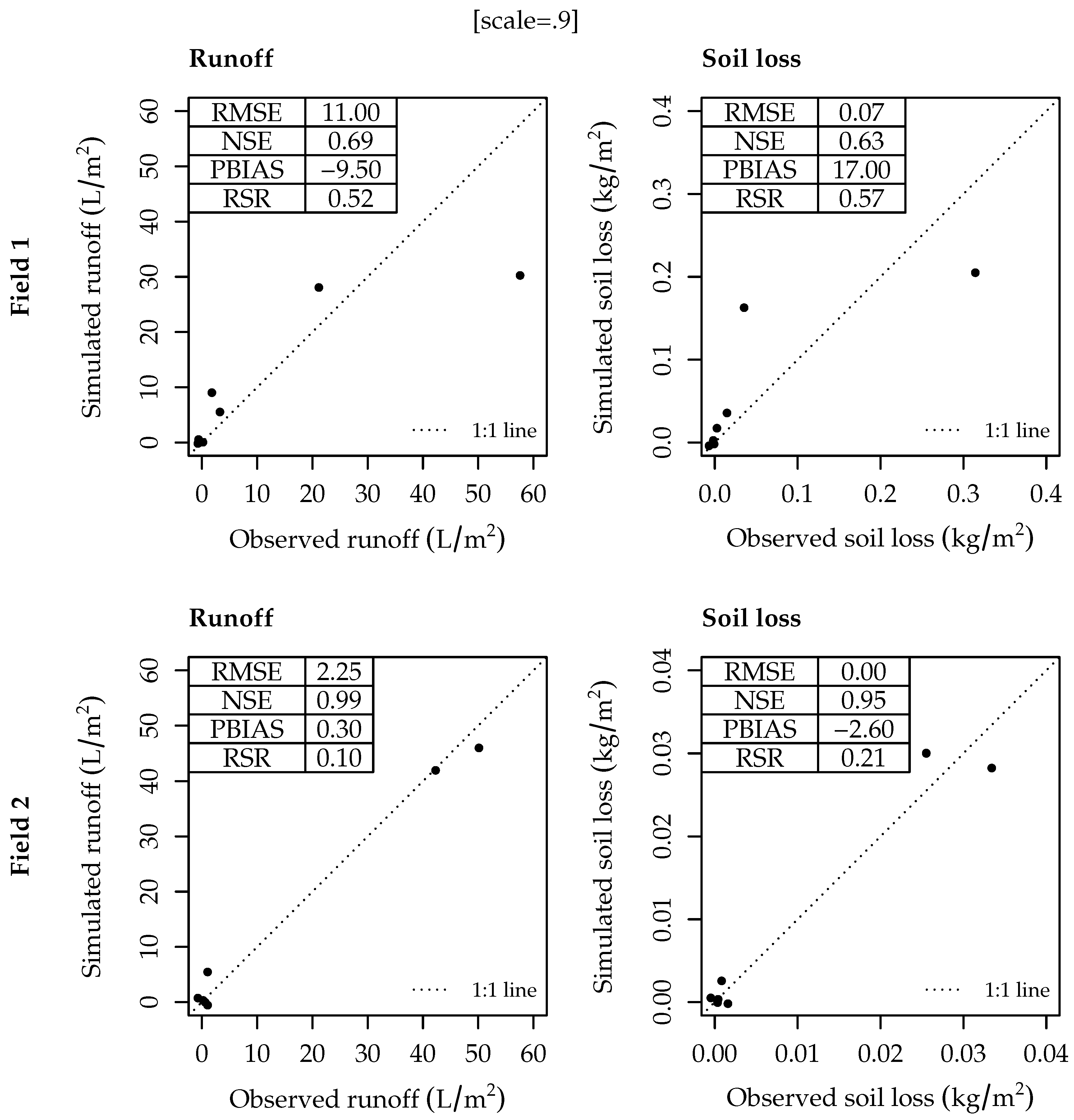
3.2. Testing the DMMF Model in the Field

We applied the DMMF model to two potato fields (field 1 and field 2) in the Haean-Myeon catchment, South Korea, previously described by Arnhold et al. [37] to test the validity of the model. The fields are located on erosion-prone hillslopes with complex surface configurations of plastic-covered ridges with potatoes and bare soil furrows. Mean annual precipitation in the study area in 2009 and 2010 was about 1514 mm, with 50% to 60% of the annual rainfall concentrated during the summer monsoon season from June to August [37]. Soils of the fields range from sandy to silty loams, with higher proportions of clay and silt in field 2. Field 1 is located on a concave hillslope with a topographical depression along the center line of the field, and the field 2 is on a concave slope without any topographical depressions. Both fields have an average slope angle of about 9 and a slope length of about 25 m . On each field, runoff and sediment loss were measured by three 5 m wide runoff samplers for seven rainfall periods with a variety of rainfall characteristics and time intervals in the monsoon season from 5 July to 10 August 2010 [37]. These conditions in both fields are suitable for testing the model at a variety of temporal rainfall periods including the new concept of impervious areas. We used available measured and estimated input parameters to test the model. Digital elevation models (for S, w and l), R, R I , S D , n, P c , P z , P s , θ i n i t , C C , and P H were obtained from Arnhold et al. [37]. For E T , we utilized the MODIS/Terra Evapotranspiration [63], because it provides an 8-day sum of ET data based on the modified Penman-Monteith equation [64]. For unmeasured input parameters ( θ s a t , θ f c , K, P I , G C , N V , D, D K c , D K z , D K s , D R c , D R z , D R s , and d), site-specific sensitivity analyses were performed to determine the required parameters to be adjusted, which is recommended under the situation of limited data availability. We selected parameters for calibration when one of their Sobol’ total index values from field 1 or field 2 was larger than 0.05 (i.e., contribute 5% of the total variance of the model output). For parameters related to soil detachability (i.e., D K c , D K z , D K s , D R c , D R z , and D R s ), we used a wide range of parameters from zero to maximum values as given in Table 1. We set the range of K according to ranges of the optimized vertical hydraulic conductivities from Ruidisch et al. [38], who conducted hydrological studies on the same fields. The upper boundary was defined by multiplying K by 18 to consider the average ratio of lateral to vertical hydraulic conductivities of the hillslope [65]. The range of d was set from 0.005 (unchanneled flow) to 0.01 (shallow rill) from Morgan and Duzant [27], considering surface conditions of both fields. Ranges of θ s a t were estimated from Saxton et al. [61] using soil texture of each field. Ranges of θ f c were derived from ranges of initial soil water content before rainfall, because excess soil water usually drained away two or three days after the soil was fully saturated by rainfall. Initial soil water contents from Arnhold et al. [37] were measured between one and three days after previous rainfall events ended. We adjusted the other parameters using a range of ±20 of guide values given in Morgan and Duzant [27]. The detailed range of parameters for sensitivity analysis is listed in Table 2.
According to the result, K, θ s a t , and θ f c showed relatively high impacts on the amount of surface runoff and sediment loss from an element. D R c , D R z , D R s and d show relatively high impacts (over 0.1) on sediment loss result (see Figure 6). These seven parameters have high in-situ variations as well [27,65,66]. We calibrated the model by adapting K, θ s a t , θ f c , D R c , D R z , D R s and d with the same range of parameters used in the sensitivity analysis. For parameters with relatively low impacts on the model results, we used reference values for potato fields from Morgan and Duzant [27].
We used the differential evolution (DE) optimization method [67] for model calibration through the “DEoptim” package [68] using R version 3.2.3 [55]. The DE algorithm is a heuristic optimization method with an evolution strategy to find the global minimum of a real-valued model of real-valued parameters. It is suitable for non-differentiable, nonlinear and multimodal models. Therefore, the DE algorithm and its variants have been successfully applied to a variety of fields [67,68,69] and have been used for hydrological model calibration [70,71]. To find the best parameter set for the model output, we used the root mean square error (RMSE) between model outputs and the field measured data as the objective function for the DE algorithm. Because the surface runoff is one of the main drivers of sediment processes, we optimized K, θ s a t , and θ f c for the surface runoff (Q) and then, with these optimized parameters, we optimized D R , and d for sediment loss ( S L ). Values of optimized parameters from the DE algorithm are listed in Table 3.
The optimized K for each field is in the range of optimized (for field 1) and estimated (for field 2) vertical hydraulic conductivity from Ruidisch et al. [38]. It means that the lateral hydraulic conductivity of the entire soil profile is affected not only by the top soil layer but also by other deeper layers with low hydraulic conductivities. The optimized θ s a t for each field has a relatively higher value than the corresponding optimized values from Ruidisch et al. [38]. The higher values are possible because the model considers the entire soil profile, including deeper soil layers with higher saturated soil water contents. The optimized θ f c values for both fields are consistent with the values for silt loam (0.35) for field 1 and silt clay loam (0.42) for field 2 from Morgan and Duzant [27]. The optimized D R values are lower than those in the ranges of D R for sensitivity analysis from Morgan and Duzant [27]. However, the optimized values are possible because the values were induced from laboratory data from Quansah [72] and possess a significant amount of uncertainty according to Morgan and Duzant [27]. Finally, the optimized d indicates that field 1 has shallow rills and field 2 has a comparatively smooth surface, which are consistent with actual field surface conditions. With the optimized parameters, we tested the model with three other statistical criteria for evaluating the model performance: the Nash-Sutcliffe efficiency (NSE), the percent bias (PBIAS), and the ratio of RMSE to the standard deviation of the observation (RSR). A model is considered to be acceptable when it has an NSE value larger than 0.5, a PBIAS value in the range ±25, and a RSR value less than or equal to 0.7 [73]. The testing results of the model are acceptable for both runoff and sediment loss (Figure 7).
The test results from field 2 show better performance than those from field 1. The putative causes of the differing model performance for two fields are data gaps due to damages of a runoff collector in field 1. This collector covered a large proportion of the field area and, thus, might have strongly affected outputs of the entire field [37]. Although data gaps were also present in field 2, contributing areas of each runoff collector were rather similar, which decreased the influence of an individual collector on the average output of the entire field (see Figure 2 and Table 2 in Arnhold et al. [37]). Further, model performance for runoff is better than that for sediment loss for both fields. The poorer performance for sediment loss than for runoff is assumed to be caused by error propagation of runoff as the main driver of sediment loss. Although more evenly distributed observed data are desirable for better model performance testing, observation data were clustered into low and high extremes due to the highly irregular rainfall pattern of the Monsoon climate and the limited period of observation.

4. Summary and Conclusions

In this study, we present a new soil erosion model, the Daily based Morgan–Morgan–Finney (DMMF) model, which is suitable for estimating surface runoff and soil erosion of a complex surface terrain within an intensive seasonal rainfall region. The DMMF model is based on the simple conceptual soil erosion model, the Modified Morgan–Morgan–Finney model, with several modifications. First, the temporal scale of the model changed from an annual to a continuous daily scale. Second, we added a new surface cover type of impervious area that highly affects runoff generation and soil redistribution patterns. Third, we revised the main equations and rearranged the sequence of the subprocesses for a better physical representation of the model. In the hydrological phase, we revised the effective rainfall and the interflow equations. In the sediment phase, we modified the flow velocity equations, the transport capacity equations, and the sediment input sequence.
Owing to these modifications, the DMMF model offers expanded temporal and spatial applicability while retaining the advantages of the MMMF model. Temporally, the model can estimate short- and long-term soil erosion flexible in regions with concentrated seasonal rainfall for which the annual-based MMMF model is not suitable. Spatially, the model can estimate runoff and soil erosion for complex surface configurations with plastic mulching, pavements and so on by introducing the proportion of the impervious area. Furthermore, the model represents the effect of vegetation on soil erosion by utilizing easy-to-measure vegetation structure information, in contrast to other soil erosion models that require either detailed vegetation information or empirical relationships between vegetation and erosion. This feature enables the model to estimate spatiotemporal patterns of runoff and soil loss from non-conventional crop fields (e.g., ginseng fields in South Korea) for which only little is known about the role of the vegetation and practices such as impervious covers on soil conservation potentials. According to the sensitivity analysis and field application results, the DMMF model showed reasonable responses to parameters, which agrees with the model assumptions. The model also showed acceptable performances for both runoff and sediment loss predictions when it was tested on two potato fields with different topographic and soil characteristics in seven different rainfall periods of the monsoon season. Those results demonstrate that the new model is capable of simulating surface runoff and soil redistribution patterns at various temporal scales of monsoonal rainfall in crop fields with impervious cover.
As more national- and continental-wide topographic, soil and land use data (e.g., European Soil Data Centre [74]) are becoming available, increasing attempts have been made to apply soil erosion models at larger scales [75]. Because the DMMF model is designed for field and catchment scales, and has not yet been tested at larger scales, it is challenging at this time to directly estimate runoff and soil erosion at national and continental scales. However, the model may contribute to large scale modeling by providing appropriate parameters on non-conventional cultivation fields where insufficient information is available, to be used in large scale model approaches such as USLE and RUSLE.
We conclude that DMMF can be useful to establish soil and water conservation measures in intensively used agricultural lands with complex surface configurations composed of multiple crop types, artificial structures, and plastic mulching by estimating spatiotemporal runoff and sediment redistributions and by identifying erosion and deposition hotspots under varying conditions. Since model performance to date was tested for a single land use type and with a limited amount of observation data with data gaps, further studies are required to validate the model’s utility at extended temporal and spatial scales under various rainfall patterns and land use types as well as to provide appropriate parameterizations of non-conventional crop fields for large scale modeling.

Acknowledgments

This study is part of the International Research Training Group “Complex Terrain and Ecological Heterogeneity” (TERRECO) (GRK 1565/1) funded by the German Research Foundation (DFG). This publication was funded by the German Research Foundation (DFG) and the University of Bayreuth in the funding programme Open Access Publishing. We would like to thank Editage (www.editage.co.kr) for English language editing.

Author Contributions

Björn Reineking and Bernd Huwe designed and supervised the model algorithm and edited the manuscript. Sebastian Arnhold provided the field data for model testing, supervised the field application analysis of the model, and edited the manuscript. Kwanghun Choi designed and developed the model, analyzed the field application of the model, and wrote the paper.

Conflicts of Interest

The authors declare no conflict of interest. The founding sponsors had no role in the design of the study; in the collection, analyses, or interpretation of data; in the writing of the manuscript, and in the decision to publish the results.

References

  1. Pimentel, D.; Kounang, N. Ecology of soil erosion in ecosystems. Ecosystems 1998, 1, 416–426. [Google Scholar] [CrossRef]
  2. Sidle, R.C.; Ziegler, A.D.; Negishi, J.N.; Nik, A.R.; Siew, R.; Turkelboom, F. Erosion processes in steep terrain—Truths, myths, and uncertainties related to forest management in Southeast Asia. For. Ecol. Manage. 2006, 224, 199–225. [Google Scholar] [CrossRef]
  3. Morgan, R.P.C. Soil Erosion and Conservation, 3rd ed.; Blackwell Publishing: Malden, MA, USA, 2005. [Google Scholar]
  4. Onori, F.; De Bonis, P.; Grauso, S. Soil erosion prediction at the basin scale using the revised universal soil loss equation (RUSLE) in a catchment of Sicily (southern Italy). Environ. Geol. 2006, 50, 1129–1140. [Google Scholar] [CrossRef]
  5. Napoli, M.; Cecchi, S.; Orlandini, S.; Mugnai, G.; Zanchi, C.A. Simulation of field-measured soil loss in Mediterranean hilly areas (Chianti, Italy) with RUSLE. Catena 2016, 145, 246–256. [Google Scholar] [CrossRef]
  6. Zema, D.A.; Denisi, P.; Taguas Ruiz, E.V.; Gómez, J.A.; Bombino, G.; Fortugno, D. Evaluation of Surface Runoff Prediction by AnnAGNPS Model in a Large Mediterranean Watershed Covered by Olive Groves. Land Degrad. Dev. 2016, 27, 811–822. [Google Scholar] [CrossRef]
  7. Huon, S.; Evrard, O.; Gourdin, E.; Lefévre, I.; Bariac, T.; Reyss, J.L.; des Tureaux, T.H.; Sengtaheuanghoung, O.; Ayrault, S.; Ribolzi, O. Suspended sediment source and propagation during monsoon events across nested sub-catchments with contrasted land uses in Laos. J. Hydrol. Reg. Stud. 2017, 9, 69–84. [Google Scholar] [CrossRef]
  8. Boardman, J. Soil erosion science: Reflections on the limitations of current approaches. Catena 2006, 68, 73–86. [Google Scholar] [CrossRef]
  9. Hu, L.J.; Flanagan, D.C. Towards new-generation soil erosion modeling: Building a unified omnivorous model. J. Soil Water Conserv. 2013, 68, 100A–103A. [Google Scholar] [CrossRef]
  10. Wischmeier, W.H.; Smith, D.D. Predicting rainfall erosion losses—A guide to conservation planning. In Agriculture Handbook; Number 537, United States Department of Agriculture (USDA): Washington, DC, USA, 1978; pp. 1–58. [Google Scholar]
  11. Renard, K.G.; Foster, G.R.; Weesies, G.A.; Porter, J.P. RUSLE: Revised universal soil loss equation. J. Soil Water Conserv. 1991, 46, 30–33. [Google Scholar]
  12. Williams, J.R. Sediment-yield prediction with Universal Equation using runoff energy factor. In Present and prospective technology for predicting sediment yield and sources: Proceedings of the Sediment-Yield Workshop; United States Department of Agriculture (USDA): New Orleans, LA, USA, 1975; Volume ARS-S-40, pp. 244–252. [Google Scholar]
  13. Morgan, R.P.C.; Morgan, D.D.V.; Finney, H.J. A predictive model for the assessment of soil erosion risk. J. Agric. Eng. Res. 1984, 30, 245–253. [Google Scholar] [CrossRef]
  14. Morgan, R.P.C. A simple approach to soil loss prediction: A revised Morgan–Morgan–Finney model. Catena 2001, 44, 305–322. [Google Scholar] [CrossRef]
  15. Lal, R. Soil degradation by erosion. Land Degrad. Dev. 2001, 12, 519–539. [Google Scholar] [CrossRef]
  16. Merritt, W.; Letcher, R.; Jakeman, A. A review of erosion and sediment transport models. Environ. Modell. Softw. 2003, 18, 761–799. [Google Scholar] [CrossRef]
  17. Lilhare, R.; Garg, V.; Nikam, B. Application of GIS-Coupled Modified MMF Model to Estimate Sediment Yield on a Watershed Scale. J. Hydrol. Eng. 2014, 20, C5014002. [Google Scholar] [CrossRef]
  18. Avwunudiogba, A.; Hudson, P.F. A Review of Soil Erosion Models with Special Reference to the needs of Humid Tropical Mountainous Environments. Eur. J. Sustain. Dev. 2014, 3, 299–310. [Google Scholar] [CrossRef]
  19. Morgan, R.P.C.; Quinton, J.N.; Smith, R.E.; Govers, G.; Poesen, J.W.A.; Auerswald, K.; Chisci, G.; Torri, D.; Styczen, M.E. The European Soil Erosion Model (EUROSEM): A dynamic approach for predicting sediment transport from fields and small catchments. Earth Surf. Processes Landforms 1998, 23, 527–544. [Google Scholar] [CrossRef]
  20. De Roo, A.P.J.; Wesseling, C.G.; Ritsema, C.J. LISEM: A single-event physically based hydrological and soil erosion model for drainage basins. I: Theory, Input and Output. Hydrol. Processes 1996, 10, 1107–1117. [Google Scholar] [CrossRef]
  21. von Werner, M. GIS-orientierte Methoden der digitalen Reliefanalyse zur Modellierung von Bodenerosion in kleinen Einzugsgebieten. Ph.D. Thesis, Department of Earth Sciences, Free University of Berlin, Berlin, Germany, 1995. [Google Scholar]
  22. Nearing, M.A.; Foster, G.R.; Lane, L.J.; Finkner, S.C. A process-based soil erosion model for USDA-Water Erosion Prediction Project technology. Trans. ASAE 1989, 32, 1587–1593. [Google Scholar] [CrossRef]
  23. Beasley, D.B.; Huggins, L.F.; Monke, E.J. ANSWERS: A Model for Watershed Planning. Trans. ASAE 1980, 23, 938–944. [Google Scholar] [CrossRef]
  24. Beven, K.J.; Kirkby, M.J. A physically based, variable contributing area model of basin hydrology. Hydrol. Sci. Bull. 1979, 24, 43–69. [Google Scholar] [CrossRef]
  25. Bergström, S.; Forsman, A. Development of a conceptual deterministic rainfall-runoff model. Nord. Hydrol. 1973, 4, 147–170. [Google Scholar]
  26. Devia, G.K.; Ganasri, B.; Dwarakish, G. A Review on Hydrological Models. Aquat. Procedia 2015, 4, 1001–1007. [Google Scholar] [CrossRef]
  27. Morgan, R.P.C.; Duzant, J.H. Modified MMF (Morgan–Morgan–Finney) model for evaluating effects of crops and vegetation cover on soil erosion. Earth Surf. Processes Landforms 2008, 32, 90–106. [Google Scholar] [CrossRef]
  28. De Jong, S.M.; Paracchini, M.L.; Bertolo, F.; Folving, S.; Megier, J.; De Roo, A.P.J. Regional assessment of soil erosion using the distributed model SEMMED and remotely sensed data. Catena 1999, 37, 291–308. [Google Scholar] [CrossRef]
  29. Vigiak, O.; Okoba, B.O.; Sterk, G.; Groenenberg, S. Modelling catchment-scale erosion patterns in the East African Highlands. Earth Surf. Processes Landforms 2005, 30, 183–196. [Google Scholar] [CrossRef]
  30. López-Vicente, M.; Navas, A.; Machín, J. Modelling soil detachment rates in rainfed agrosystems in the south-central Pyrenees. Agric. Water Manage. 2008, 95, 1079–1089. [Google Scholar] [CrossRef]
  31. Vieira, D.C.S.; Prats, S.A.; Nunes, J.P.; Shakesby, R.A.; Coelho, C.O.A.; Keizer, J.J. Modelling runoff and erosion, and their mitigation, in burned Portuguese forest using the revised Morgan–Morgan–Finney model. For. Ecol. Manage. 2014, 314, 150–165. [Google Scholar] [CrossRef]
  32. Baartman, J.E.; Jetten, V.G.; Ritsema, C.J.; de Vente, J. Exploring effects of rainfall intensity and duration on soil erosion at the catchment scale using openLISEM: Prado catchment, SE Spain. Hydrol. Processes 2012, 26, 1034–1049. [Google Scholar] [CrossRef]
  33. Stocker, T.F.; Qin, D.; Plattner, G.K.; Alexander, L.V.; Allen, S.K.; Bindoff, N.L.; Bréon, F.M.; Church, J.A.; Cubasch, U.; Emori, S.; et al. Climate Change 2013: The Physical Science Basis. Contribution of Working Group I to the Fifth Assessment Report of the Intergovernmental Panel on Climate Change; Cambridge University Press: Cambridge, UK; New York, NY, USA, 2013; chapter Technical Summary; pp. 33–115. [Google Scholar]
  34. Espí, E.; Salmerón, A.; Fontecha, A.; García, Y.; Real, A.I. Plastic Films for Agricultural Applications. J. Plast. Film Sheeting 2006, 22, 85–102. [Google Scholar] [CrossRef]
  35. Shuster, W.D.; Bonta, J.; Thurston, H.; Warnemuende, E.; Smith, D.R. Impacts of impervious surface on watershed hydrology: A review. Urban Water J. 2005, 2, 263–275. [Google Scholar] [CrossRef]
  36. Pappas, E.A.; Smith, D.R.; Huang, C.; Shuster, W.D.; Bonta, J.V. Impervious surface impacts to runoff and sediment discharge under laboratory rainfall simulation. Catena 2008, 72, 146–152. [Google Scholar] [CrossRef]
  37. Arnhold, S.; Ruidisch, M.; Bartsch, S.; Shope, C.; Huwe, B. Simulation of runoff patterns and soil erosion on mountainous farmland with and without plastic-covered ridge-furrow cultivation in South Korea. Trans. ASABE 2013, 56, 667–679. [Google Scholar] [CrossRef]
  38. Ruidisch, M.; Kettering, J.; Arnhold, S.; Huwe, B. Modeling water flow in a plastic mulched ridge cultivation system on hillslopes affected by South Korean summer monsoon. Agric. Water Manage. 2013, 116, 204–217. [Google Scholar] [CrossRef]
  39. Choi, K.; Huwe, B.; Reineking, B. Commentary on ‘Modified MMF (Morgan–Morgan–Finney) model for evaluating effects of crops and vegetation cover on soil erosion’ by Morgan and Duzant (2008). Available online: https://arxiv.org/abs/1612.08899 (accessed on 13 April 2017).
  40. Kirkby, M.J. Hydrological Slope Models: The Influence of Climate. In Geomorphology and Climate; Derbyshire, E., Ed.; Wiley: London, UK, 1976; pp. 247–267. [Google Scholar]
  41. Petryk, S.; Bosmajian, G. Analysis of flow through vegetation. ASCE J. Hydraul. Div. 1975, 101, 871–884. [Google Scholar]
  42. Veihmeyer, F.J.; Hendrickson, A.H. The moisture equivalent as a measure of the field capacity of soils. Soil Sci. 1931, 32, 181–194. [Google Scholar] [CrossRef]
  43. Meyer, L.D.; Wischmeier, W.H. Mathematical simulation of the process of soil erosion by water. Trans. ASAE 1969, 12, 754–758. [Google Scholar]
  44. Brandt, C.J. Simulation of the size distribution and erosivity of raindrops and throughfall drops. Earth Surf. Processes Landforms 1990, 15, 687–698. [Google Scholar] [CrossRef]
  45. Shin, S.S.; Park, S.D.; Choi, B.K. Universal Power Law for Relationship between Rainfall Kinetic Energy and Rainfall Intensity. Adv. Meteorol. 2016, 2016, 2494681. [Google Scholar] [CrossRef]
  46. Poesen, J. An improved splash transport model. Z. Geomorphol. 1985, 29, 193–211. [Google Scholar]
  47. Tollner, E.W.; Barfield, B.J.; Haan, C.T.; Kao, T.Y. Suspended Sediment Filtration Capacity of Simulated Vegetation. Trans. ASAE 1976, 19, 678–682. [Google Scholar] [CrossRef]
  48. Sobol’, I. Sensitivity Analysis for Nonlinear Mathematical Models. Math. Model. Comput. Exp. 1993, 1, 407–414. [Google Scholar]
  49. Saltelli, A. Making best use of model evaluations to compute sensitivity indices. Comput. Phys. Commun. 2002, 145, 280–297. [Google Scholar] [CrossRef]
  50. Saltelli, A.; Annoni, P.; Azzini, I.; Campolongo, F.; Ratto, M.; Tarantola, S. Variance based sensitivity analysis of model output. Design and estimator for the total sensitivity index. Comput. Phys. Commun. 2010, 181, 259–270. [Google Scholar] [CrossRef]
  51. Qi, W.; Zhang, C.; Chu, J.; Zhou, H. Sobol’ ’s sensitivity analysis for TOPMODEL hydrological model: A case study for the Biliu River Basin, China. J. Hydrol. Environ. Res. 2013, 1, 1–10. [Google Scholar]
  52. Saltelli, A.; Annoni, P. How to avoid a perfunctory sensitivity analysis. Environ. Modell. Softw. 2010, 25, 1508–1517. [Google Scholar] [CrossRef]
  53. Nossent, J.; Elsen, P.; Bauwens, W. Sobol’ sensitivity analysis of a complex environmental model. Environ. Modell. Softw. 2011, 26, 1515–1525. [Google Scholar] [CrossRef]
  54. Pujol, G.; Iooss, B.; Janon, A.; Boumhaout, K.; Da Veiga, S.; Fruth, J.; Gilquin, L.; Guillaume, J.; Le Gratiet, L.; Lemaitre, P.; et al. Sensitivity: Global Sensitivity Analysis of Model Outputs, R package version 1.12.1; Available online: https://CRAN.R-project.org/package=sensitivity (accessed on 15 May 2016).
  55. R Development Core Team. R: A Language and Environment for Statistical Computing; R Foundation for Statistical Computing: Vienna, Austria, 2015. [Google Scholar]
  56. World Meteorological Organization’s World Weather & Climate Extremes Archive. Available online: wmo.asu.edu/content/world-meteorological-organization-global-weather-climate-extremes-archive (accessed on 16 November 2016).
  57. Senay, G.; Verdin, J.; Lietzow, R.; Melesse, A. Global Daily Reference Evapotranspiration Modeling and Evaluation. J. Am. Water Resour. Assoc. 2008, 44, 969–979. [Google Scholar] [CrossRef]
  58. Jia, L.; Xi, G.; Liu, S.; Huang, C.; Yan, Y.; Liu, G. Regional estimation of daily to annual regional evapotranspiration with MODIS data in the Yellow River Delta wetland. Hydrol. Earth Syst. Sci. 2009, 13, 1775–1787. [Google Scholar] [CrossRef]
  59. Pandey, A.; Mathur, A.; Mishra, S.K.; Mal, B.C. Soil erosion modeling of a Himalayan watershed using RS and GIS. Environ. Earth Sci. 2009, 59, 399–410. [Google Scholar] [CrossRef]
  60. Canadell, J.; Jackson, R.B.; Ehleringer, J.B.; Mooney, H.A.; Sala, O.E.; Schulze, E.D. Maximum rooting depth of vegetation types at the global scale. Oecologia 1996, 108, 583–595. [Google Scholar] [CrossRef] [PubMed]
  61. Saxton, K.E.; Rawls, W.J.; Romberger, J.S.; Papendick, R.I. Estimating generalized soil-water characteristics from texture. Soil Sci. Soc. Am. J. 1986, 50, 1031–1036. [Google Scholar] [CrossRef]
  62. Irmay, S. Hydrodynamics in soils. In Physical Principles of Water Percolation and Seepage; Bear, J., Zaslavsky, D., Irmay, S., Eds.; UNESCO: Paris, France, 1968; Volume 29, p. 60. [Google Scholar]
  63. MODIS Collection 5 Land Products Global Subsetting and Visualization Tool; ORNL DAAC: Oak Ridge, TN, USA, 2009; Available online: http://dx.doi.org/10.3334/ORNLDAAC/1241 (accessed on 22 September 2015).
  64. Mu, Q.; Zhao, M.; Running, S.W. Improvements to a MODIS global terrestrial evapotranspiration algorithm. Remote Sens. Environ. 2011, 115, 1781–1800. [Google Scholar] [CrossRef]
  65. Brooks, E.S.; Boll, J.; McDaniel, P.A. A hillslope-scale experiment to measure lateral saturated hydraulic conductivity. Water Resour. Res. 2004, 40, W04208. [Google Scholar] [CrossRef]
  66. Boll, J.; Brooks, E.S.; Campbell, C.R.; Stockle, C.O.; Young, S.K.; Hammel, J.E.; McDaniel, P.A. Progress toward development of a GIS based water quality management tool for small rural watersheds: Modification and application of a distributed model. In Proceedings of the ASAE Annual International Meeting, Orlando, FL, USA, 12–16 July 1998. [Google Scholar]
  67. Storn, R.; Price, K. Differential Evolution—A Simple and Efficient Heuristic for global Optimization over Continuous Spaces. J. Global Optim. 1997, 11, 341–359. [Google Scholar] [CrossRef]
  68. Ardia, D.; Mullen, K.M.; Peterson, B.G.; Ulrich, J. DEoptim: Differential Evolution in R, R package version 2.2-3; Available online: http://CRAN.R-project.org/package=DEoptim (accessed on 11 November 2016).
  69. Mullen, K.; Ardia, D.; Gil, D.; Windover, D.; Cline, J. DEoptim: An R Package for Global Optimization by Differential Evolution. J. Stat. Softw. 2011, 40, 1–26. [Google Scholar] [CrossRef]
  70. Joseph, J.; Guillaume, J. Using a parallelized MCMC algorithm in R to identify appropriate likelihood functions for SWAT. Environ. Modell. Softw. 2013, 46, 292–298. [Google Scholar] [CrossRef]
  71. Zheng, F.; Zecchin, A.C.; Simpson, A.R. Investigating the run-time searching behavior of the differential evolution algorithm applied to water distribution system optimization. Environ. Modell. Softw. 2015, 69, 292–307. [Google Scholar] [CrossRef]
  72. Quansah, C. Laboratory Experimentation for the Statistical Derivation of Equations for Soil Erosion Modelling and Soil Conservation Design. Ph.D. Thesis, Cranfield Institute of Technology, England, UK, April 1982. [Google Scholar]
  73. Moriasi, D.N.; Arnold, J.G.; Van Liew, M.W.; Bingner, R.L.; Harmel, R.D.; Veith, T.L. Model evaluation guidelines for systematic quantification of accuracy in watershed simulations. Trans. ASABE 2007, 50, 885–900. [Google Scholar] [CrossRef]
  74. Panagos, P.; Liedekerke, M.V.; Jones, A.; Montanarella, L. European Soil Data Centre: Response to European policy support and public data requirements. Land Use Policy 2012, 29, 329–338. [Google Scholar] [CrossRef]
  75. Panagos, P.; Borrelli, P.; Poesen, J.; Ballabio, C.; Lugato, E.; Meusburger, K.; Montanarella, L.; Alewell, C. The new assessment of soil loss by water erosion in Europe. Environ. Sci. Policy 2015, 54, 438–447. [Google Scholar] [CrossRef]
Figure 1. Schematic hydrological processes within an element. The hydrological phase estimates the amount of surface runoff (Q; mm) and subsurface interflow ( I F o u t ; L ) generated from an element. Assuming that the surface area of an element is A ( m 2 ), surface water inputs of an element is the effective rainfall ( R e f f ; mm) and surface water contribution from upslope elements ( Σ ( Q i n ) / A ; mm). Surface runoff occurs when surface water inputs exceed surface water infiltration capacity, ( S W c ; mm) which depends on available soil pore space left for surface water infiltration and the proportion of the impervious surface area ( I M P ). The subsurface interflow occurs when the soil water budget ( S W ; mm) exceeds the soil water at field capacity ( S W f c ; mm). In this condition, a part of the excess soil water outflows from an element as an interflow, and the surface runoff and subsurface interflow generated in an element are discharged to downslope elements.
Water 09 00278 g001
Figure 2. Conceptual representation of the effective rainfall ( R e f f ) on a slope element without permanent interception of rainfall (modified from Figure 1 of Choi et al. [39]). Given rainfall with a total volume of P, the amount of rainfall per unit area for both A ( m 2 ) and A ( m 2 ) is P / A and P / A which is equal to R. From the trigonometric rule, A, the projected area of A on the slope, is described as A / cos ( S ) . Therefore, the rainfall per unit surface area of the element (i.e., the effective rainfall) should be R · cos ( S ) .
Water 09 00278 g002
Figure 3. Conceptual representation of interflow in an element (modified from Figure 3 of Choi et al. [39]). Let’s assume that there is an element with the width of w, the length of l and slope of S. Then, given transferable soil water for interflow ( S W S W f c ) and saturated soil lateral hydraulic conductivity (K), the volume of interflow from the element ( I F o u t ) can be represented as K · sin ( S ) · ( S W S W f c ) · w , and cannot exceed the volume of the transferable soil water of the element ( ( S W S W f c ) · A ).
Water 09 00278 g003
Figure 4. Schematic sediment phase of an element. The model estimates the amount of sediment loss from an element through three steps. In the first step, detached soil particles from an element (by raindrop (F) and runoff (H)) and sediment inputs from upslope elements ( Σ ( S L i n ) / A ) are delivered to the surface water of an element. Second, some of the suspended sediments ( S S ) delivered in the runoff settle down due to gravity at the deposition rate of the suspended sediments in the runoff ( D E P ). Third, the model estimates the amount of sediment loss from an element by comparing the transport capacity of the runoff ( T C ) and sediments available for transport (G), which are the remaining suspended sediments after gravitational deposition process. If T C is larger than G, all the remaining sediments in the water (i.e., G) are washed away from an element. Otherwise, the amount of sediments equal to T C is carried out by the surface runoff to downslope elements.
Water 09 00278 g004
Figure 5. Sobol’ total indices of model input parameters for a single element. The bars indicate the Sobol’ total indices and the error bars indicate the 95% confidence intervals of the indices from bootstrapping.
Water 09 00278 g005
Figure 6. Sobol’ total indices for runoff (Q) and sediment loss ( S L ) of the two field sites. Bars indicate the Sobol’ total indices and the error bars indicate the 95% confidence intervals of the indices from bootstrapping. We checked the sensitivity of the model to the parameters with high uncertainty due to absence of field data, such as parameters related to soil detachability (i.e., D K c , D K z , D K s , D R c , D R z , and D R s ), soil hydraulic parameters (i.e., K, θ s a t , and θ f c ), vegetation structural parameters (i.e., G C , D, N V ), the permanent interception ( P I ), and the rill depth (d). K, θ s a t and θ f c showed relatively high impacts on the runoff (Q) and the sediment loss ( S L ). The sediment loss ( S L ) also showed high sensitivity to D R c , D R z , D R s and d.
Water 09 00278 g006
Figure 7. Comparison between simulated and observed runoff (Q) and sediment loss ( S L ) for field 1 and field 2. We tested the model performance for both fields with optimized parameters (Table 3). Model performance was evaluated using the Nash-Sutcliffe efficiency coefficient (NSE), percent bias (PBIAS), and RMSE-observation standard deviation ratio (RSR) with the observed data from Arnhold et al. [37]. To make all overlapping points with values close to zero visible, we slightly jitterred the points.
Water 09 00278 g007
Table 1. Input parameters and their range for sensitivity analysis.
ParameterDescriptionUnitRange
RDaily rainfall[mm]1–1825 (a)
R I Mean rainfall intensity of a day[mm h 1 ]15.0–305.0 (a)
E T Daily evapotranspiration[mm]0.0–15.0 (b)
SSlope angle[ rad ]0.0–1.5 (c)
r e s Grid size of a raster map for the width (w) and the length (l)of an element that are equal to r e s and r e s / cos ( S ) [ m ]0.25–100 (d)
P c Proportion of clay of the surface soil[proportion]0–1
P z Proportion of silt of the surface soil[proportion]0–1
P s Proportion of sand of the surface soil[proportion]0–1
S D Soil depth[ m ]0.3–68.0 (e)
θ i n i t Initial soil water content of entire soil profile[ vol / vol ]0.00– θ s a t (f)
θ s a t Saturated water content of entire soil profile[ vol / vol ]0.31–0.56 (f)
θ f c Soil water content at field capacity of entire soil profiles[ vol / vol ]0.10– θ s a t (f)
KSaturated soil lateral hydraulic conductivity[ m   d 1 ]1–230 (g)
D K c Detachability of clay particles by rainfall[ g   J 1 ]0.10–1.50 (h)
D K z Detachability of silt particles by rainfall[ g   J 1 ]0.50–5.15 (h)
D K s Detachability of sand particles by rainfall[ g   J 1 ]0.15–4.15 (h)
D R c Detachability of clay particles by surface runoff[ g   mm 1 ]0.020–2.0 (h)
D R z Detachability of silt particles by surface runoff[ g   mm 1 ]0.016–1.6 (h)
D R s Detachability of sand particles by surface runoff[ g   mm 1 ]0.015–1.5 (h)
P I Area proportion of the permanent interception of rainfall[proportion]0–1
I M P Area proportion of the impervious ground cover[proportion]0–1
G C Area proportion of the ground cover of the soil surfaceprotected by vegetation or crop cover on the ground[proportion]0–1
C C Area proportion of the canopy cover of the soil surfaceprotected by vegetation or crop canopy[proportion]0–1
P H Average height of vegetation or crop cover of an elementwhere leaf drainage starts to fall[ m ]0–30 (h)
DAverage diameter of individual plant elements at the surface[ m ]0.00001–3.0 (h)
N V Number of individual plant elements per unit area[ number / m 2 ]0.00001–2000 (h)
dTypical flow depth of surface runoff in an element[ m ]0.005–3 (h)
nManning’s roughness coefficient of the soil surface[ s   m 1 / 3 ]0.01–0.05 (i)
Notes: (a) is based on WMO [56]; (b) is based on Senay et al. [57], Jia et al. [58]; (c) represents the range of slope from a flat surface to a vertical cliff; (d) is based on Lilhare et al. [17], Arnhold et al. [37], Pandey et al. [59]; (e) is based on the range of rooting depth from Canadell et al. [60]; (f) is based on Saxton et al. [61]; (g) is based on the hydraulic conductivity of semi-pervious soils from Irmay [62]; (h) is based on Morgan and Duzant [27]; (i) is based on Manning’s n of bare soil in Table 3.6 from Morgan [3].
Table 2. Range of unmeasured parameters for sensitivity analysis.
Field θ sat θ fc K PI GC NV D DK c DK z DK s DR c DR z DR s d
Field 1Sup.0.4540.35117.90.1440.485.40.121.505.154.152.01.61.50.010
Inf.0.3510.3450.290.0960.323.60.080000000.005
Field 2Sup.0.4940.4355.220.1440.485.40.121.505.154.152.01.61.50.010
Inf.0.4350.4070.150.0960.323.60.080000000.005
* Sup. indicates upper bound of a range (Supremum) and Inf. indicates lower bound of a range (Infimum).
Table 3. Optimized parameters from the DE algorithm.
K θ sat θ fc DR c DR z DR s d
Field 10.5000.3620.3450.0150.0120.0110.010
Field 20.2840.4530.4350.0070.0050.0050.005

