Melting Characteristics of Snow Cover on Tidewater Glaciers in Hornsund Fjord, Svalbard


Abstract
:1. Introduction
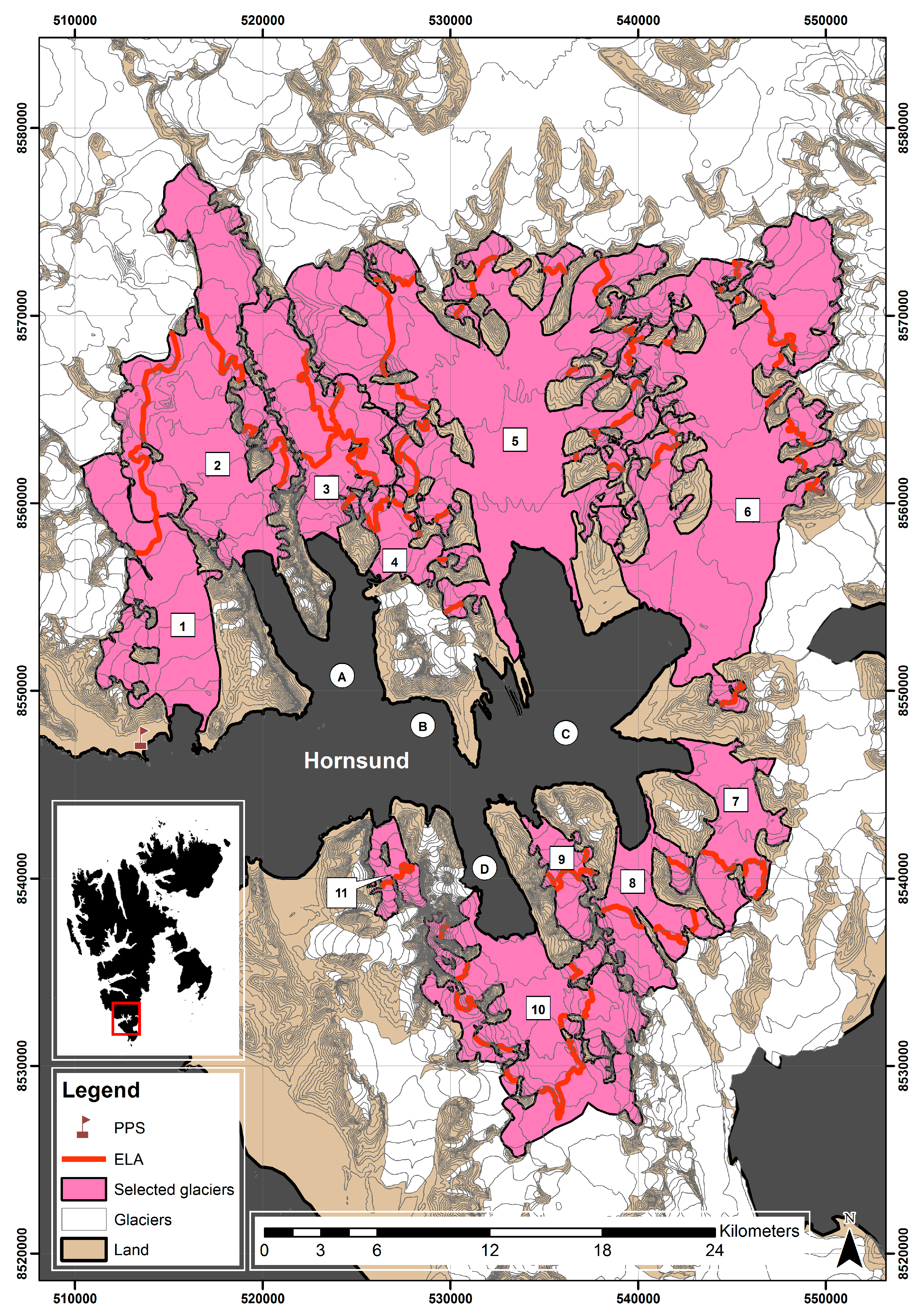
2. Study Area
3. Materials and Methods
4. Results
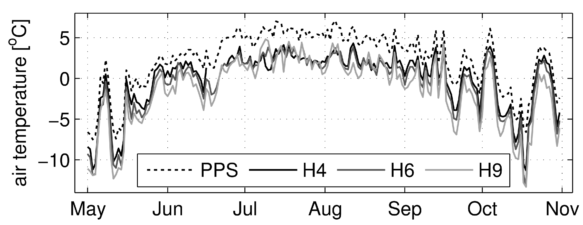
4.1. Microclimate and Topographic Determinants of the Structure of the Snow Cover on Hornsund Glaciers and Its Melting Characteristics
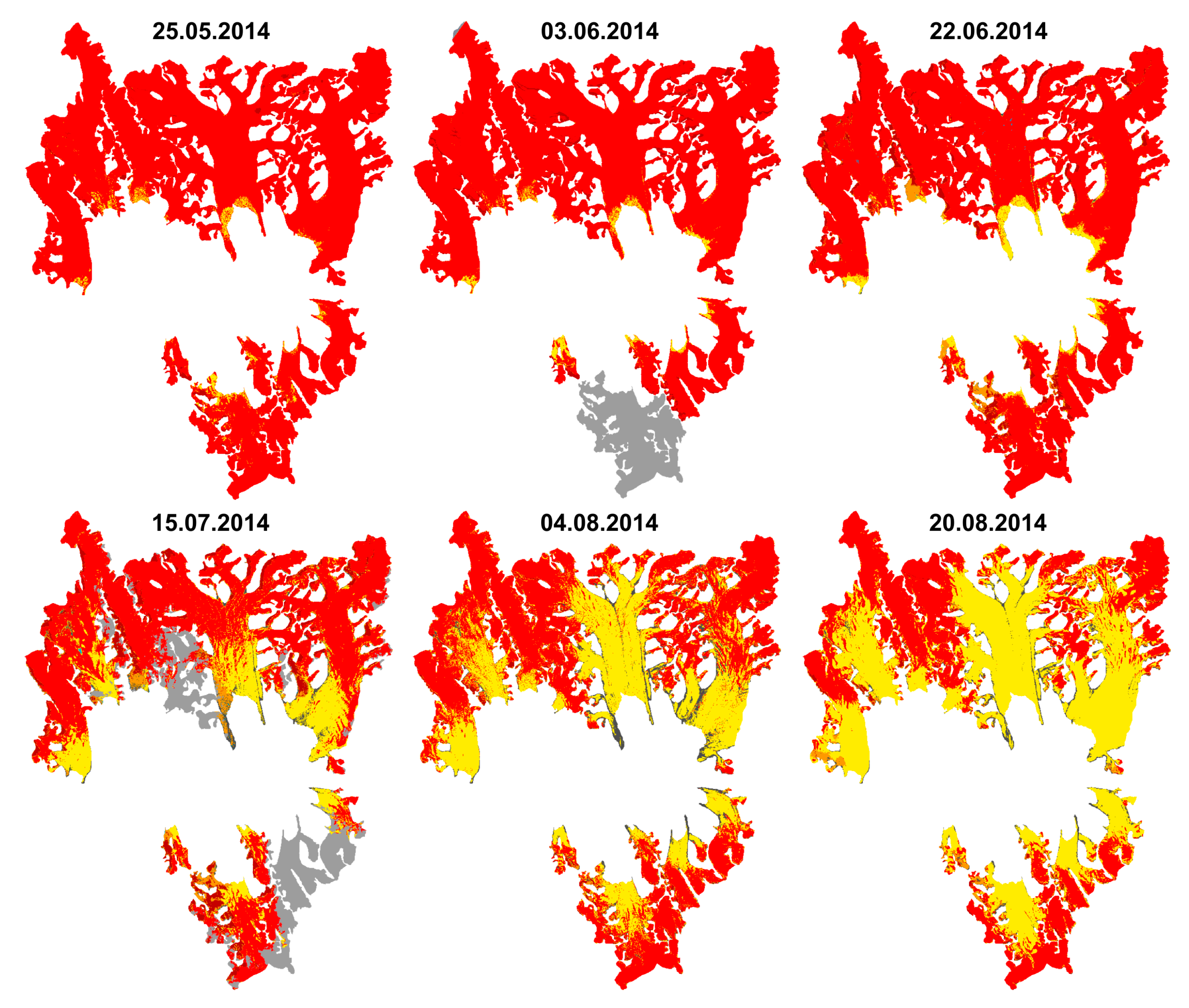
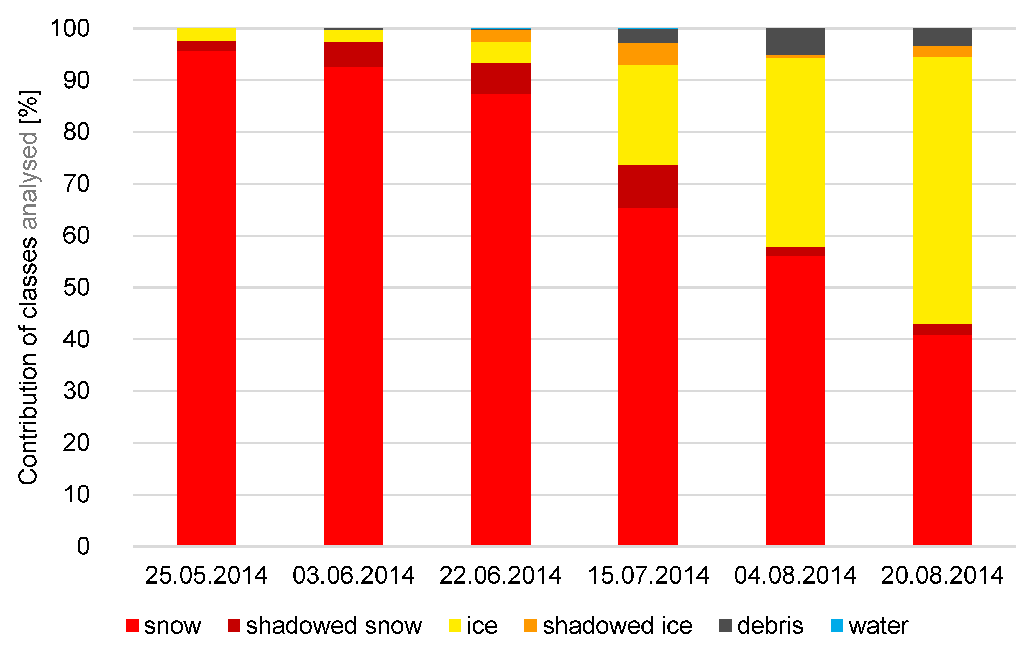
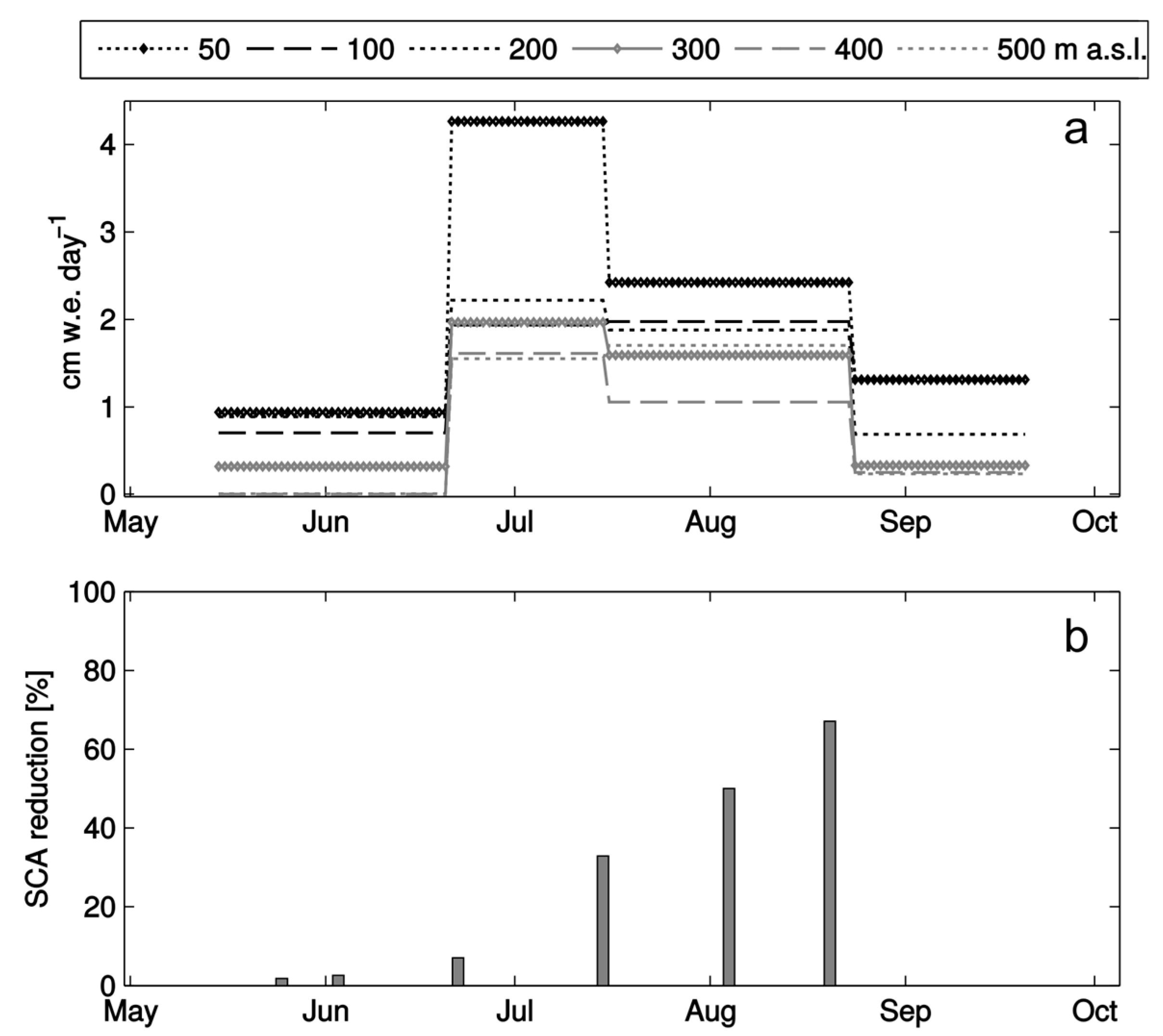
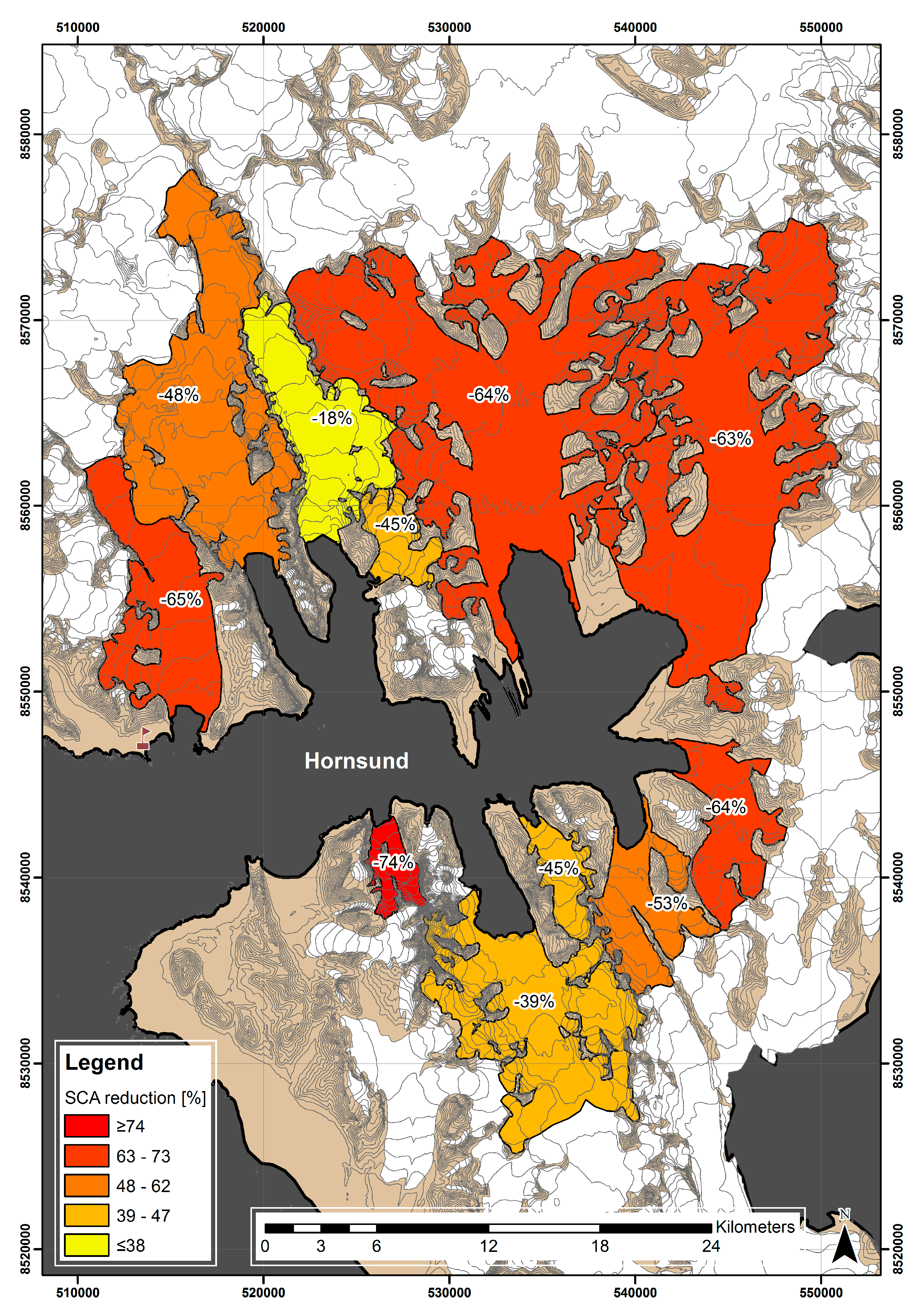
4.2. Snow Cover Melting Characteristics of Hornsund Glaciers Based on Satellite Data
5. Discussion
6. Conclusions
Acknowledgments
Author Contributions
Conflicts of Interest
References
- Jonsell, U.; Hock, R.; Holmgren, B. Spatial and temporal variations in albedo on Storglaciären, Sweden. J. Glaciol. 2003, 49, 59–68. [Google Scholar] [CrossRef]
- Stocker, T.F.; Qin, D.; Plattner, G.-K.; Tignor, M.; Allen, S.K.; Boschung, J.; Nauels, A.; Xia, Y.; Bex, V.; Midgley, P.M. Climate Change 2013: The Physical Science Basis. Contribution of Working Group I to the Fifth Assessment Report of the Intergovernmental Panel on Climate Change (IPCC); Cambridge University: Cambridge, UK; New York, NY, USA, 2013; p. 1535. [Google Scholar]
- Zemp, M.; Gärtner-Roer, I.; Nussbaumer, S.U.; Hüsler, F.; Machguth, H.; Mölg, N.; Paul, F.; Hoelzle, M. Global Glacier Change Bulletin No. 1 (2012–2013); ICSU (WDS)/IUGG (IACS)/UNEP/UNESCO/WMO: Zürich, Switzerland, 2015; p. 230. [Google Scholar]
- Hanna, E.; Huybrechts, P.; Steffen, K.; Cappelen, J.; Huff, R.; Shuman, C.; Irvine-Fynn, T.; Wise, S.; Griffiths, M. Increased Runoff from Melt from the Greenland Ice Sheet: A Response to Global Warming. J. Clim. 2008, 21, 331–341. [Google Scholar] [CrossRef] [Green Version]
- Harper, J.; Humphrey, N.; Pfeffer, W.T.; Brown, J.; Fettweis, X. Greenland ice-sheet contribution to sea-level rise buffered by meltwater storage in firn. Nature 2012, 491, 240–243. [Google Scholar] [CrossRef] [PubMed]
- Dowdeswell, J.A.; Hagen, J.O. Arctic ice caps and glaciers. In Mass Balance of the Cryosphere: Observations and Modelling of Contemporary and Future Changes; Payne, A.J., Bamber, J.L., Eds.; Cambridge University Press: Cambridge, UK, 2004; pp. 527–558. [Google Scholar]
- Shepherd, A.; Ivins, E.R.; Geruo, A.; Barletta, V.R.; Bentley, M.J.; Bettadpur, S.; Briggs, K.H.; Bromwich, D.H.; Forsberg, R.; Galin, N.; et al. A reconciled estimate of ice-sheet mass balance. Science 2012, 338, 1183–1189. [Google Scholar] [CrossRef] [PubMed]
- Błaszczyk, M.; Jania, J.A.; Kolondra, L. Fluctuations of tidewater glaciers in Hornsund Fjord (southern Svalbard) since the beginning of the 20th century. Pol. Polar Res. 2013, 34, 327–352. [Google Scholar] [CrossRef]
- Lang, C.; Fettweis, X.; Erpicum, M. Stable climate and surface mass balance in Svalbard over 1979–2013 despite the arctic warming. Cryosphere 2015, 9, 83–101. [Google Scholar] [CrossRef]
- Aas, K.S.; Dunse, T.; Collier, E.; Schuler, T.V.; Berntsen, T.K.; Kohler, J.; Luks, B. The climatic mass balance of Svalbard glaciers: A 10-year simulation with a coupled atmosphere-glacier mass balance model. Cryosphere 2016, 10, 1089–1104. [Google Scholar] [CrossRef]
- Østby, T.I.; Schuler, T.V.; Hagen, J.O.; Hock, R.; Kohler, J.; Reijmer, C.H. Diagnosing the decline in climatic mass balance of glaciers in Svalbard over 1957–2014. Cryosphere 2017, 11, 191–215. [Google Scholar] [CrossRef]
- König, M.; Winther, J.-G.; Isaksson, E. Measuring snow and glacier ice properties from satellite. Rev. Geophys. 2001, 39, 1–27. [Google Scholar] [CrossRef]
- Nolin, A.W. Recent advances in remote sensing of seasonal snow. J. Glaciol. 2010, 56, 1141–1150. [Google Scholar] [CrossRef]
- Jania, J. Dynamiczne Procesy Glacjalne na Południowym Spitsbergenie (w Świetle Badań Fotointerpretacyjnych i Fotogrametrycznych) [Dynamic Glacial Processes in South Spitsbergen (in the Light of Photointerpretation and Photogrammetric Research)]. Habilitation Thesis, University of Silesia, Katowice, Poland, 1988. [Google Scholar]
- Greuell, W.; Kohler, J.; Obleitner, F.; Głowacki, P.; Melvold, K.; Bernsen, E.; Oerlemans, J. Assessment of interannual variations in the surface mass balance of 18 Svalbard glaciers from the Moderate Resolution Imaging Spectroradiometer/Terra albedo product. J. Geophys. Res. Atmos. 2007, 112, D07105. [Google Scholar] [CrossRef]
- Moholdt, G.; Nuth, C.; Hagen, J.O.; Kohler, J. Recent elevation changes of Svalbard glaciers derived from icesat laser altimetry. Remote Sens. Environ. 2010, 114, 2756–2767. [Google Scholar] [CrossRef]
- Nuth, C.; Moholdt, G.; Kohler, J.; Hagen, J.O.; Kääb, A. Svalbard glacier elevation changes and contribution to sea level rise. J. Geophys. Res. Earth Surf. 2010, 115, F01008. [Google Scholar] [CrossRef]
- Hagen, J.O.; Olav, L.; Roland, E.; Jørgensen, T. Glacier Atlas of Svalbard and Jan Mayen; Norsk Polarinstitutt: Oslo, Norway, 1993; p. 141. [Google Scholar]
- Błaszczyk, M.; Jania, J.; Hagen, J.O. Tidewater glaciers of Svalbard: Recent changes and estimates of calving fluxes. Pol. Polar Res. 2009, 30, 85–142. [Google Scholar]
- Nuth, C.; Kohler, J.; König, M.; von Deschwanden, A.; Hagen, J.O.; Kääb, A.; Moholdt, G.; Pettersson, R. Decadal changes from a multi-temporal glacier inventory of Svalbard. Cryosphere 2013, 7, 1603–1621. [Google Scholar] [CrossRef] [Green Version]
- Muckenhuber, S.; Nilsen, F.; Korosov, A.; Sandven, S. Sea ice cover in Isfjorden and Hornsund, Svalbard (2000–2014) from remote sensing data. Cryosphere 2016, 10, 149–158. [Google Scholar] [CrossRef]
- Baranowski, S. The Subpolar Glaciers of Spitsbergen Seen Against the Climate of This Region; No. 410; Acta Universitatis Wratislaviensis: Wrocław, Poland, 1977; p. 93. [Google Scholar]
- Głowicki, B. Snow and firn patches between Hornsund and Werenskiold Glacier. Acta Univ. Wratislav. 1975, 251, 139–146. [Google Scholar]
- Laska, M.; Luks, B.; Budzik, T. Influence of snowpack internal structure on snow metamorphism and melting intensity on Hansbreen, Svalbard. Pol. Polar Res. 2016, 37, 193–218. [Google Scholar] [CrossRef]
- Migała, K.; Piwowar, B.A.; Puczko, D. A meteorological study of the ablation process on Hans Glacier, SW Spitsbergen. Pol. Polar Res. 2006, 27, 243–258. [Google Scholar]
- Szafraniec, J. Influence of positive degree-days and sunshine duration on the surface ablation of Hansbreen, Spitsbergen glacier. Pol. Polar Res. 2002, 23, 227–240. [Google Scholar]
- Marsz, A.A.; Styszyńska, A. Climate and Climate Change at Hornsund, Svalbard; Gdynia Maritime University: Gdynia, Poland, 2013. [Google Scholar]
- Marsz, A.A. Air temperature. In Climate and Climate Change at Hornsund, Svalbard; Marsz, A.A., Styszyńska, A., Eds.; Gdynia Maritime University: Gdynia, Poland, 2013; pp. 145–187. [Google Scholar]
- Łupikasza, E. Atmospheric precipitation. In Climate and Climate Change at Hornsund, Svalbard; Marsz, A.A., Styszyńska, A., Eds.; Gdynia Maritime University: Gdynia, Poland, 2013; pp. 199–211. [Google Scholar]
- Laska, M.; Grabiec, M.; Ignatiuk, D.; Budzik, T. Snow deposition patterns on southern Spitsbergen glaciers, Svalbard, in relation to recent meteorological conditions and local topography. Geogr. Ann. Ser. A Phys. Geogr. 2017, 99, 262–287. [Google Scholar]
- Grabiec, M.; Jania, J.; Puczko, D.; Kolondra, L.; Budzik, T. Surface and bed morphology of Hansbreen, a tidewater glacier in Spitsbergen. Pol. Polar Res. 2012, 33, 111–138. [Google Scholar] [CrossRef]
- Sobota, I. Snow accumulation, melt, mass loss, and the near-surface ice temperature structure of Irenebreen, Svalbard. Polar Sci. 2011, 5, 327–336. [Google Scholar] [CrossRef]
- Fierz, C.; Armstrong, R.L.; Durand, Y.; Etchevers, P.; Greene, E.; Mcclung, D.M.; Nishimura, K.; Satyawali, P.K.; Sokratov, S.A. The International Classification for Seasonal Snow on the Ground; IACS Contribution No. 1; UNESCO-IHP: Paris, France, 2009; p. 90. [Google Scholar]
- Department of the Interior U.S. Geological Survey. Landsat 8 (L8) Data Users Handbook; Earth Resources Observation and Science (EROS) Center: Sioux Falls, SD, USA, 2016; p. 106.
- Lillesand, T.; Kiefer, R.W.; Chipman, J. Remote Sensing and Image Interpretation, 6th ed.; John Wiley & Sons: New York, NY, USA, 2008. [Google Scholar]
- Dozier, J. Spectral signature of alpine snow cover from the Landsat Thematic Mapper. Remote Sens. Environ. 1989, 28, 9–22. [Google Scholar] [CrossRef]
- Łaszyca, E.; Perchaluk, J.; Kępski, D.; Górski, Z.; Wawrzyniak, T. Meteorological Bulletin. Spitsbergen–Hornsund. Summary of the Year 2014; Institute of Geophysics, Polish Academy of Sciences: Warsaw, Poland, 2015; p. 20. [Google Scholar]
- Cohen, J.; Ye, H.; Jones, J. Trends and variability in rain-on-snow events. Geophys. Res. Lett. 2015, 42, 7115–7122. [Google Scholar] [CrossRef]
- Hansen, B.B.; Isaksen, K.; Benestad, R.E.; Kohler, J.; Pedersen, Å.Ø.; Loe, L.E.; Coulson, S.J.; Larsen, J.O.; Varpe, Ø. Warmer and wetter winters: Characteristics and implications of an extreme weather event in the High Arctic. Environ. Res. Lett. 2014, 9, 114021. [Google Scholar] [CrossRef]
- Winther, J.G.; Bruland, O.; Sand, K.; Killingtveit, Å.; Marechal, D. Snow accumulation distribution on Spitsbergen, Svalbard, in 1997. Polar Res. 1998, 17, 155–164. [Google Scholar] [CrossRef]
- Sand, K.; Winther, J.-G.; Maréchal, D.; Bruland, O.; Melvold, K. Regional variations of snow accumulation on Spitsbergen, Svalbard, 1997–99. Hydrol. Res. 2003, 34, 17–32. [Google Scholar]
- Shen, Y.; Wang, Y.; Lv, H.; Qian, J. Removal of thin clouds in Landsat-8 OLI data with independent component analysis. Remote Sens. 2015, 7, 11481–11500. [Google Scholar] [CrossRef]
- Xu, M.; Jia, X.; Pickering, M. Automatic cloud removal for Landsat 8 OLI images using cirrus band. In Proceedings of the 2014 IEEE Geoscience and Remote Sensing Symposium, Quebec City, QC, Canada, 13–18 July 2014; pp. 2511–2514. [Google Scholar]
- Cohen, J. A coefficient of agreement for nominal scales. Educ. Psychol. Meas. 1960, 20, 37–46. [Google Scholar] [CrossRef]
- Nordli, Ø.; Przybylak, R.; Ogilvie, A.E.J.; Isaksen, K. Long-term temperature trends and variability on Spitsbergen: The extended Svalbard Airport temperature series, 1898–2012. Polar Res. 2014, 33, 21349. [Google Scholar] [CrossRef]
- McBean, G.; Alekseev, G.; Førland, E.J.; Fyfe, J.; Groisman, P.Y.; King, R.; Melling, H.; Vose, R.; Whitfield, P.H. Arctic Climate: Past and Present; Cambridge University: Cambridge, UK, 2005; pp. 21–60. [Google Scholar]
- Vikhamar-Schuler, D.; Isaksen, K.; Haugen, J.E.; Tømmervik, H.; Luks, B.; Schuler, T.V.; Bjerke, J.W. Changes in winter warming events in the Nordic Arctic region. J. Clim. 2016, 29, 6223–6244. [Google Scholar] [CrossRef]
- Forbes, B.C.; Kumpula, T.; Meschtyb, N.; Laptander, R.; Macias-Fauria, M.; Zetterberg, P.; Verdonen, M.; Skarin, A.; Kim, K.-Y.; Boisvert, L.N.; et al. Sea ice, rain-on-snow and tundra reindeer nomadism in Arctic Russia. Biol. Lett. 2016, 12. [Google Scholar] [CrossRef] [PubMed]
- Leszkiewicz, J.; Pulina, M. Snowfall phases in analysis of a snow cover in Hornsund, Spitsbergen. Pol. Polar Res. 1999, 20, 3–24. [Google Scholar]
- Seidel, D.J.; Ao, C.O.; Li, K. Estimating climatological planetary boundary layer heights from radiosonde observations: Comparison of methods and uncertainty analysis. J. Geophys. Res. 2010, 115, D16113. [Google Scholar] [CrossRef]
- Zhang, Y.; Seidel, D.J.; Golaz, J.-C.; Deser, C.; Tomas, R.A. Climatological characteristics of Arctic and Antarctic surface-based inversions. J. Clim. 2011, 24, 5167–5186. [Google Scholar] [CrossRef]
- Devasthale, A.; Willén, U.; Karlsson, K.G.; Jones, C.G. Quantifying the clear-sky temperature inversion frequency and strength over the Arctic Ocean during summer and winter seasons from airs profiles. Atmos. Chem. Phys. 2010, 10, 5565–5572. [Google Scholar] [CrossRef] [Green Version]
- Chutko, K.J.; Lamoureux, S.F. The influence of low-level thermal inversions on estimated melt-season characteristics in the central Canadian Arctic. Int. J. Climatol. 2009, 29, 259–268. [Google Scholar] [CrossRef]
- Grabiec, M. Stan I Współczesne Zmiany Systemów Lodowcowych Svalbardu, Południowego Spitsbergenu w Świetle Badań Metodami Radarowymi [The State and Contemporary Changes of Glacial Systems in Svalbard, Southern Spitsbergen in the Light of Radar Methods]. Habilitation Thesis, University of Silesia, Katowice, Poland, 2017. [Google Scholar]
- Benn, D.I.; Evans, D.J.A. Glaciers and Glaciation, 2nd ed.; Hodder Education: London, UK, 2010. [Google Scholar]
- Ziaja, W. Glacial recession in Sørkappland and central Nordenskiöldland, Spitsbergen, Svalbard, during the 20th century. Arct. Antarct. Alp. Res. 2001, 33, 36–41. [Google Scholar] [CrossRef]
- Uszczyk, A.; Grabiec, M.; Laska, M.; Jania, J.; Kuhn, M.; Ignatiuk, D.; Pętlicki, M.; Budzik, T. Distributed water equivalent of snowmelt in an exceptionally warm year on Hansbreen, Svalbard. Pol. Polar Res. In review.
- Kääb, A. Glacier volume changes using ASTER satellite stereo and ICESat GLAS laser altimetry. A test study on Edgeøya, Eastern Svalbard. IEEE Trans. Geosci. Remote Sens. 2008, 46, 2823–2830. [Google Scholar] [CrossRef]
- Moholdt, G.; Hagen, J.O.; Eiken, T.; Schuler, T.V. Geometric changes and mass balance of the Austfonna ice cap, Svalbard. Cryosphere 2010, 4, 21–34. [Google Scholar] [CrossRef] [Green Version]
- Hall, D.K.; Riggs, G.A.; Salomonson, V.V. Development of methods for mapping global snow cover using Moderate Resolution Imaging Spectroradiometer data. Remote Sens. Environ. 1995, 54, 127–140. [Google Scholar] [CrossRef]
- Keshri, A.K.; Shukla, A.; Gupta, R.P. ASTER ratio indices for supraglacial terrain mapping. Int. J. Remote Sens. 2009, 30, 519–524. [Google Scholar] [CrossRef]
- Xiao, X.; Shen, Z.; Qin, X. Assessing the potential of vegetation sensor data for mapping snow and ice cover: A Normalized Difference Snow and Ice Index. Int. J. Remote Sens. 2001, 22, 2479–2487. [Google Scholar] [CrossRef]
- Man, Q.X.; Guo, H.D.; Liu, G.; Dong, P.L. Comparison of different methods for monitoring glacier changes observed by Landsat images. IOP Conf. Ser. Earth Environ. Sci. 2014, 17, 012127. [Google Scholar] [CrossRef]


| ID A | Glacier | Aspect A | Area B | Length B km | Mean Elevation B | ELA C | ||
|---|---|---|---|---|---|---|---|---|
| AC | AB | km2 | Glacier | Terminus | m | m | ||
| 124 04 | Körberbreen | N | N | 9.4 | 5.3 | 1.24 | 317 | – |
| 124 07 | Samarinbreen | NW | NW | 84.0 | 10.6 | 3.96 | 333 | 352 |
| 124 08 | Chomjakovbreen | N | NW | 13.1 | 7.0 | 1.48 | 313 | 318 |
| 124 09 | Mendelejevbreen | NE | N | 31.1 | 9.2 | 3.57 | 222 | 231 |
| 124 10 | Svalisbreen | N | W | 31.3 | 10.2 | 2.28 | 232 | 318 |
| 124 11 | Hornbreen | S | SW | 176.2 | 25.5 | 5.47 | 289 | 398 |
| 124 12 | Storbreen | S | S | 196.5 | 21.7 | 6.89 | 287 | 383 |
| 124 16 | Kvalfangarbreen | SW | SW | 13.5 | 5.2 | 0.63 | 277 | 331 |
| 124 17 | Mühlbacherbreen | S | S | 51.6 | 14.05 | 1.82 | 376 | 373 |
| 124 18 | Paierlbreen | SE | SE | 106.1 | 22.0 | 2.15 | 370 | 400 |
| 124 20 | Hansbreen | SE | S | 53.9 | 15.37 | 1.99 | 291 | 342 |
| Month | Hornsund | Hansbreen H4 | Hansbreen H6 | Hansbreen H9 | ||||
|---|---|---|---|---|---|---|---|---|
| Days | Sum | Days | Sum | Days | Sum | Days | Sum | |
| January | 5 | 3.2 | 1 | 0.4 | – | – | 0 | 0.0 |
| February | 12 | 13.5 | 4 | 4.1 | – | – | 0 | 0.0 |
| March | 3 | 2.0 | 0 | 0.0 | – | – | 0 | 0.0 |
| April | 0 | 0.0 | 0 | 0.0 | 0 | 0.0 | 0 | 0.0 |
| May | 13 | 16.5 | 6 | 5.8 | 3 | 2.2 | 2 | 0.9 |
| June | 30 | 98.7 | 21 | 35.2 | 19 | 27.1 | 15 | 18.3 |
| July | 31 | 172.9 | 31 | 74.6 | 31 | 78.8 | 31 | 77.4 |
| August | 31 | 154.8 | 31 | 70.8 | 31 | 58.8 | 28 | 48.3 |
| September | 25 | 74.4 | 19 | 28.1 | 13 | 16.8 | 8 | 12.4 |
| October | 14 | 41.4 | 12 | 23.7 | 9 | 17.8 | 6 | 7.0 |
| November | 5 | 8.0 | 5 | 3.4 | 2 | 1.5 | 1 | 0.0 |
| December | 1 | 0.0 | 0 | 0.0 | 0 | 0.0 | 0 | 0.0 |
| Year | 170 | 585.4 | 130 | 246.1 | 108 | 203.0 | 91 | 164.3 |
| Glacier | Site | Elevation | Snow Depth | Bulk Density | SWE | IF | MFcr |
|---|---|---|---|---|---|---|---|
| m a.s.l. | m | kg m−3 | m w.e. | % | % | ||
| Flatbreen | F1 | 198 | 1.67 | 397 | 0.66 ± 0.08 | – | – |
| F2 | 284 | 2.72 | 417 | 1.13 ± 0.14 | – | – | |
| F3 | 380 | 3.84 | 430 | 1.65 ± 0.19 | – | – | |
| Hansbreen | H4 | 187 | 1.60 | 374 | 0.60 ± 0.08 | 2.2 | 25.0 |
| H6 | 278 | 2.10 | 399 | 0.84 ± 0.11 | 4.8 | 15.5 | |
| H9 | 424 | 2.78 | 466 | 1.30 ± 0.14 | 5.0 | 7.9 | |
| Storbreen | S1 | 166 | 1.46 | 376 | 0.55 ± 0.07 | – | – |
| S2 | 266 | 1.63 | 367 | 0.60 ± 0.08 | – | – | |
| S3 | 425 | 2.59 | 404 | 1.05 ± 0.13 | – | – |
| No. | Imagery ID | Date | Cloud Cover [%] | Sun Elevation [°] | Kappa Coefficient | Overall Accuracy |
|---|---|---|---|---|---|---|
| 1 | LC82090052014145LGN00 | 25 May 2014 | 7.55 | 33.67 | 0.99458 | 99.46 |
| 2 | LC82080052014154LGN00 | 3 June 2014 | 26.92 | 35.04 | 0.97803 | 97.88 |
| 3 | LC80282392014173LGN00 | 22 June 2014 | 47.85 | 17.69 | 0.99436 | 99.43 |
| 4 | LC80292392014196LGN00 | 15 July 2014 | 10.95 | 15.94 | 0.99529 | 99.53 |
| 5 | LC82100052014216LGN00 | 4 August 2014 | 20.31 | 29.99 | 0.96057 | 95.95 |
| 6 | LC82100052014232LGN00 | 20 August 2014 | 44.05 | 25.16 | 0.99790 | 99.80 |
© 2017 by the authors. Licensee MDPI, Basel, Switzerland. This article is an open access article distributed under the terms and conditions of the Creative Commons Attribution (CC BY) license (http://creativecommons.org/licenses/by/4.0/).
Share and Cite
Laska, M.; Barzycka, B.; Luks, B. Melting Characteristics of Snow Cover on Tidewater Glaciers in Hornsund Fjord, Svalbard. Water 2017, 9, 804. https://doi.org/10.3390/w9100804
Laska M, Barzycka B, Luks B. Melting Characteristics of Snow Cover on Tidewater Glaciers in Hornsund Fjord, Svalbard. Water. 2017; 9(10):804. https://doi.org/10.3390/w9100804
Chicago/Turabian StyleLaska, Michał, Barbara Barzycka, and Bartłomiej Luks. 2017. "Melting Characteristics of Snow Cover on Tidewater Glaciers in Hornsund Fjord, Svalbard" Water 9, no. 10: 804. https://doi.org/10.3390/w9100804
APA StyleLaska, M., Barzycka, B., & Luks, B. (2017). Melting Characteristics of Snow Cover on Tidewater Glaciers in Hornsund Fjord, Svalbard. Water, 9(10), 804. https://doi.org/10.3390/w9100804