Article

An Integrated Modelling System to Predict Hydrological Processes under Climate and Land-Use/Cover Change Scenarios

1
Department of Geomatics Engineering, University of Calgary, 2500 University Drive NW, Calgary, AB T2N 1N4, Canada
2
Alberta Environment and Parks, Calgary, AB T2N 1N4, Canada
3
Department of Civil and Geological Engineering, Global Institute for Water Security, School of Environment and Sustainability, University of Saskatchewan, Saskatoon, SK S7N 5E8, Canada
4
Earth and Atmospheric Sciences, University of Alberta, 116 St. and 85 Ave., Edmonton, AB T6G 2R3, Canada
*
Author to whom correspondence should be addressed.
Water 2017, 9(10), 767; https://doi.org/10.3390/w9100767
Submission received: 30 June 2017 / Revised: 27 September 2017 / Accepted: 29 September 2017 / Published: 9 October 2017

Abstract

:
This study proposes an integrated modeling system consisting of the physically-based MIKE SHE/MIKE 11 model, a cellular automata model, and general circulation models (GCMs) scenarios to investigate the independent and combined effects of future climate and land-use/land-cover (LULC) changes on the hydrology of a river system. The integrated modelling system is applied to the Elbow River watershed in southern Alberta, Canada in conjunction with extreme GCM scenarios and two LULC change scenarios in the 2020s and 2050s. Results reveal that LULC change substantially modifies the river flow regime in the east sub-catchment, where rapid urbanization is occurring. It is also shown that the change in LULC causes an increase in peak flows in both the 2020s and 2050s. The impacts of climate and LULC change on streamflow are positively correlated in winter and spring, which intensifies their influence and leads to a significant rise in streamflow, and, subsequently, increases the vulnerability of the watershed to spring floods. This study highlights the importance of using an integrated modeling approach to investigate both the independent and combined impacts of climate and LULC changes on the future of hydrology to improve our understanding of how watersheds will respond to climate and LULC changes.

1. Introduction

Climate and land-use/land-cover (LULC) changes are two inter-related factors that can directly and indirectly alter the hydrologic system and subsequently the sources of water supply [1,2,3]. However, the responses of hydrological processes to climate and LULC change have been often investigated separately. For instance, there have been studies to investigate how changes in LULC can influence hydrological regimes through modifications of the infiltration rates [4], evapotranspiration losses [5], and both the peak runoff and the total runoff volume [6]. On the other hand, there have been studies that predicted how climate change can alter the timing of high flows [7,8,9,10], and modify the frequency and magnitude of extreme events, such as floods and droughts (e.g., [11,12]). Numerous studies have been conducted to investigate hydrological responses to future climate change scenarios (e.g., [13,14,15]). Climate models, downscaling techniques, and hydrological models are the building blocks that are used in serial order for climate impact assessment [16,17,18,19,20]. The output of each of them is associated with uncertainty, and the cascade of uncertainty from climate models to hydrological impacts often results in excessive uncertainty, often referred to as “deep uncertainty”. Many attempts have been made to reduce the uncertainties related to this cascade (for detail, see [21,22,23,24]) by employing higher resolution GCMs (e.g., [25]), advanced downscaling approaches (e.g., [26]) and physically-based distributed hydrological models (e.g., [9]). However, less attention has been given to incorporate the dynamics of land surface changes into the modelling framework for climate change impact assessment [27]. Farjad et al. [9] investigated impact of climate change on hydrology using a physically-based distributed model while considering different LULC maps, corresponding to different climate time intervals, for calibration and validation of the model. They indicated that physically-based fully distributed models reduce the uncertainty linked to calibration compared to lumped models which are climate sequence dependent, especially when the dynamics of the land surface is used for the calibration procedure. However, the study did not consider the changes in the physical properties of the land surface in the simulation of future hydrological processes. This in return can introduce uncertainty in the model outcomes, especially for long-term climate change impact.
Other studies have focused on the impact of LULC change on hydrology (e.g., [28,29]). Changes in LULC patterns, obtained from either LULC change modeling or hypothetical scenarios, are incorporated into hydrological models. These models range from simple rainfall–runoff models such as those based on unit hydrographs [30] that provide limited information on the relationship between LULC patterns and hydrological components [31], to distributed physically based models such as MIKE SHE [32] that represent the spatial variability of the surface and subsurface along with their interactions in a watershed [29]. For instance, Wijesekara et al. [29] employed a distributed physically based MIKE SHE/MIKE 11 model to investigate the response of hydrological processes to four scenarios of LULC change while assuming the climate remains stationary. Such assumptions conflict with the inherent complex interaction of the system components. Hendriks [33] showed that a change from forest to grassland can affect evapotranspiration (ET) differently according as a function of climate condition. In a dry climate, a conversion from forest to grassland caused a significant increase in ET while it did not increase ET in wet climate conditions. This is because the aerodynamic resistance and surface resistance respond differently to various climatic conditions.
An evaluation of change in a hydrological regime based solely on either climate or LULC change may not provide a reliable conclusion since the hydrological regime is simultaneously tied to these two controlling factors and their interaction. A clear understanding of hydrological processes can be difficult to ascertain from LULC or climate change alone when a complex dynamical and physical interaction exists between those components [34]. Therefore, there is a need for an integrated modeling system to investigate the independent and combined effects of future climate and LULC changes on hydrology. To date, a limited number of such integrated systems have been developed and they often have limitations in the way they address the complexity of some major physical processes. For instance, Tu [35] and Antonellini et al. [36] employed a lumped, conceptual hydrological model to simulate hydrological processes under climate and LULC change. However, a lumped, conceptual hydrological model that has been calibrated to current climate conditions might be inadequate for application in a climate change context, compared to physically based models [9,37]. Khoi and Suetsugi [38] employed the semi-distributed SWAT model to evaluate the responses of hydrological processes to climate and LULC change in the Be River Catchment, in Vietnam. The SWAT model uses empirical equations that were developed for the US climate conditions, which may not be suitable when applied in different climates. In addition, groundwater components and their interactions with surface water are not included in the model. Montenegro and Ragab [39] used the physically based distributed DiCaSM model to assess the combined impact of climate and LULC in the Ipanema catchment in Brazil. However, they calibrated and validated the model based on constant LULC conditions and changing climate rather than applying different LULC maps corresponding to different climate time intervals specified for the model simulation periods.
Other limitations are associated with the way LULC changes are predicted. The Intergovernmental Panel on Climate Change (IPCC) has not provided sufficient information related to future land-use change corresponding to climate scenarios, which makes linking global and local scale for land-use projection difficult [40,41,42]. Although a few efforts have been undertaken to downscale land use from coarse scales to finer scales based on IPCC’s Special Report on Emissions Scenarios (SRES) [42,43,44], they have been limited to either downscaling from global scale to continental scale [45,46] or to sub-continental scale, which only provides a narrow range of land-use types [47]. To overcome the challenges that constrain the connection of global scale and local scale land-use projection, there is a need to predict future LULC change at the local scale either independent from IPCC-SRES or corresponding to each climate change scenario while taking to account the local regulations in a region. This approach not only overcomes the uncertainty related to downscaling from global scale to local scale, but also allows a user to take into account the local regulations and plans of future land development in a region. A number of studies have used LULC modeling to predict future LULC change at the local scale independent from IPCC-SRES. These studies have however generated only one LULC map for a specific year and utilized for long-term climate change study [48,49]. This may result in missing important LULC events and processes that likely influence hydrological processes over a long-term simulated period. An integrated modeling system requires a rigorous LULC prediction method to replicate spatial patterns and real-world dynamics. Prediction of LULC changes should be done at different time intervals in a spatially explicit context, especially for long-term climate and LULC impact assessment in an urban watershed.
Similarly, some authors [48] employed hypothetical values to define future climate conditions rather than using GCMs, which are required to adequately represent the physical processes in the atmosphere, ocean, land surface, and cryosphere, along with the geophysical climate feedbacks (changes in water vapour, clouds, and sea ice albedo) and the biogeochemical feedbacks (changes in sources of greenhouse gases and vegetation albedo). Other authors employed only one or two random GCM scenarios [35,36,39] due to computationally intensive simulation especially when the combined and independent impacts of climate and LULC change need to be distinguished.
Addressing the limitations of the previous studies in capturing the dynamical, physical, and distributed nature of hydrological processes in response to both climate and LULC changes, this research proposes a comprehensive integrated modeling system, which consists of three major components: a LULC change cellular automata (CA) model, the distributed physically-based, MIKE SHE/MIKE 11 model, and GCM scenarios. Our in-house CA allows the prediction of LULC changes at different time intervals, corresponding to climate change scenarios, and makes it highly compatible with the intervals of hydrological simulations. In addition, the rule-based nature of the CA enables the consideration of external (e.g., socio-economical) and internal (e.g., distance from river, distance to city center) driving factors, and capable of simulating a range of LULC change scenarios corresponding to each climate change scenario while taking to account the local regulations in a region. In addition, the spatially explicit CA model provides detailed spatial characteristics of the land surface, which are required in MIKE SHE/MIKE 11 which is based on physical principles and considers a catchment as finite geo-referenced computational units with different responses to forcing inputs. The modeling system is applied to the Elbow River watershed in southern Alberta, Canada to understand how hydrological processes respond to both LULC and climate change.

2. Case Study and Method

2.1. The Elbow River Watershed

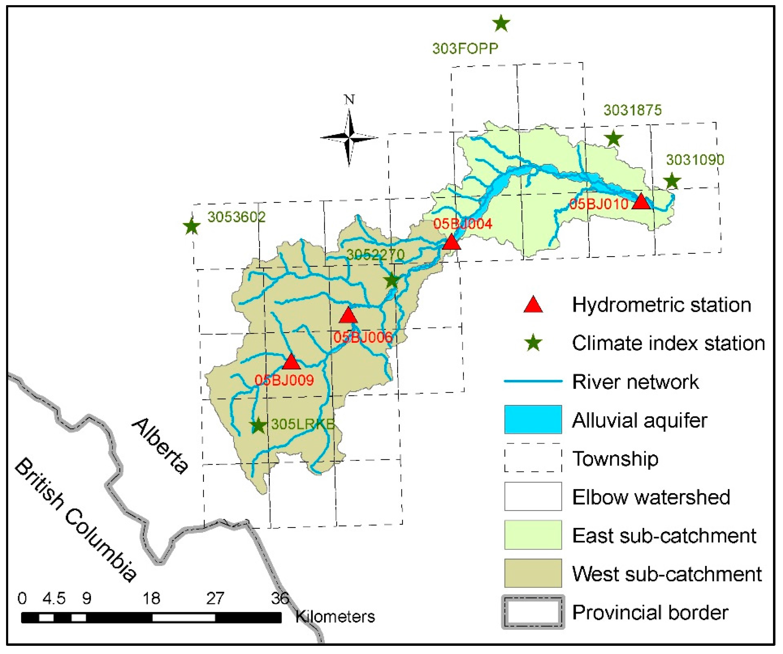
The Elbow River watershed (Figure 1) lies between 50°30′ and 51°20′ north latitude and 114°00′ and 115°00′ west longitude with a drainage area of 1235 km2. The watershed is a snow-dominated watershed with snow and ice accumulating during the winter. Warming temperature results in an increase in river discharge during spring and early summer, and a combination of snowmelt and high level of rainfall (typically) in June generates the highest flows of the river. The river originates in the eastern slopes of the Rocky Mountains and flows eastward, before entering the Glenmore reservoir and the Bow River in the City of Calgary. Elevations of the watershed range from a high of over 3000 m above sea level to a low of 1080 m. The watershed is characterized by a complex hydrological regime due to variations in climate, geomorphology, and topography in the west and east sub-catchments, along with complex surface and groundwater interactions along the river [8,9]. To take these variations into consideration, the watershed was delineated into west and east sub-catchments. The west and east sub-catchments are upstream and downstream of the 05BJ004 station (Bragg Creek), respectively (Appendix A). In addition, the hydrology of the watershed is influenced by heterogeneous LULC that includes evergreen forest (34%), agricultural land (16.7%), deciduous forest (10%), rangeland/parkland (6.2%), urban area (5.9%), and forest clear-cut (1.8%) [29].
Long-term historical climate data (1961–2005), obtained from Alberta Environment and Parks (AEP), indicate that the mean annual temperature is 2.5 °C with the warmest month being July (13.2 °C) and the coldest month being January (−9 °C) for the watershed. The mean annual precipitation is 690 mm with a high spatial variability due to the large differences in elevation. The largest amount of precipitation occurs in June (99.6 mm) (location of the climate stations is provided in (Appendix A and Appendix B). The mean annual discharge varies from a low of 3.33 m3/s at the 05BJ009 hydrometric station in the front ranges of the Rocky Mountains in the west sub-catchment to a high of 10 m3/s at the 05BJ010 station upstream of the outlet of the watershed (Figure 1). Historical data indicate that a large portion of the average annual discharge (~93%) is generated at the 05BJ004 station, considering 100% of discharge at the 05J010 station.
The hydrology and ecosystem balance of the watershed are under pressure due to the rapid population growth and land development in the east portion of the watershed, included and adjacent to the City of Calgary. The population of Calgary has increased by 71% between 1985 and 2010 (The City of Calgary, 2010), and is expected to rise on average by 1.6% annually in the next 25 years [50]. The watershed has experienced several droughts [51] and floods over the past decades (The City of Calgary, 2013). It is therefore critical to understand the future possible responses of the hydrological processes to changes in climate and LULC since they can induce considerable stress in addition to economic and social costs.

2.2. Methodological Framework

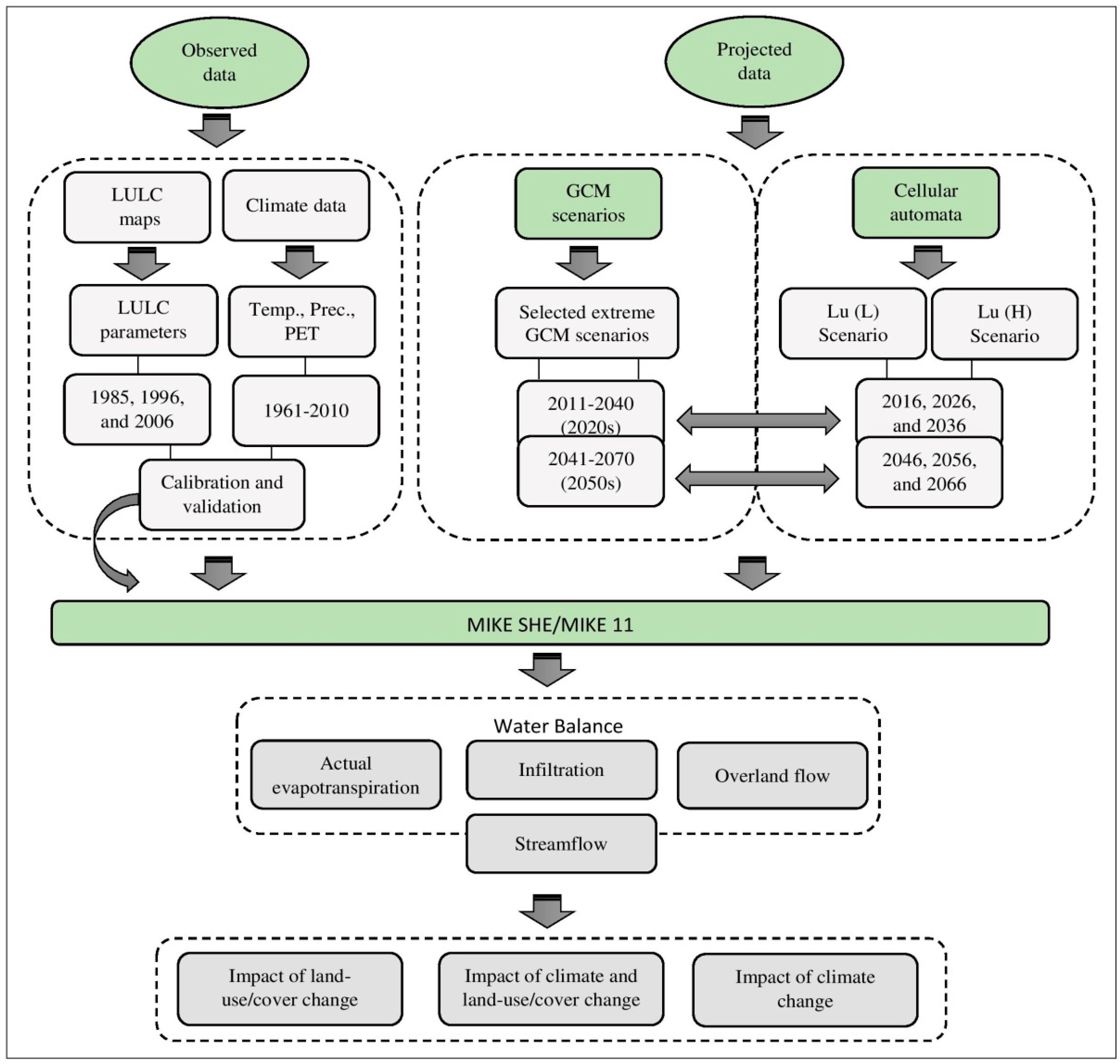
The methodological framework includes four main components: (1) gathering historical LULC and climate data; (2) GCMs-scenarios; (3) LULC change modeling with a cellular automata; and (4) hydrological modeling using MIKE SHE/MIKE 11 (Figure 2).

2.2.1. Observed Climate and LULC Data

The climate variables required by MIKE SHE/MIKE 11 are minimum and maximum air temperature, precipitation, and potential evapotranspiration (PET). These data were obtained from the Agroclimatic Atlas of Alberta for the period of 1961–2010 on a daily basis. Temperature and PET were interpolated for each township (9.6 by 9.6 km2) based on over 1200 stations within Alberta and about 1400 just beyond Alberta’s borders. The spatial distribution of precipitation over the watershed was generated based on six climate index stations based on the Thiessen polygon method using MIKE SHE/mike 11 model described in Section 2.2.4 [52]. Hydrogeological information was obtained from Alberta Environment and Parks.
Soil information was retrieved for the watershed from two databases: the Agricultural Region of Alberta Soil Inventory Database and the Canadian Soil Information Service Data sources. This information was used to create the soil layer for the MIKE SHE/MIKE 11 model. The topography layer was derived from the 80 m spatial resolution digital elevation model from GeoBase [53]. Physical land properties such as leaf area index (LAI) and root depth (RD) were derived from historical LULC maps generated from Landsat Thematic Mapper images at 30 m resolution, acquired for the years 1985, 1992, 1996, 2001, 2006, and 2010. Time series of LAI and RD were created for each LULC class based on values obtained from the literature.
Daily discharge was acquired from AEP for the period of 1961–2010 for four hydrometric stations: 05BJ009, 05BJ006, 05BJ004, and 05BJ010 (Figure 1), while (stationary) cross-section information was obtained from field surveys and LiDAR generated data. Stationary cross-section information introduces some uncertainties in hydrological modelling which is described in detail in Di and Montanari [54].

2.2.2. GCMs-Scenarios

The output of two climate models, the CGCM2 (Canadian Centre for Climate Modelling and Analysis) and the NCARPCM (National Centre for Atmospheric Research), forced by two emission scenarios, A1B [35,55] and B2 [14,56], were used (NCARPCM-A1B and CGCM2-B2) to construct time series climate variables for the periods of 2020s (2011–2040) and 2050s (2041–2070). The A1B scenario assumes a world of very rapid global economic and population growth with peaks in mid-century, whereas B2 describes lower growth rates of the global economic and population. These two GCM-scenarios—identified as extreme climate scenarios in the region—were utilized to allow for comparisons with previous studies conducted by Alberta Environment and Parks (AEP). However, in future works, the authors recommend considering multiple GCMs, either independently or in ensemble mode along with a range of climate change scenarios of the Intergovernmental Panel on Climate Change Fifth Assessment Report (IPCC AR5).
The climate variables associated with these scenarios include temperature and precipitation over two periods (2020s and 2050s) relative to 1961–1990. The widely used delta change method was utilized for downscaling climate model outputs into hydrological model inputs [17,20,57,58]. This method is easy to employ, but it has the limitation of retaining the temporal structure of the baseline data [59]. To overcome this limitation, only changes in annual and seasonal responses of hydrological processes to climate scenarios were taken into account in this study [60]. PET, another required climate variable, was calculated using the Hargreaves and Samani’s temperature-based model [61]. This model was selected using a rigorous procedure based on a comprehensive literature review and a comparison of the Hargreaves–Samani [61], Thornthwaite [62], and Blaney–Criddle [63] models against the PET rates obtained from AEP as reference.

2.2.3. LULC Change Modeling and Scenarios

An in-house developed CA model was employed to simulate future LULC change in the watershed [29]. CA allows the characterization of complex spatial systems through a bottom up simulation of local interactions between neighbouring cells. A typical CA consists of five main elements: (i) geographic domain represented by a grid of cells; (ii) cell states that define the set of possible values associated to the cells; (iii) a neighbourhood of adjacent cells that can influence the central cell; (iv) transition rules that define the next state of the central cells according to internal and external factors; and (v) discrete time step that allows all cells to change state simultaneously. This study modified the algorithm related to the last two characteristics of the CA model developed by Wijesekara et al. [29] for the purpose of climate impact assessment as follows. In order to consider the uncertainty related to long-term prediction, two opposite scenarios of LULC change, Lu-(PL) and Lu-(PH), were identified to cover a plausible range of change in the watershed. These scenarios represent alternative futures under different sets of assumptions to explore possible future developments in complex systems with high levels of uncertainty [44]. The Lu-(PL) scenario captures the possibility of lower growth in economy and immigration and consequently in population, while higher growth is projected under the Lu-(PH) scenario. The long-term projected data and information for these scenarios were obtained from the Alberta Treasury Board and Finance [50]. The LULC changes were simulated up to 2070 at a 10-year interval, thereby providing simulated LULC maps for the years 2016, 2026, 2036, 2046, 2056, and 2066. Based on a comprehensive sensitivity analysis, the four factors governing the LULC changes in the watershed were distance to Calgary city center, distance to a main road, distance to a main river, and the ground slope. The neighbourhood configuration was designed to approximate a circle around a center cell containing three concentric neighbourhood rings. The influence of neighbouring cells within each ring on the central cell was constant, but varies between rings.
Historical LULC maps for the years 1985, 1992, 1996, 2001 and 2006, which including the LULC classes water, rock, road, deciduous forest, agriculture land, rangeland/parkland, built-up areas, and clear-cut areas, were used to calibrate the CA model. The extraction of the transition rules was done as follow. First, the number of cells in each LULC class and their transitions from one state to another as observed in the historical maps were computed. Then, for each LULC transition that occurred in the past, frequency histograms were built to identify the neighbourhood configuration, state of the cells within the neighbourhood, and external driving factor that best represent the conditions associated to these transitions. These values were used to construct the transition rules. The validation was conducted through a comparison of the simulated and reference LULC map of 2010 using a set of landscape metrics. The spatial distribution of LULC selected parameters such as root depth (RD), surface roughness, and leaf area index (LAI) was created with these LULC maps and employed as inputs into the hydrological model MIKE SHE/MIKE 11.

2.2.4. Hydrological Modeling

MIKE SHE/MIKE 11 is a distributed, physically-based model that includes all the major hydrological components and their interactions such as overland flow, saturated and unsaturated flow, channel flow, and evapotranspiration. The model discretizes the watershed by horizontal-grid square networks for surface and groundwater flow components, which are connected to the unsaturated zone through vertical columns of nodes at each grid. In this study, a finite difference approximation of the St. Venant equation was used to solve channel flow. In addition, the two-layer water balance method was employed to divide the unsaturated zone (UZ) into a root zone, from which water can be taken by plants, and a zone below the root zone, where water can be recharged into the saturated zone.
Saturation zone (SZ) computations were accomplished using the 3D Darcy equation and solved using a numerical finite-difference scheme. The 3D finite difference method relates the unsaturated zone model to a dynamic water table. The saturation zone was configured using six geologic layers. For each geological layer, four hydrogeologic parameters were assigned, namely vertical hydraulic conductivity, horizontal hydraulic conductivity, specific storage, and specific yield. Actual evapotranspiration (ET) was simulated by the coupled Kristensen and Jensen model [64] and the two-layer water balance UZ/ET method [65]. This approach considers parameters that are involved in the processes of interception, plant transpiration, and soil evaporation. The parameters can be grouped into characterisation of the vegetation cover such as LAI and RD, and the physical soil properties, such as the soil moisture contents at the wilting point, field capacity, and a constant infiltration capacity. Land surface properties were extracted from LULC maps. Leaf area index (LAI) values vary from 0 to 7. Evergreen and Deciduous have a value of 5, during the full leaf period, while agriculture has a value between 2 and 4 during the summer period. During the winter months, this value drops to 0.2 for seasonal vegetation. Root depth (RD) for forest areas is usually defined with a higher root depth which is considered constant. Values for agricultural areas begin at 0, peak when the crops are fully grown, and drop down to 0 when the crops are harvested. The interception process was modeled based on an interception storage that must be filled before adding water to the soil moisture and ponded water on the ground surface. The process of soil evaporation occurs from the upper UZ layer, and also from excess soil water when the soil reaches field capacity, while transpiration only decreases the water content in the root zone (it does not occur below the root zone). On the other hand, when the plant roots reach the capillary zone, water is extracted directly from the SZ. However, this process does not reduce the soil moisture content, whereas any water deficit can be replaced by water carried from the SZ up through capillary action. In addition, an ET surface depth parameter was defined at which evapotranspiration extracts water directly from the water table if capillary zone reaches the ground surface at the defined ET surface depth.
Snowmelt was calculated based on the degree-day method using air temperature, degree-day factor (mm snow/day/°C), and threshold melting temperature (the temperature at which snow begins to melt). Therefore, if the air temperature is above the threshold temperature then the snow starts to melt; otherwise, the precipitation accumulates as snow. A temporal changing value for the degree-day coefficient parameter was obtained from the literature and was adjusted during calibration. For the melting threshold temperature in the mountainous area, a value of 0.5 °C (elevation higher than 1700 m), and for the remaining area a uniform value of 0 were used. These values were found during the calibration. Additional parameter adjustments (during calibration) included setting the minimum snow storage value to 100 mm and the maximum wet snow fraction to 0.1 (DHI Water and Environment 2010).
For the MIKE 11 model, a river network was created for the Elbow River and its tributaries with 353 cross sections, obtained from field surveys and LiDAR generated data. Furthermore, a water stage-discharge relationship was applied as the boundary condition at the downstream end of the main river stream.
A comprehensive calibration and validation procedure was conducted using the split-sample, multi-criteria, and multi-point method. The time period 1981–1991 with the LULC map of 1985 was used for calibration while the time periods of 1991–2000 and 2001–2010 with their corresponding LULC maps of 1996 and 2006 were used for validation. A comparison of simulated data against snow storage, streamflow, and groundwater level was performed, which indicated a satisfactory agreement between the simulated and observed values. Table 1 shows the model performance by comparing the simulated results with observed streamflow during calibration and validation periods for different hydrometric stations. Simulated and observed groundwater level and snow storage were compared using the mean absolute error (MAE) and the Pearson’s correlation coefficient (PC). For calibration, the average daily and monthly indices values, respectively, were 0.60 and 0.64 (MAE) and 0.82 and 0.86 (PC), whereas, for validation, the average daily and monthly indices were 0.62 and 0.66 (MAE) and 0.83 and 0.84 (PC).

2.2.5. Simulated Scenarios

To investigate changes in the water balance of the watershed, a base case scenario (BL) was defined to represent the hydrological responses to the baseline climate from 1961 to 1990 with the LULC map of 1985. Then, the water balance was calculated for the following three scenarios over different time periods, relative to the BL scenario:
(1)
Impact of LULC change on hydrological processes:
(a)
LU-H scenario: This scenario assumes constant baseline climate (1961–1990) while LULC changes for the 2020s and 2050s under the Lu-(PH) scenario.
(b)
LU-L scenario: This scenario assumes constant baseline climate (1961–1990) while LULC changes for the 2020s and 2050s under the Lu-(PL) scenario.
(2)
Impact of climate change on hydrological process:
(a)
A1B scenario: This scenario considers the A1B climate scenario while LULC is constant.
(b)
B2 scenario: This scenario considers the B2 climate scenario while LULC is constant.
(3)
Impact of climate and LULC change on hydrological processes:
(a)
LU(H)-A1B scenario: This scenario considers the A1B climate scenario with the LU-PH scenario.
(b)
LU(L)-A1B scenario: This scenario considers the A1B climate scenario with the LU-PL scenario.
(c)
LU(H)-B2 scenario: This scenario considers the B2 climate scenario with the LU-PH scenario.
(d)
LU(L)-B2 scenario: This scenario considers the B2 climate scenario with the LU-PL scenario.
The hydrological processes considered in the water balance of the watershed are evapotranspiration, infiltration, and overland flow. Ten-year intervals were considered for the simulation of hydrological processes. Climate data for three periods, namely 2011–2020, 2021–2030, and 2031–2040 with the corresponding predicted LULC maps of 2016, 2026, and 2036 were used for the simulation in the 2020s (Figure 3). For the simulation of hydrological processes in the 2050s, climate data for three periods, namely 2041–2050, 2051–2060, and 2061–2070 with the corresponding predicted LULC maps of 2046, 2056, and 2066 were used. These simulations were iterated for each individual scenario.

3. Results and Discussion

In this section, the annual and seasonal changes in climate scenarios are described, followed by the simulation results of hydrological processes in response to climate and LULC change.

3.1. Annual and Seasonal Changes in Climate Scenarios

A rise in the average annual temperature occurs for both the A1B (0.7 °C and 2.2 °C) and B2 (1.5 °C and 2.3 °C) scenarios in the 2020s and 2050s, respectively (Figure 4) (the names of the scenarios are not attached with their corresponding GCMs for simplicity and fluidity reasons). In comparison, the average annual precipitation increases for A1B (1.2% and 11.1%) and decreases for B2 (−0.4% and −2.2%) in the 2020s and 2050s, respectively (Figure 4).
The average seasonal changes in the air temperature indicate an increase for both A1B and B2 scenarios in all seasons in the 2020s and 2050s (Figure 4). Winter temperature exhibits the largest change under the A1B (0.9 °C and 2.8 °C) and B2 (2.2 °C and 3.2 °C) scenarios in the 2020s and 2050s. The seasonal rise in temperature under the A1B scenario varies in the range of 0.5–0.9% and 1.7–2.8% while it varies in the range of 0.7–2.2% and 1.4–3.2% under B2 in the 2020s and 2050s, respectively. Although these changes occur in the same direction, even a small magnitude of change in temperature with a different temporal pattern may influence hydrological components differently depending on the season. For instance, an increase in air temperature during winter, spring, and early summer may result in a rise in runoff when snow is the dominant factor in the watershed. On the other hand, an increase in air temperature during fall and late summer may result in water losses when there is a reduction in the snow storage and evapotranspiration is the dominant factor in the water balance.
The complexity of interactions between the climate and the hydrology regime in the watershed can be enhanced when precipitation and temperature tend to offset each other’s influence differently in different seasons. In other words, the dominant climate variable in a season may differ depending on the season. Changes in seasonal precipitation show that fall precipitation increases under both the A1B (5.6% and 4.4%) and B2 (1.5% and 0.9%) scenarios in the 2020s and 2050s, respectively. Meanwhile, summer precipitation decreases under the A1B (−3.9%) in the 2020s and B2 (−2.5% and −8.9%) scenarios in the 2020s and 2050s, except in A1B in the 2050s where a rise (14.5%) in precipitation occurs. In the 2020s, changes in precipitation occur in different directions in winter (−0.6% and 1.9%) and spring (7.6% and −0.2%) under the A1B and B2 scenarios, respectively. However, in the 2050s, both the A1B and B2 scenarios indicate an increase in precipitation in winter (6% and 0.4%) and spring (14.2% and 2.7%).

3.2. Impact of LULC and Climate Change on Water Balance

3.2.1. Average Seasonal Changes in Water Balance

Seasonal variation of evapotranspiration, infiltration, and overland flow in response to climate and LULC change in the 2020s and 2050s are described in the following sections.

Actual Evapotranspiration

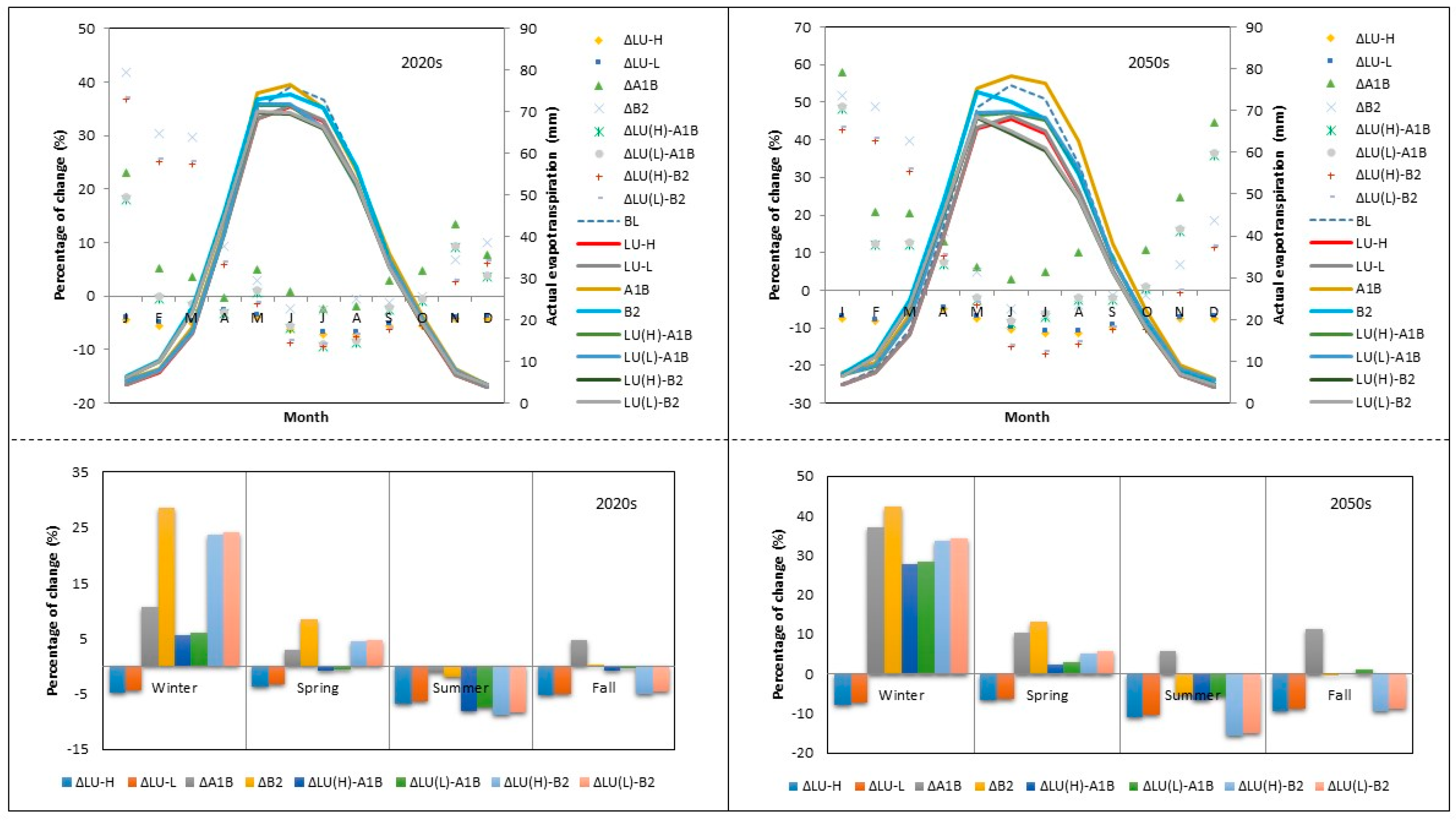
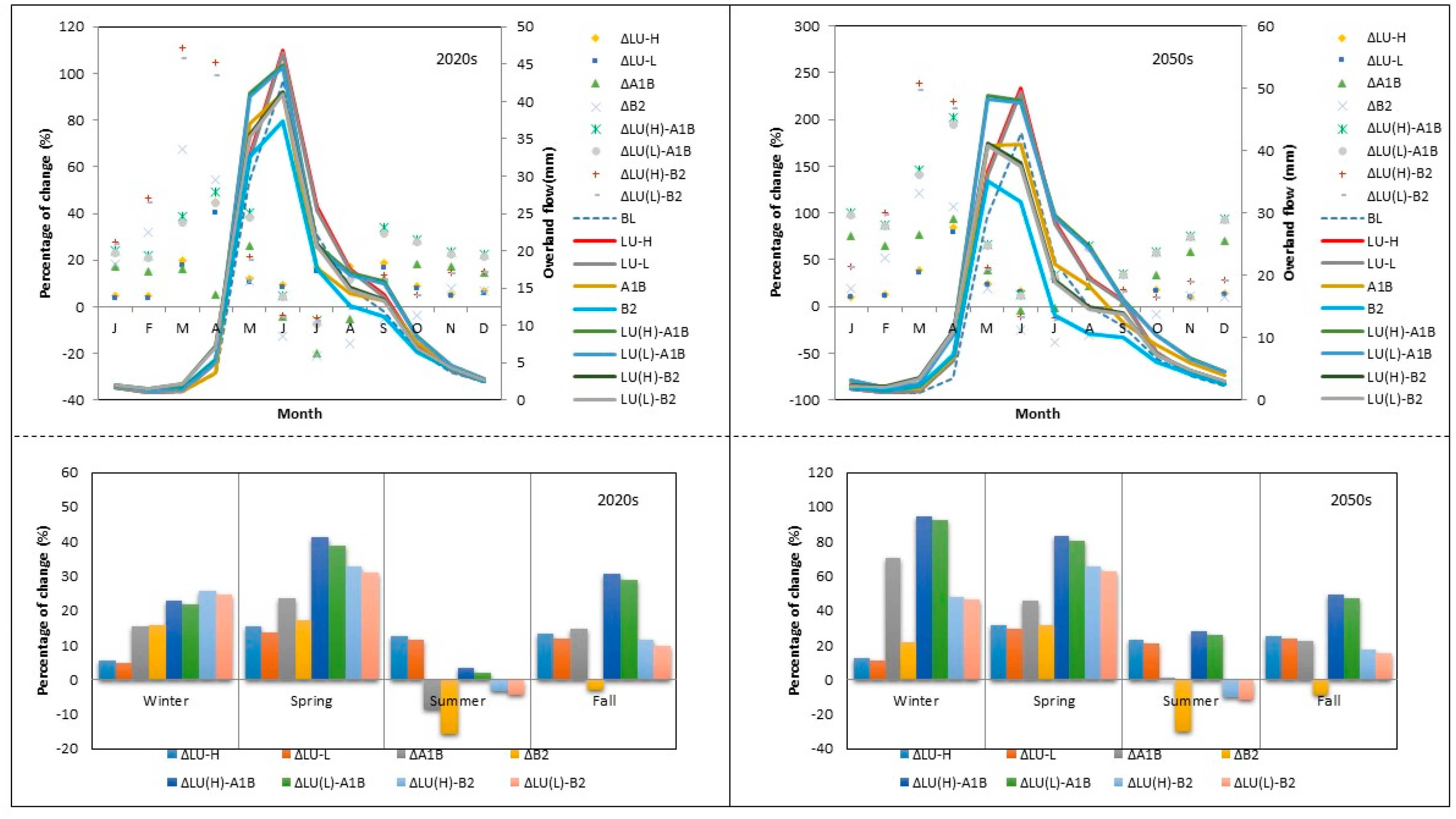
Simulation results (Figure 5) indicate that, in winter, the dominant driver of the ET process is climate change rather than LULC change in both the 2020s and 2050s. During this season, a rise in temperature under the two climate scenarios results in more snowmelt, which in turn creates more water available for evaporation and transpiration from soil and vegetation, respectively. The magnitude of changes is greater under the B2 scenario (28.6–42.2%) compared to the A1B (10.8–36.9%) scenario, due to a larger increase in temperature under the B2 (2.2 °C and 3.2 °C) scenario compared to A1B (0.9 °C and 2.8 °C), in the 2020s and 2050s, respectively. On the other hand, the two LULC change scenarios, LU-H and LU-L, induce not only less modification (−4.8–7.7% and −4.4–7.3%) to ET compared to climate change scenarios in the 2020s and 2050s, but the changes occur in different directions. In spring, the impact of climate change is greater than the influence of LULC change in the 2020s and 2050s, except under the A1B scenario in the 2020s. The largest variation in ET occurs in the summer as a result of two factors: first, a higher atmospheric demand due to higher average air temperature in this season; and, second, an increase in the leaf area, which plays an important role for evapotranspiration especially in the summer when the key control is rainfall interception considering that the highest amount of rainfall occurs during this season. The second factor is mostly attributed to LULC characteristics, meaning that a change in LULC can cause considerable variation in ET in summer compared to other seasons. For instance, a conversion from forest to urban areas results in less canopy and root density, and in turn, more paved areas, which causes a reduction in ET. Figure 5 illustrates that variations in ET in summer due to climate change occur in the same direction as LULC change, which amplifies the combined impact of climate and LULC change. However, this is not the case for the A1B scenario in the 2050, which compensates the impact of LULC change scenarios.
In the fall, the induced changes in ET under the A1B scenario occur in the opposite direction and with almost the same magnitude of changes caused by the LU-H and LU-L scenarios in the 2020s and 2050s. On the other hand, there is a slight change in ET due to the B2 climate scenario indicating that LULC change scenarios are the dominant drivers for the changes in ET in response to combined climate and LULC change scenarios in the 2020s and 2050s. The peak in the watershed ET occurs in June in the baseline period. However, the ET peaks under the B2, LU(H)-B2, and LU(L)-B2 scenarios tend to shift from June to May in the 2050s.

Infiltration

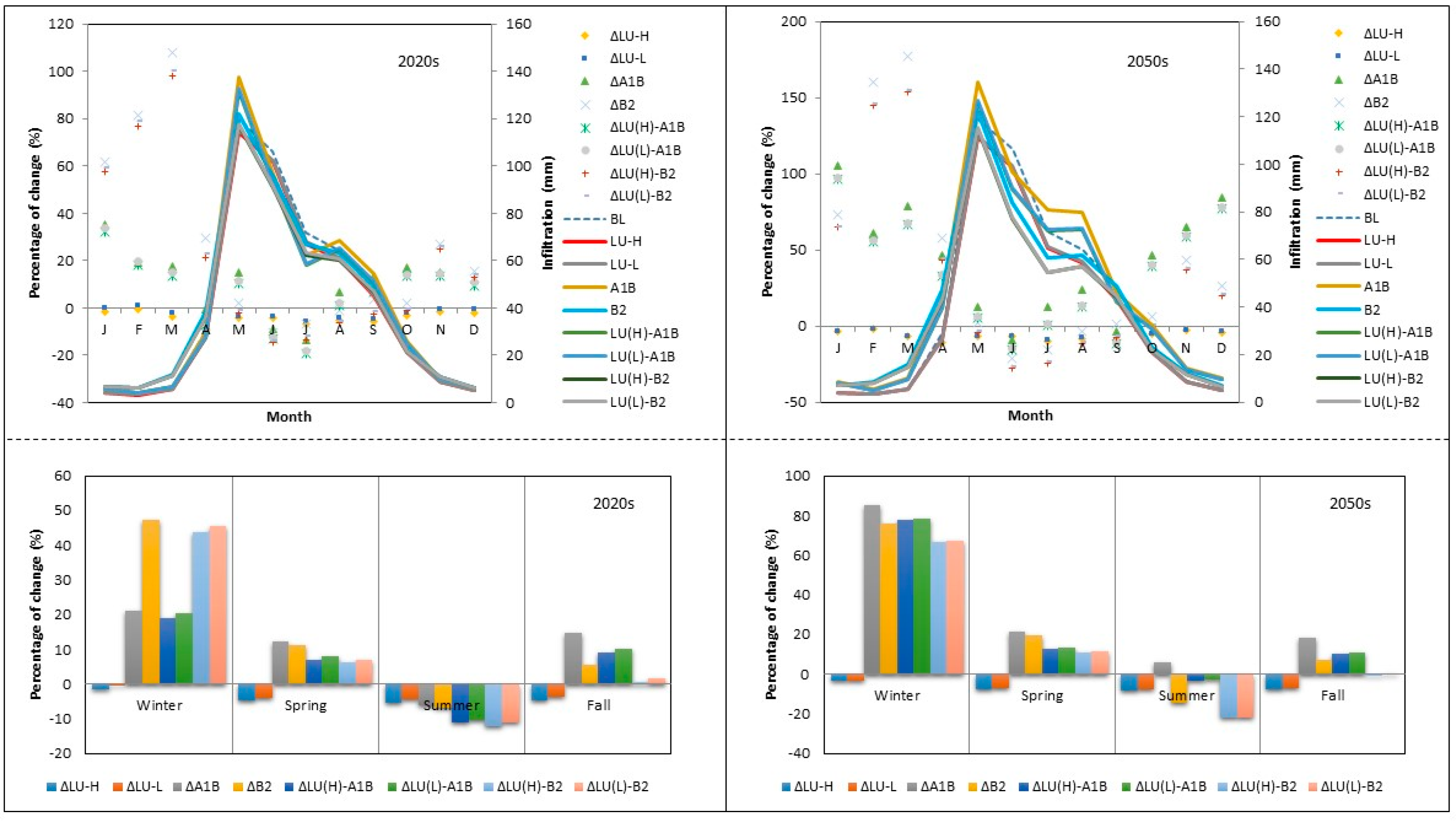
The impact of climate change on infiltration is more pronounced in the winter and spring, whereas the impact of LULC change is more dominant in the summer in the 2020s and 2050s (Figure 6). The greatest change in infiltration occurs in winter under the A1B and B2 scenarios in the 2020s (21.2% and 47.4%) and 2050s (85.3% and 76.1%), respectively. This is mostly attributed to snowmelt due to a rise in temperature. In addition, less saturated soil tends to intensify the infiltration rate in this season. This was also found by Huntington et al. [66] when they investigated the impact of climate change on winter snow regime and infiltration in the northeastern US. The influence of LULC change scenarios on winter infiltration is minimal compared to the impact of climate change.
The response of infiltration to climate change in spring is less pronounced than the response in winter. The soil is more saturated in the spring compared to winter due to higher rates of snow melt. This increases the possibility of reaching the steady-state infiltration rate, which results in a reduction in spring infiltration rates. On the other hand, the influence of LULC change on infiltration increases in the spring, though climate change is still the dominant driver in this season. In the 2020s and 2050s, summer infiltration decreases under both climate and LULC scenarios, except for the A1B scenario in 2050s. The decline under climate change scenarios is associated mostly with a reduction in precipitation, except with the A1B scenario in 2050s that results in an increase in infiltration, likely linked to a rise in precipitation. On the other hand, the decline in infiltration under LULC change scenarios is associated with an increase in impervious surface areas, which is highlighted in the summer when the highest rainfall events occur. This means the more surface areas are impervious, the less infiltration per unit of rainfall occurs in the watershed. In the fall, the impact of LULC change scenarios compensates the influence of the B2 climate scenario in the 2020s and 2050s; however, this is not the case for the A1B scenario.

Overland Flow

In winter, overland flow increases under both, the climate—A1B (15.5% and 70.5%) and B2 (15.7% and 21.8%)—and LULC—LU-H (5.6% and 12.2%) and LU-L (4.8% and 11.2%)—scenarios in the 2020s and 2050s, respectively. The more pronounced impact being driven by climate change (Figure 7). The increase in overland flow is mostly associated with snowmelt due to a rise in temperature. Spring overland flow also increases under all climate—A1B (23.6% and 46.0%) and B2 (17.2% and 31.9%)—and LULC—LU-H (15.6% and 31.7%) and LU-L (13.6% and 29.3%)—scenarios in the 2020s and 2050s, respectively. Snowmelt plays a significant role in spring as well as a result of an increase in temperature in this season. Contributions from climate A1B (−8.6% and 1.4%) and B2 (−15.6% and −30.1%)—and LULC—LU-H (12.8% and 23.0%) and LU-L (11.5% and 21.4%)—scenarios to summer overland flow occur in opposite directions (except with A1B in 2050s), which results in a decline in the magnitude of changes in overland flow under the combined climate and LULC change scenarios. This is mostly due to a decline in precipitation under the A1B scenario in the 2020s, and the B2 scenario in the 2020s and 2050s. On the other hand, a change in LULC due to urbanization can result in more runoff in this season. In fall, overland flow increases under all scenarios A1B (14.7% and 22.3%), LU-H (13.5% and 25.4%), and LU-L (12.1% and 23.7%) in the 2020s and 2050s, respectively, except with the B2 (−2.8% and −8.9%) climate scenario. An increase in air temperature during fall can result in water losses when there is a reduction in the snow storage and evapotranspiration is the dominant factor in the water balance. However, this is not the case for the A1B scenario when there is a considerable rise in precipitation (5.6% and 4.4%) compared to the B2 (1.5% and 0.9%) scenario in the 2020s and 2050s, respectively. The peaks in overland flow occur in June under the LULC scenarios (similar to the baseline scenario) but tend to shift from June to May under the climate and combined climate and LULC scenarios, especially in the 2050s. The largest increase in overland flow occurs in March and April under the LU(H)-B2 scenario in the 2020s and 2050s.

3.2.2. Average Annual Changes in Water Balance

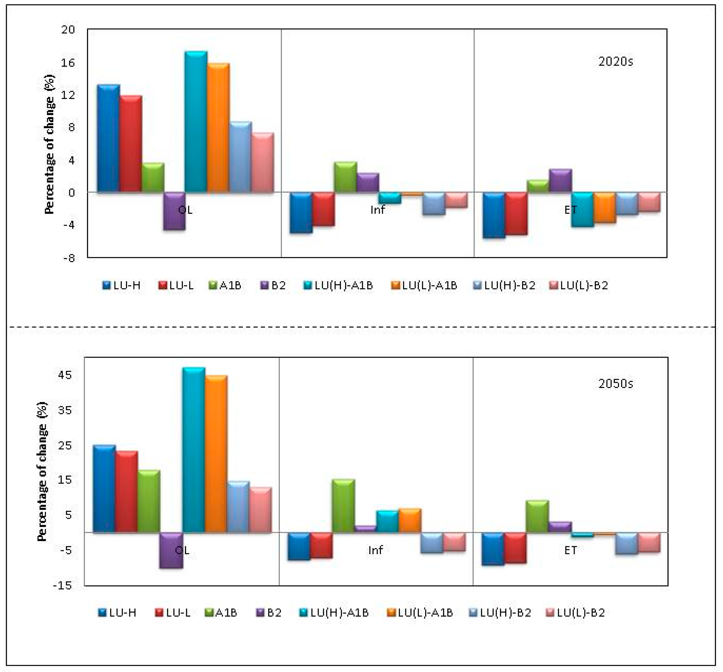
Results reveal that LULC change is the dominant factor effecting the average annual changes in ET (Figure 8). The negative changes (decreases) in ET occur under the LULC change scenarios, LU-H (−5.5% and −9.2%) and LU-L (−5.1% and −8.6%), which compensate the positive changes under the climate scenarios, A1B (1.6 and 9.2%) and B2 (2.9% and 3.1%) in the 2020s and 2050s, respectively. This leads to a negative change in ET under all combined climate and LULC change scenarios, ranging from −2.3% to −4.1% and −0.6% to −6.2% in the 2020s and 2050s, respectively.
LULC change is also the dominant factor affecting infiltration in the 2020s and 2050s, except with the A1B climate scenario in the 2050s. A decrease in the watershed infiltration under LULC change scenarios, LU-H (−4.9% and −7.7%) and LU-L (−4% and −7.2%), compensates the increase observed with the B2 climate scenario (2.4% and 2.1%) in the 2020s and 2050s, respectively. This results in a decline in combined impact of climate and LULC change scenarios, LU(H)-B2 (−2.7% and −5.8%) and LU(L)-B2 (−1.8% and −5.2%), in the 2020s and 2050s, respectively. On the other hand, the impact of LULC change offsets the rise (3.8%) in infiltration under the A1B scenario in the 2020s, resulting in a decline in infiltration under the combined LU(H)-A1B (−1.3%) and LU(L)-A1B (−0.4%) scenarios. However, a rise (15%) in infiltration leads to an increase (6.3% and 6.9%) in infiltration under the LU(H)-A1B and LU(L)-A1B scenarios, in the 2050s, respectively.
The impact of LULC change on overland flow is more pronounced compared to the impact of climate change in the 2020s and 2050s. The responses of overland flow to the LULC change scenarios (LU-H and LU-L) and the A1B climate scenario occur in the same direction. Therefore, the conjunction of the LULC change scenarios with the A1B climate scenario amplifies the magnitude of the rise in overland flow by 17.4% and 15.9% under the LU(H)-A1B and LU(L)-A1B scenarios, respectively. On the other hand, the responses of overland flow to LULC change scenarios (LU-H and LU-L) occur in the opposite direction of changes in overland flow affected by the B2 climate scenario. This leads to a reduction in the magnitude of change in overland flow by 8.7% and 7.3% under the LU(H)-B2 and LU(L)-B2 scenarios, respectively. In the 2050s, changes in overland flow occur with the same directions of the 2020s, but with a higher magnitude but with a higher magnitude, under the LU(H)-B2 (14.6%) and LU(L)-B2 (12.9%) scenarios.

3.2.3. Streamflow

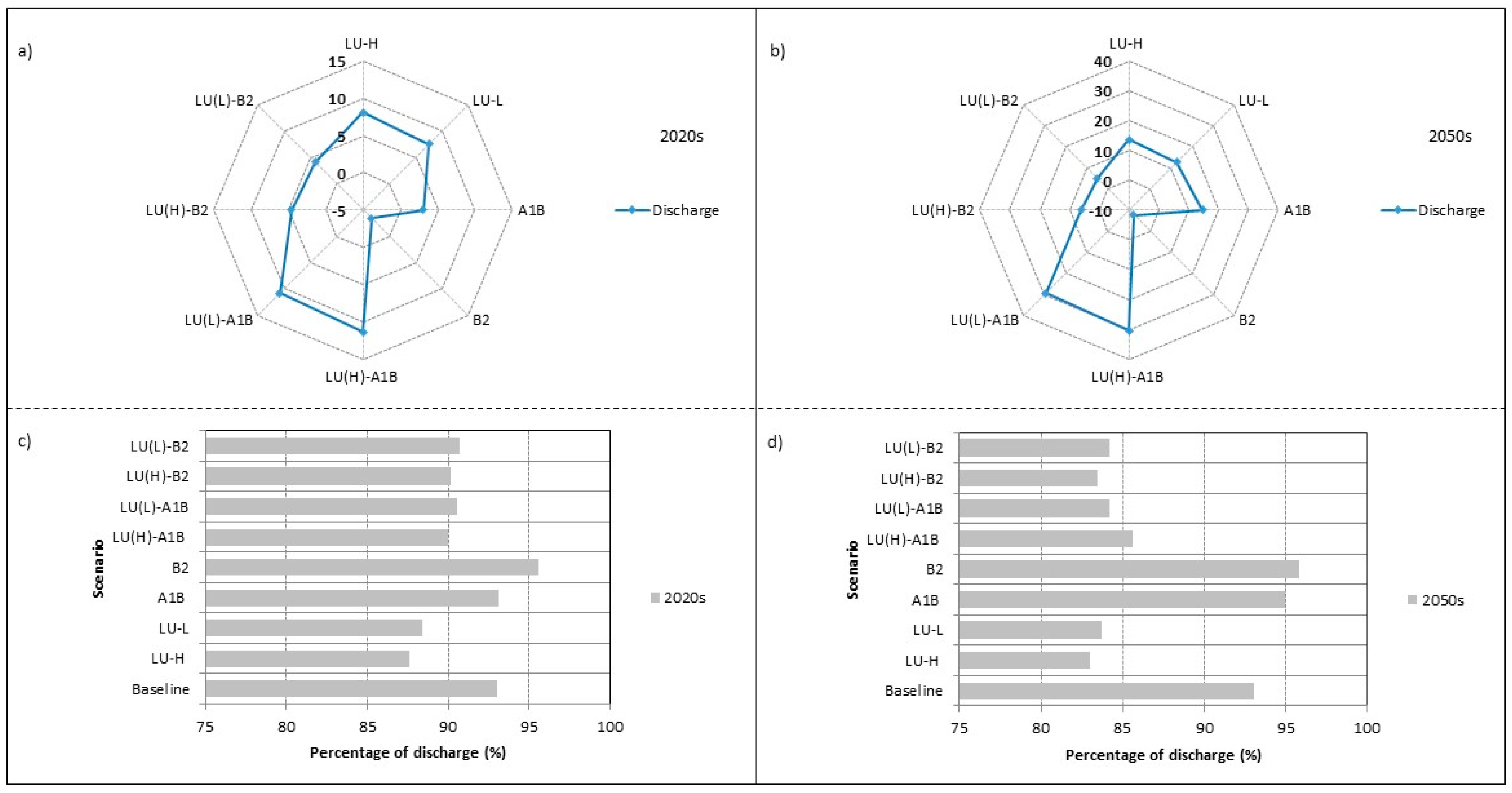
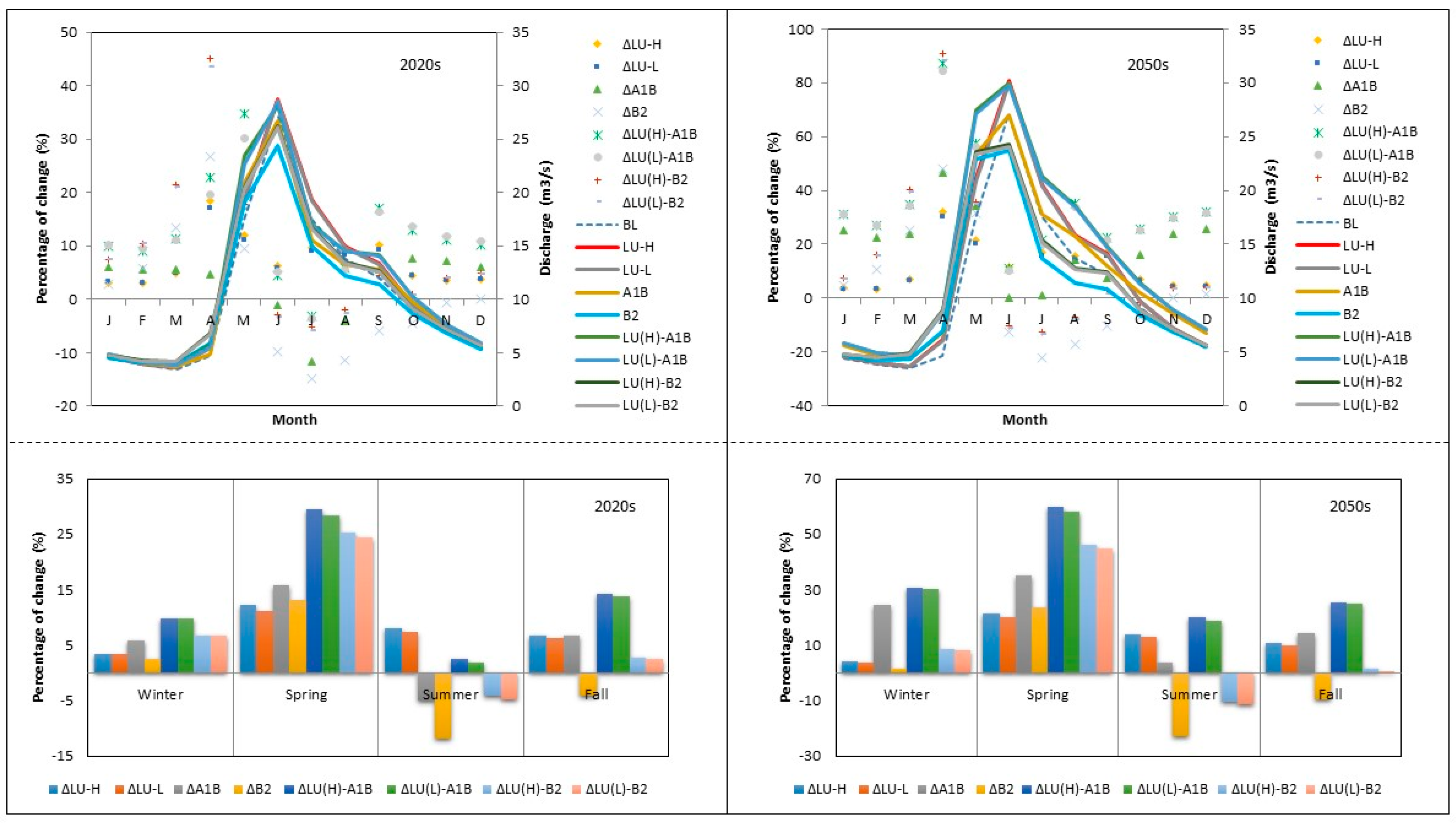
In the 2020s and 2050s, the impact of LULC change on average annual streamflow is more important than the influence of climate change, except with the A1B climate scenario in the 2050s (Figure 9). The LULC change scenarios increase streamflow in the 2020s (8.1% and 7.5%) and 2050s (13.7% and 12.7%). Changes in streamflow under the A1B (3.0% and 14.7%) scenario occur in the same direction as with the LULC scenarios, which result in an increase in streamflow under the LU(H)-A1B (11.4% and 30.5%) and LU(L)-A1B (10.8% and 29.4%) scenarios in the 2020s and 2050s, respectively. On the other hand, LULC scenarios compensate the decline in streamflow under the B2 scenarios in the 2020s and 2050s, respectively.
As mentioned in Section 2.1, a large portion of the average annual discharge (~93%) is generated at the 05BJ004 station, considering 100% of discharge at the 05J010 station (Figure 9). Simulation shows that this proportion of discharge at the 05BJ004 station increases under the climate scenarios while it decreases under the LULC scenarios in the 2020s and 2050s. The former can be associated with different spatial distribution of climate impacts along with different geomorphological characteristics of the watershed, and the latter is due to a change in urbanization of the east sub-catchment that can result in a rise in converted units of rainfall to runoff and snowpack water equivalent. In addition, LULC change compensates the influence of climate change, which results in a decline in the proportion of streamflow generated at the 05BJ004 station due to the combined climate and LULC scenarios in the 2020s and 2050s.
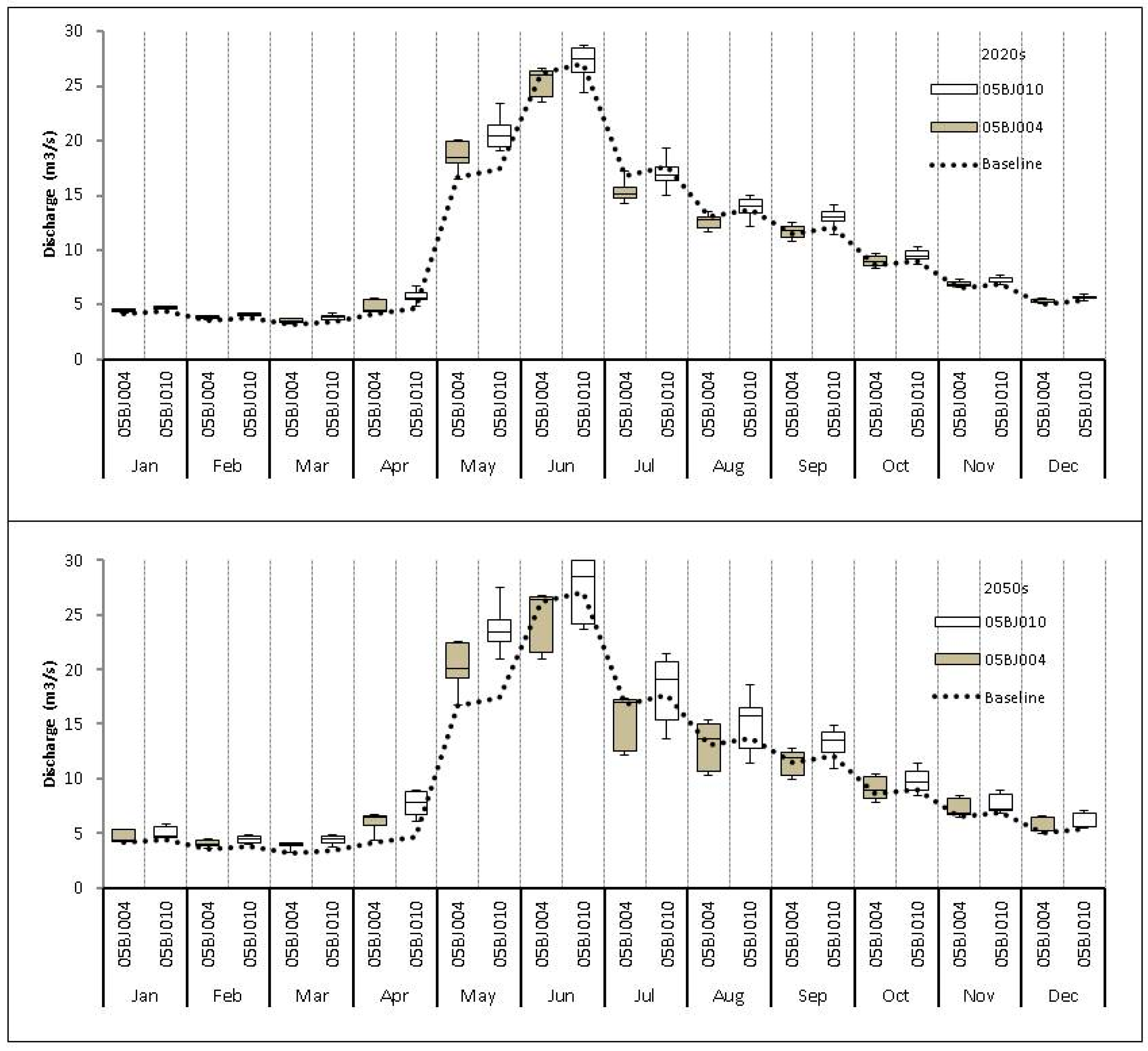
The average seasonal streamflow increases under the combined and individual climate and LULC change scenarios in the winter and spring of the 2020s and 2050s (Figure 10 and Figure 11). During these seasons, streamflow is strongly attributed to snowmelt, which in turn is more controlled by variations in temperature than precipitation. At high elevations in the watershed, precipitation falls predominantly as snow in the winter and accumulates in storage until spring melt, although snowmelt occurs in winter especially at low elevations when temperatures are above freezing, which results in a low flow through winter and early spring. In 2020s, winter streamflow increases under the A1B and B2 climate change scenarios by 5.9% and 2.5%, respectively, while it also increases under the LULC change scenarios by 3.4%. The direction of the change in streamflow affected by LULC change-alone and climate change-alone is the same; therefore, the rise in streamflow is enhanced in response to the combined climate and LULC scenarios. In the 2050s, the magnitude of change in winter streamflow under the A1B scenario (24.6%) is considerably larger than under the B2 scenario (1.6%); this can be associated with a rise in precipitation. This results in greater streamflow under the combined climate and LULC change scenarios, LU(H)-A1B and LU(L)-A1B, compared to the LU(H)-B2 and LU(L)-B2 scenarios. On the other hand, streamflow increases by 3.8–4% under the LULC scenarios, which is not a considerable change compared to A1B (24.6%); however it is greater than the increase under the B2 scenario (1.6%).
In spring, streamflow exhibits the largest variations in both the 2020s and 2050s. The greatest changes in spring occur under the LU(H)-A1B and LU(L)-A1B scenarios in the 2020s (28.3–29.4%) and 2050s (58.2–59.8%), respectively. This is mostly associated with the A1B climate scenario, which is the dominant driver compared to the LULC change scenarios and the B2 climate scenario. Streamflow increases considerably in the late spring for both climate scenarios due to a considerable rise in precipitation along with an increase in snowmelt. High flows can be even further amplified especially in the late spring when an increase in temperature can lead to a rise in a number of rain-on-snow events and eventually enhance the risk of flooding. Although there is a decline in precipitation under the B2 scenario in the 2020s, streamflow exhibits an increase in this season, which implies an intensified snowmelt.
In the summer, the climate change scenarios generate a decline in streamflow in the 2020s and 2050s, except with the A1B scenario in the 2050s when a slight increase can be observed. On the other hand, LULC change results in an increase in summer streamflow. Increasing streamflow in many watersheds has been attributed to LULC change [67,68,69,70]. A change in LULC due to urbanization and deforestation can result in a decline in rainfall interception loss, canopy evapotranspiration, and a rise in converted units of rainfall to runoff and snowpack water equivalent. These changes are more pronounced in the summer when streamflow tends to respond directly and quickly to the precipitation that falls on the ground, mainly as rain. Simulation of summer streamflow indicates a rise under the LULC change scenarios, LU-H (8.1%) and LU-L (7.4%), in the 2020s. A rise in streamflow under the LU-H (8.1%) and LU-L (7.4%) scenarios creates a buffering effect on declining streamflow under the A1B (−5%) climate scenario, and eventually results in an increased streamflow under the LU(H)-A1B (2.4%) and LU(L)-A1B (1.8%) scenarios. However, the rise in streamflow affected by the LULC change scenarios cannot offset the decline in streamflow affected by the B2 (−11.8%) climate scenario, which results in a decrease in streamflow under the combined LU(L)-B2 (−4.1%) and LU(H)-B3(3) (−4.7%), scenarios. In the 2050s, the direction of changes in streamflow in the summer is the same as the 2020s, but with a higher magnitude, except for the A1B climate scenario, which causes a rise (3.7%) in streamflow in the 2050s and enhances the increase in LU(H)-A1B (19.9%) and LU(L)-A1B (18.8%).
In the fall, an increase in temperature can result in more water losses by evapotranspiration from the watershed, rather than a rise in the snowmelt when snowpack reaches a lower volume. Simulation shows that an increase in streamflow due to the LULC change scenarios and the A1B climate change scenario amplifies the rise in streamflow under the combined LU(H)-A1B (14.3–25.4%) and LU(L)-A1B (13.9–24.7%) scenarios in the 2020s and 2050s, respectively. However, the B2 scenario compensates the LULC change impact and results in a small rise in streamflow in the LU(H)-B2 and LU(L)-B2 scenarios.

Flow Duration Curve

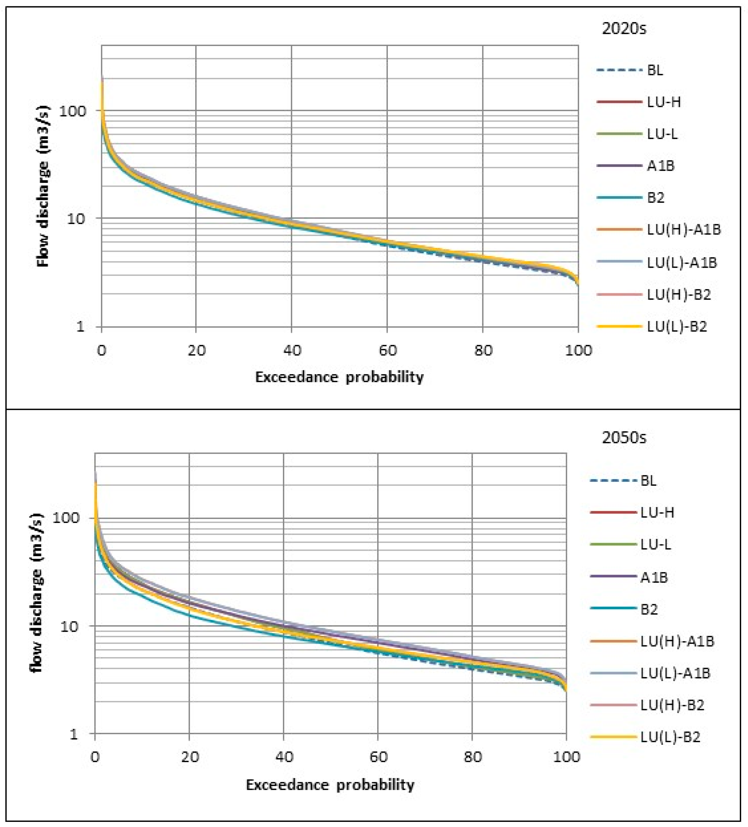
Flow duration curves (FDCs) were generated for each scenario and the baseline in the 2020s and 2050s (Figure 12). They were evaluated at the Q5 (representing peak flows), Q50 (representing mid-range average flow inflection point), and Q90 (representing low flows) discharges, related to baseline in the 2020s and 2050s. Discharge values at Q5 reveal that the LULC contribution to peak flows is more important than the contribution of climate change in the watershed for both 2020s and 2050s, which is not the case for the average (Q50) and low (Q95) discharge flows. High flows in the watershed occur in the summer, and a change in LULC due to urbanization and deforestation can cause a rise in converted units of rainfall to runoff. In other words, LULC change may have more effects on floods rather than droughts and normal discharge flows in the watershed. The influence of LULC change on the peak flow magnitude can be intensified when it occurs in the same direction as climate change impacts.

4. Conclusions

The hydrological processes in the Elbow River watershed exhibit a complex behaviour due to multiple factors such as the seasonal and spatial patterns of snow and rainfall, temperature, climatic gradients associated with altitude, heterogeneity of the land surface, and geomorphology. This complexity can be further enhanced due to projected changes in climate and LULC.
This paper describes the hydrological responses of the watershed under two extreme climate and LULC scenarios over the next 60 years using an integrated modeling system that incorporates the major components of climate, LULC, and hydrology. Results indicate that both LULC and climate change introduce considerable modifications to the hydrological processes, annually and seasonally. Simulations reveal that the LULC change scenarios increase the average annual streamflow, which amplifies the magnitude of rise associated with the A1B climate scenario and compensates for the decline linked to the B2 climate scenario.
Seasonal patterns reveal that the largest rise in streamflow occurs in spring under both the climate and LULC scenarios. Streamflow is strongly attributed to snowmelt in this season which is more controlled by variations in temperature than precipitation. High flows can be even further amplified especially in the late spring when an increase in temperature can lead to a rise in a number of rain-on-snow events and eventually enhance the risk of flooding. The flow duration curves indicate that LULC change causes an increase in peak flows in both the 2020s and 2050s. A change in LULC due to urbanization and deforestation can result in a decline in rainfall interception loss, canopy evapotranspiration, and a rise in converted units of rainfall to runoff and snowpack water equivalent. These changes are more pronounced in the summer when streamflow tends to respond directly and quickly to the precipitation that falls on the ground, mainly as rain. The separated impacts of climate and LULC change on streamflow are positively correlated in winter and spring, which intensifies their combined influence and may also increase the vulnerability of the watershed to floods in spring. LULC change results in a decline in actual evapotranspiration and infiltration and a rise in overland flow and streamflow in all seasons.
The proposed integrated modelling system not only captured the complex interactions between climate, land, and hydrology, but also highlighted the nonlinear mechanism and underlying processes of the system components. For example, even a small magnitude of change in a climate variable may influence hydrological components differently depending on the season. For example, a rise in temperature during winter, spring, and early summer may result in a rise in runoff when snow is the dominant factor in the watershed. On the other hand, an increase in air temperature during fall and late summer may result in water losses when there is a reduction in the snow storage and evapotranspiration is the dominant factor in the water balance. This can be more complex when precipitation and temperature tend to offset each other’s influence differently in different seasons.
The findings of this study highlighted the fact that LULC and climate changes can amplify or offset each other’s impact on hydrological processes based on the direction and magnitude of their influence. Investigating the hydrological responses to climate change-alone or LULC change-alone may lead to an underestimation or overestimation of the hydrological response of a watershed. This study strongly suggests that water resources management and adaptation policies should incorporate the impact of both climate and LULC factors on hydrological responses, particularly in urban watersheds.

Acknowledgments

This project was funded by Tecterra, Alberta Environment and Parks (AEP), and Alberta Innovates Technology Futures. We thank Patrick Delaney and Ying Qiao from DHI Water and Environment Canada, and Mohammad Reza Najafi from Pacific Climate Impacts Consortium, University of Victoria for their insightful support.

Author Contributions

Babak Farjad conducted data collection, wrote the paper, designed and implemented the method, performed simulation and data analysis, and interpreted results. Anil Gupta and Danielle J. Marceau supervised the project, participated in helping in all steps of the project from the beginning until the end. Saman Razavi and Monireh Faramarzi participated in reviewing of the manuscript, evaluation of the method, results and interpretation.

Conflicts of Interest

The authors declare no conflict of interest.

Appendix A

Figure A1. Location of the climate stations in the watershed.
Water 09 00767 g013

Appendix B

Table A1. Elevation of the climate stations in the watershed.
Climate Station (ID)Elevation
30310901067
30318751235
303FOPP1303
30522701400
30536021463
305LRKB2120

References

  1. Legesse, D.; Vallet-Coulomb, C.; Gasse, F. Hydrological response of a catchment to climate and land use changes in Tropical Africa: Case study South Central Ethiopia. J. Hydrol. 2003, 275, 67–85. [Google Scholar] [CrossRef]
  2. Li, Z.; Liu, W.Z.; Zhang, X.C.; Zheng, F.L. Impacts of land use change and climate variability on hydrology in an agricultural catchment on the Loess Plateau of China. J. Hydrol. 2009, 377, 35–42. [Google Scholar] [CrossRef]
  3. Gathenya, M.; Mwangi, H.; Coe, R.; Sang, J. Climate-and land use-induced risks to watershed services in the Nyando River Basin, Kenya. Exp. Agric. 2011, 47, 339–356. [Google Scholar] [CrossRef]
  4. Weatherhead, E.K.; Howden, N.J.K. The relationship between land use and surface water resources in the UK. Land Use Policy 2009, 26, S243–S250. [Google Scholar] [CrossRef]
  5. Dias, L.C.P.; Macedo, M.N.; Costa, M.H.; Coe, M.T.; Neill, C. Effects of land cover change on evapotranspiration and streamflow of small catchments in the Upper Xingu River Basin, Central Brazil. J. Hydrol. Reg. Stud. 2015, 4, 108–122. [Google Scholar] [CrossRef]
  6. Hundecha, Y.; Bárdossy, A. Modeling of the effect of land use changes on the runoff generation of a river basin through parameter regionalization of a watershed model. J. Hydrol. 2004, 292, 281–295. [Google Scholar] [CrossRef]
  7. Kundzewicz, Z.W.; Mata, L.J.; Arnell, N.W.; Döll, P.; Jimenez, B.; Miller, K.; Oki, T.; Şen, Z.; Shiklomanov, I. The implications of projected climate change for freshwater resources and their management. Hydrol. Sci. J. 2008, 53, 3–10. [Google Scholar] [CrossRef]
  8. Farjad, B.; Gupta, A.; Marceau, D.J. Hydrological regime responses to climate change for the 2020s and 2050s periods in the Elbow River watershed in southern Alberta, Canada. In Environmental Management of River Basin Ecosystems; Springer: Cham, Switzerland, 2015; pp. 65–89. [Google Scholar]
  9. Farjad, B.; Gupta, A.; Marceau, D.J. Annual and Seasonal Variations of Hydrological Processes under Climate Change Scenarios in Two Sub-Catchments of a Complex Watershed. Water Resour. Manag. 2016, 30, 2851–2865. [Google Scholar] [CrossRef]
  10. Bell, R.; Hodges, K.; Vidale, P.L.; Strachan, J.; Roberts, M. Simulation of the global ENSO–tropical cyclone teleconnection by a high-resolution coupled general circulation model. J. Clim. 2014, 27, 6404–6422. [Google Scholar] [CrossRef]
  11. Lehner, B.; Döll, P.; Alcamo, J.; Henrichs, T.; Kaspar, F. Estimating the impact of global change on flood and drought risks in Europe: A continental, integrated analysis. Clim. Chang. 2006, 75, 273–299. [Google Scholar] [CrossRef]
  12. Hosseinizadeh, A.; SeyedKaboli, H.; Zareie, H.; Ali, M.A.; Farjad, B. Impact of climate change on the severity, duration and frequency of drought in a semi-arid agricultural basin. Geoenviron. Disasters 2015, 2, 1–9. [Google Scholar] [CrossRef]
  13. Loukas, A.; Quick, M.C. The Effect of Climate Change on Hydrologic Regime of Two Climatically Different Watersheds. ASCE J. Hydrol. Eng. 1996, 1, 77–87. [Google Scholar] [CrossRef]
  14. Boyer, C.; Chaumont, D.; Chartier, I.; Roy, A.G. Impact of climate change on the hydrology of St. Lawrence tributaries. J. Hydrol. 2010, 384, 65–83. [Google Scholar] [CrossRef]
  15. Barron, O.; Silberstein, R.; Ali, R.; Donohue, R.; McFarlane, D.J.; Davies, P.; Donn, M. Climate change effects on water-dependent ecosystems in south-western Australia. J. Hydrol. 2012, 434, 95–109. [Google Scholar] [CrossRef]
  16. Dibike, Y.B.; Coulibaly, P. Hydrologic impact of climate change in the Saguenay watershed: Comparison of downscaling methods and hydrologic models. J. Hydrol. 2005, 307, 145–163. [Google Scholar] [CrossRef]
  17. Forbes, K.A.; Kienzle, S.W.; Coburn, C.A.; Byrne, J.M.; Rasmussen, J. Simulating the hydrological response to predicted climate change on a watershed in southern Alberta, Canada. Clim. Chang. 2011, 105, 555–576. [Google Scholar] [CrossRef]
  18. He, J.; Valeo, C.; Chu, A.; Neumann, N.F. Stormwater quantity and quality response to climate change using artificial neural networks. Hydrol. Process 2011, 25, 1298–1312. [Google Scholar] [CrossRef]
  19. Chen, J.; Brissette, F.P.; Poulin, A.; Leconte, R. Overall uncertainty study of the hydrological impacts of climate change for a Canadian watershed. Water Resour. Res. 2011, 47. [Google Scholar] [CrossRef]
  20. Kienzle, S.W.; Nemeth, M.W.; Byrne, J.M.; MacDonald, R.J. Simulating the hydrological impacts of climate change in the upper North Saskatchewan River basin, Alberta, Canada. J. Hydrol. 2012, 412, 76–89. [Google Scholar] [CrossRef]
  21. Gädeke, A.; Hölzel, H.; Koch, H.; Pohle, I.; Grünewald, U. Analysis of uncertainties in the hydrological response of a model-based climate change impact assessment in a subcatchment of the Spree River, Germany. Hydrol. Process. 2014, 28, 3978–3998. [Google Scholar] [CrossRef]
  22. Velázquez, J.A.; Schmid, J.; Ricard, S.; Muerth, M.J.; St-Denis, B.G.; Minville, M.; Turcotte, R. An ensemble approach to assess hydrological models’ contribution to uncertainties in the analysis of climate change impact on water resources. Hydrol. Earth Syst. Sci. 2013, 17, 565. [Google Scholar] [CrossRef]
  23. Poulin, A.; Brissette, F.; Leconte, R.; Arsenault, R.; Malo, J.S. Uncertainty of hydrological modelling in climate change impact studies in a Canadian, snow-dominated river basin. J. Hydrol. 2011, 409, 626–636. [Google Scholar] [CrossRef]
  24. Najafi, M.R.; Moradkhani, H.; Jung, I.W. Assessing the uncertainties of hydrologic model selection in climate change impact studies. Hydrol. Process. 2011, 25, 2814–2826. [Google Scholar] [CrossRef]
  25. Nolan, P.; O’Sullivan, J.; McGrath, R. Impacts of climate change on mid-twenty-first-century rainfall in Ireland: A high-resolution regional climate model ensemble approach. Int. J. Climatol. 2017. [Google Scholar] [CrossRef]
  26. Chaudhuri, C.; Srivastava, R. A novel approach for statistical downscaling of future precipitation over the Indo-Gangetic Basin. J. Hydrol. 2017, 547, 21–38. [Google Scholar] [CrossRef]
  27. Bronstert, A. Rainfall-runoff modelling for assessing impacts of climate and land-use change. Hydrol. Process. 2004, 18, 567–570. [Google Scholar] [CrossRef]
  28. Thanapakpawin, P.; Richey, J.; Thomas, D.; Rodda, S.; Campbell, B.; Logsdon, M. Effects of landuse change on the hydrologic regime of the Mae Chaem river basin, NW Thailand. J. Hydrol. 2007, 334, 215–230. [Google Scholar] [CrossRef]
  29. Wijesekara, G.N.; Farjad, B.; Gupta, A.; Qiao, Y.; Delaney, P.; Marceau, D.J. A Comprehensive Land-Use/Hydrological Modeling System for Scenario Simulations in the Elbow River Watershed, Alberta, Canada. Environ. Manag. 2014, 53, 357–381. [Google Scholar] [CrossRef] [PubMed]
  30. Jakeman, A.J.; Littlewood, I.G.; Whitehead, P.G. An assessment of the dynamic response characteristics of streamflow in the Balquhidder catchments. J. Hydrol. 1993, 145, 337–355. [Google Scholar] [CrossRef]
  31. Abbott, M.B.; Bathurst, J.C.; Cunge, J.A.; O’Connell, P.E.; Rasmussen, J. An introduction to the European Hydrological System—Système Hydrologique Européen, “SHE”, 1: History and philosophy of a physically-based, distributed modelling system. J. Hydrol. 1986, 87, 45–59. [Google Scholar] [CrossRef]
  32. Dunn, S.M.; Mackay, R. Spatial variation in evapotranspiration and the influence of land use on catchment hydrology. J. Hydrol. 1995, 171, 49–73. [Google Scholar] [CrossRef]
  33. Hendriks, M. Introduction to Physical Hydrology; Oxford University Press: Oxford, UK, 2010; p. 331. [Google Scholar]
  34. Notebaert, B.; Verstraeten, G.; Ward, P.; Renssen, H.; Van Rompaey, A. Modeling the sensitivity of sediment and water runoff dynamics to Holocene climate and land use changes at the catchment scale. Geomorphology 2011, 126, 18–31. [Google Scholar] [CrossRef]
  35. Tu, J. Combined impact of climate and land use changes on streamflow and water quality in eastern Massachusetts, USA. J. Hydrol. 2009, 379, 268–283. [Google Scholar] [CrossRef]
  36. Antonellini, M.; Dentinho, T.; Khattabi, A.; Masson, E.; Mollema, P.N.; Silva, V.; Silveira, P. An integrated methodology to assess future water resources under land use and climate change: An application to the Tahadart drainage basin (Morocco). Environ. Earth Sci. 2014, 71, 1839–1853. [Google Scholar] [CrossRef]
  37. Gan, T.Y.; Burges, S.J. An assessment of a conceptual rainfall-runoff model’s ability to represent the dynamics of small hypothetical catchments: 2. Hydrologic responses for normal and extreme rainfall. Water Resour. Res. 1990, 26, 1605–1619. [Google Scholar]
  38. Khoi, D.N.; Suetsugi, T. The responses of hydrological processes and sediment yield to land-use and climate change in the Be River Catchment, Vietnam. Hydrol. Process. 2014, 28, 640–652. [Google Scholar] [CrossRef]
  39. Montenegro, S.; Ragab, R. Impact of possible climate and land use changes in the semi arid regions: A case study from North Eastern Brazil. J. Hydrol. 2012, 434, 55–68. [Google Scholar] [CrossRef]
  40. Wilbanks, T.J.; Kates, R.W. Global change in local places: How scale matters. Clim. Chang. 1999, 43, 601–628. [Google Scholar] [CrossRef]
  41. Strengers, B.; Leemans, R.; Eickhout, B.; de Vries, B.; Bouwman, L. The land-use projections and resulting emissions in the IPCC SRES scenarios as simulated by the IMAGE 2.2 model. GeoJournal 2004, 61, 381–393. [Google Scholar] [CrossRef]
  42. Sleeter, B.M.; Sohl, T.L.; Bouchard, M.A.; Reker, R.R.; Soulard, C.E.; Acevedo, W.; Zhu, Z. Scenarios of land use and land cover change in the conterminous United States: Utilizing the special report on emission scenarios at ecoregional scales. Glob. Environ. Chang. 2012, 22, 896–914. [Google Scholar] [CrossRef]
  43. Kankaanpää, S.; Carter, T.R. Construction of European Forest Land Use Scenarios for the 21st Century; Finnish Environment Institute: Helsinki, Finland, 2004; p. 57. [Google Scholar]
  44. Verburg, P.H.; Schulp, C.J.E.; Witte, N.; Veldkamp, A. Downscaling of land use change scenarios to assess the dynamics of European landscapes. Agric. Ecosyst. Environ. 2006, 114, 39–56. [Google Scholar] [CrossRef]
  45. Abildtrup, J.; Audsley, E.; Fekete-Farkas, M.; Giupponi, C.; Gylling, M.; Rosato, P.; Rounsevell, M. Socio-economic scenario development for the assessment of climate change impacts on agricultural land use: A pairwise comparison approach. Environ. Sci. Policy 2006, 9, 101–115. [Google Scholar] [CrossRef]
  46. Rounsevell, M.D.A.; Reginster, I.; Araújo, M.B.; Carter, T.R.; Dendoncker, N.; Ewert, F.; Tuck, G. A coherent set of future land use change scenarios for Europe. Agric. Ecosyst. Environ. 2006, 114, 57–68. [Google Scholar] [CrossRef]
  47. Solecki, W.D.; Oliveri, C. Downscaling climate change scenarios in an urban land use change model. J. Environ. Manag. 2004, 72, 105–115. [Google Scholar] [CrossRef] [PubMed]
  48. Tong, S.T.; Sun, Y.; Ranatunga, T.; He, J.; Yang, Y.J. Predicting plausible impacts of sets of climate and land use change scenarios on water resources. Appl. Geogr. 2012, 32, 477–489. [Google Scholar] [CrossRef]
  49. Wang, R.; Kalin, L.; Kuang, W.; Tian, H. Individual and combined effects of land use/cover and climate change on Wolf Bay watershed streamflow in southern Alabama. Hydrol. Process. 2014, 28, 5530–5546. [Google Scholar] [CrossRef]
  50. Alberta Treasury Board and Finance, Alberta Population Projections, by Census Division. 2014. Available online: http://finance.alberta.ca/aboutalberta/population-projections/index.html (accessed on 31 July 2015).
  51. Gan, T.Y. Hydroclimatic trends and possible climatic warming in the Canadian Prairies. Water Resour. Res. 1998, 34, 3009–3015. [Google Scholar] [CrossRef]
  52. He, M.; Hogue, T.S. Integrating hydrologic modeling and land use projections for evaluation of hydrologic response and regional water supply impacts in semi-arid environments. Environ. Earth Sci. 2012, 65, 1671–1685. [Google Scholar] [CrossRef]
  53. GeoBase. 2008. Available online: www.Geobase.ca (accessed on 9 October 2017).
  54. Di Baldassarre, G.; Montanari, A. Uncertainty in river discharge observations: A quantitative analysis. Hydrol. Earth Syst. Sci. 2009, 13, 913. [Google Scholar] [CrossRef]
  55. Zhang, S.; Gao, X.; Zhang, X.; Hagemann, S. Projection of glacier runoff in Yarkant River basin and Beida River basin, Western China. Hydrol. Process 2012, 26, 2773–2781. [Google Scholar] [CrossRef]
  56. Zhang, X.C.; Liu, W.Z.; Li, Z.; Chen, J. Trend and uncertainty analysis of simulated climate change impacts with multiple GCMs and emission scenarios. Agric. For. Meteorol. 2011, 151, 1297–1304. [Google Scholar] [CrossRef]
  57. Snover, A.K.; Hamlet, A.F.; Lettenmaier, D.P. Climate-change scenarios for water planning studies: Pilot applications in the Pacific Northwest. Bull. Am. Meteorol. Soc. 2003, 84, 1513–1518. [Google Scholar] [CrossRef]
  58. Hay, L.E.; McCabe, G.J. Hydrologic effects of climate change in the Yukon River Basin. Clim. Chang. 2010, 100, 509–523. [Google Scholar] [CrossRef]
  59. Arnell, N.W.; Reynard, N.S. The effects of climate change due to global warming on river flows in Great Britain. J. Hydrol. 1996, 183, 397–424. [Google Scholar] [CrossRef]
  60. Köplin, N.; Schädler, B.; Viviroli, D.; Weingartner, R. The importance of glacier and forest change in hydrological climate-impact studies. Hydrol. Earth Syst. Sci. 2013, 17, 619–635. [Google Scholar] [CrossRef] [Green Version]
  61. Hargreaves, G.H.; Samani, Z.A. Reference Crop Evapotranspiration from Ambient Air Temperature; American Society of Agricultural Engineers: St. Joseph, MI, USA, 1985; p. 85. [Google Scholar]
  62. Sentelhas, P.C.; Gillespie, T.J.; Santos, E.A. Evaluation of FAO Penman–Monteith and alternative methods for estimating reference evapotranspiration with missing data in Southern Ontario, Canada. Agric. Water Manag. 2010, 97, 635–644. [Google Scholar] [CrossRef]
  63. Espadafor, M.; Lorite, I.J.; Gavilán, P.; Berengena, J. An analysis of the tendency of reference evapotranspiration estimates and other climate variables during the last 45 years in Southern Spain. Agric. Water Manag. 2011, 98, 1045–1061. [Google Scholar] [CrossRef]
  64. Kristensen, K.J.; Jensen, S.E. A model for estimating actual evapotranspiration from potential evapotranspiration. Nordic Hydrol. 1975, 6, 170–188. [Google Scholar]
  65. Yan, J.; Smith, K.R. Simulation of integrated surface water and ground water system-model formulation. J. Am. Water Resour. Assoc. 1994, 30, 879–890. [Google Scholar] [CrossRef]
  66. Huntington, T.G.; Sheffield, J.; Hayhoe, K. Impacts of climate change on wintertime precipitation, snowmelt regime, surface runoff, and infiltration in the northeastern USA during the 21st century. In Proceedings of the 64th Eastern Snow Conference, St. Johns, NL, Canada, 29 May–1 June 2007; Volume 29, pp. 181–189. [Google Scholar]
  67. Troendle, C.A.; Olsen, W.K. Potential effects of timber harvest and water management on streamflow dynamics and sediment transport. In Sustainable Ecological Systems: Implementing an Ecological Approach to Land Management. USDA Forest Service General Technical Report RM-247; U.S. Department of Agriculture: Fort Collins, CO, USA, 1994; pp. 34–41. [Google Scholar]
  68. Costa, M.H.; Botta, A.; Cardille, J.A. Effects of large-scale changes in land cover on the discharge of the Tocantins River, Southeastern Amazonia. J. Hydrol. 2003, 283, 206–217. [Google Scholar] [CrossRef]
  69. Zhang, Y.K.; Schilling, K.E. Increasing streamflow and baseflow in Mississippi River since the 1940s: Effect of land use change. J. Hydrol. 2006, 324, 412–422. [Google Scholar] [CrossRef]
  70. Peña-Arancibia, J.L.; van Dijk, A.I.; Guerschman, J.P.; Mulligan, M.; Bruijnzeel, L.A.; McVicar, T.R. Detecting changes in streamflow after partial woodland clearing in two large catchments in the seasonal tropics. J. Hydrol. 2012, 416, 60–71. [Google Scholar] [CrossRef]
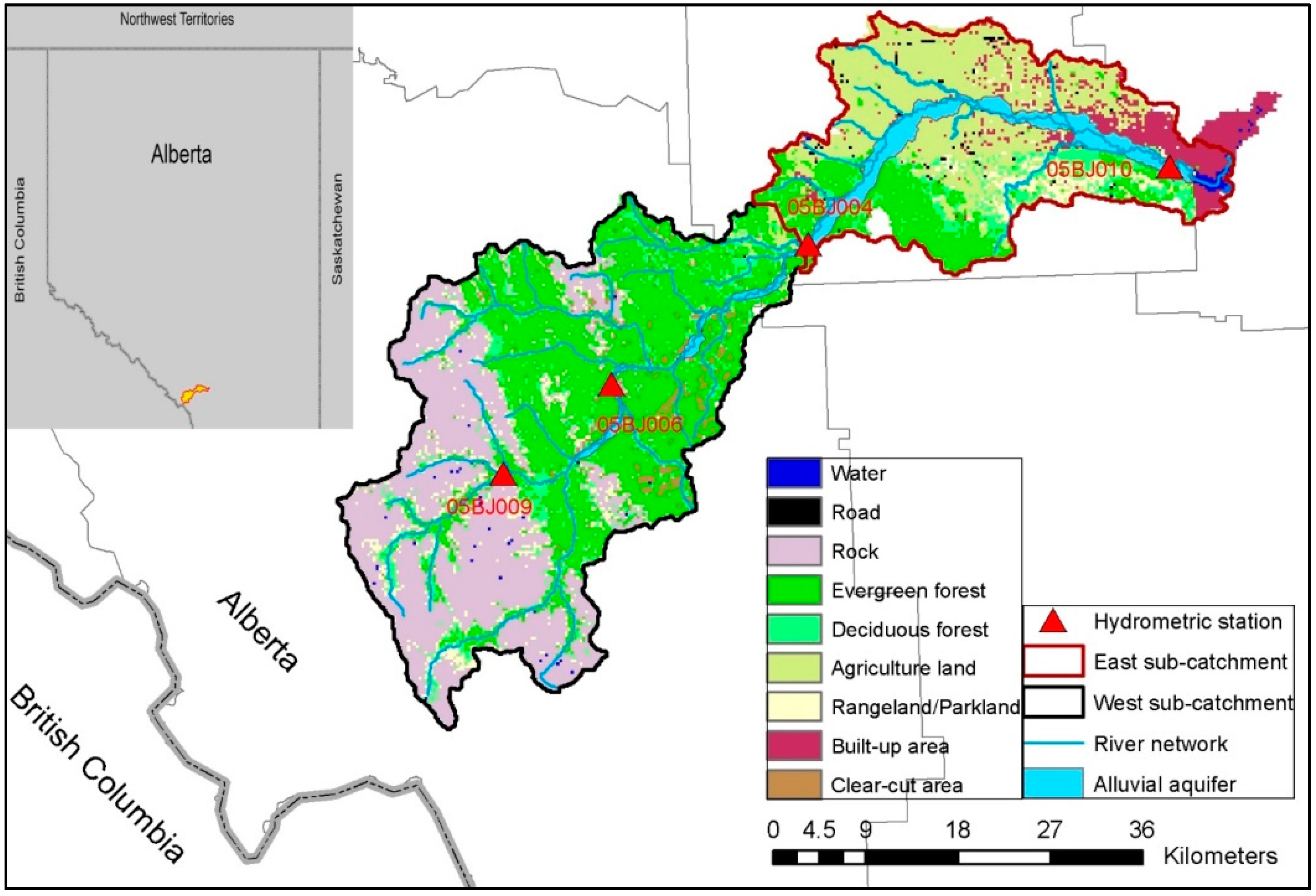
Figure 1. Location and land-use/cover of the watershed for the year 2010.
Water 09 00767 g001
Figure 2. Methodological framework of the study.
Water 09 00767 g002
Figure 3. Time periods used for the simulation of future climate change and their respective land use/cover.
Water 09 00767 g003
Figure 4. Average annual and seasonal changes in temperature and precipitation in the: 2020s (a,c,e); and 2050s (b,d,f), relative to the baseline (1961–1990).
Water 09 00767 g004
Figure 5. Average seasonal changes in evapotranspiration for the period of 2020s and 2050s, relative to the baseline (1961–1990).
Water 09 00767 g005
Figure 6. Average seasonal changes in infiltration for the period of 2020s and 2050s, relative to the baseline (1961–1990).
Water 09 00767 g006
Figure 7. Average seasonal changes in overland flow for the period of 2020s and 2050s, relative to the baseline (1961–1990).
Water 09 00767 g007
Figure 8. Average annual changes in overland flow (OL), infiltration (Inf), and evapotranspiration (ET) for the period of 2020s and 2050s, relative to the baseline (1961–1990).
Water 09 00767 g008
Figure 9. Average annual variations in streamflow in the 2020s and 2050s relative to the baseline (a,b); and percentage of streamflow that originates at the 05BJ004 station (c,d).
Water 09 00767 g009
Figure 10. Box plot of the average monthly discharge at the 0B5J004 and 05BJ010 stations.
Water 09 00767 g010
Figure 11. Average seasonal changes in streamflow for the period of 2020s and 2050s relative to the baseline (1961–1990).
Water 09 00767 g011
Figure 12. Flow duration curves for the baseline and each scenario in the 2020s and 2050s.
Water 09 00767 g012
Table 1. Measured vs. simulated streamflow during calibration and validation periods for the hydrometric stations 05BJ009, 05BJ006, 05BJ004, and 05BJ010.
ProcedureCalibration/Validation PeriodNSE (Daily)NSE (Monthly)
05B-J00905B-J00605B-J00405B-J01005B-J00905B-J00605B-J00405B-J010
Calibration1981–19910.530.630.720.630.630.750.830.75
Validation1991–2000N/AN/A0.730.71N/AN/A0.870.86
2001–2010N/AN/A0.610.63N/AN/A0.700.71