Groundwater Level Mapping Using Multiple-Point Geostatistics

Abstract

Methods based on two-point geostatistics have been routinely used to interpolate random variables such as groundwater level and concentration and to estimate their values at un-sampled locations. These methods use the observed data to analyze spatial two-point correlations and ignore the higher order moments that may play a key role in the characterization of complex patterns. In this work, a multiple-point geostatistics method is applied to interpolate groundwater level data. To do this, the ensemble simulated groundwater level maps after modeling full physics are used as training images to derive the multiple correlations. An example shows the advantages of using multiple-point geostatistics compared with the traditional two-point geostatistics methods (such as Kriging) for the interpolation of groundwater level data in a complex geological formation.

1. Introduction

Understanding the spatial and temporal variations of groundwater level is a prerequisite for groundwater resource management. In the field, groundwater level data can be obtained at monitoring wells. Interpolation methods—also referred to as geostatistics—are routinely used to estimate its values at un-sampled locations.

In geostatistics, traditional two-point variogram-based methods are commonly used to estimate the groundwater level values by analyzing the lower-order statistics of spatial distribution (i.e., covairance). For example, Theodossiou and Latinopoulos [1] employed Kriging to interpolate the groundwater level in the Anthemountas basin of northern Greece, and estimated the accuracy of interpolated values using cross-validation; Ahmadi and Sedghamiz [2] applied Kriging and co-Kriging to map the groundwater depth; Sun et al. [3] compared inverse distance weighting, radial basis function, and Kriging methods to estimate the groundwater level in a real case study, and concluded that Kriging is the optimal method for the interpolation of groundwater level in their study. In all of the applications mentioned above, two-point statistics (i.e., covariance) are used to quantify the spatial correlations, which may be inappropriate for the interpolation of the groundwater level data for complex formations such as fluvial deposition and fractured aquifers.

Multiple Points Statistics method (MPS)—which is beyond two-point statistics—has been developed to characterize complex spatial patterns in the last decade. Unlike two-point statistics methods, where correlations such as covariance are derived by fitting the experimental with the theoretical variogram, in MPS, the higher moments in particular are stored in a training image that can be obtained from the geologist and/or by analyzing outcrops; the estimation is able to mimic complex geological structures as reflected in the training image. Strebelle [4] was the first to successfully develop an algorithm (known as SNESIM) to implement MPS in an efficient way. Afterwards, a variety of algorithms have been developed to reduce the computational cost and to improve the quality of estimation. Hu and Chugunova [5] presents an overview of MPS methods.

Although MPS has been extensively studied and applied in the modeling of permeability/hydraulic conductivity, less attention has been given to the estimation/modeling of groundwater level. The main challenge resides in the acquirability of training images used in the MPS. In this work, we propose to use MPS for groundwater level mapping for the first time. To do this, we borrowed the concept of “ensemble training images”, which has been applied in the context of inverse modeling for groundwater flow and transport modeling [6], for the purpose of groundwater level estimation. In addition, we compare the results of MPS with those from two-point statistics-based methods such as Kriging in a hypothetical example, and highlight the significance using MPS for groundwater level estimation.

2. Multiple-Point Geostatistics

Unlike the SNESIM developed by Strebelle [4], which is only able to deal with categorical variables such as rock types, the MPS direct sampling method proposed by Mariethoz et al. [7] is applied to mapping continuous variables, such as groundwater level in this work. The MPS was originally developed to model formation properties such as permeability, in which case the training image could be a conceptual model of modeled aquifer. However, when the groundwater level is considered as a random variable, the salient question is how to find its training image. Thus, the concept of “ensemble training images” proposed by Zhou et al. [6] is utilized here. Specifically, the simulated groundwater level maps after modeling the full physics are used as the training images for the estimation.

In the direct sampling method, the pattern (i.e., data event) is composed of the measured data as well as the previously estimated values, and the matched pattern is found by scanning the whole training images. In light of considering the ensemble training images for groundwater level mapping, the algorithm can be listed as the following steps:

• Generate the hydraulic conductivity realizations using multiple-point geostatistics.
• Run forward modeling such as MODFLOW to get the simulated groundwater level maps that will subsequently be used as the training images for the conditional simulation.
• Apply direct sampling MPS to simulate the groundwater level maps, given the measured data.

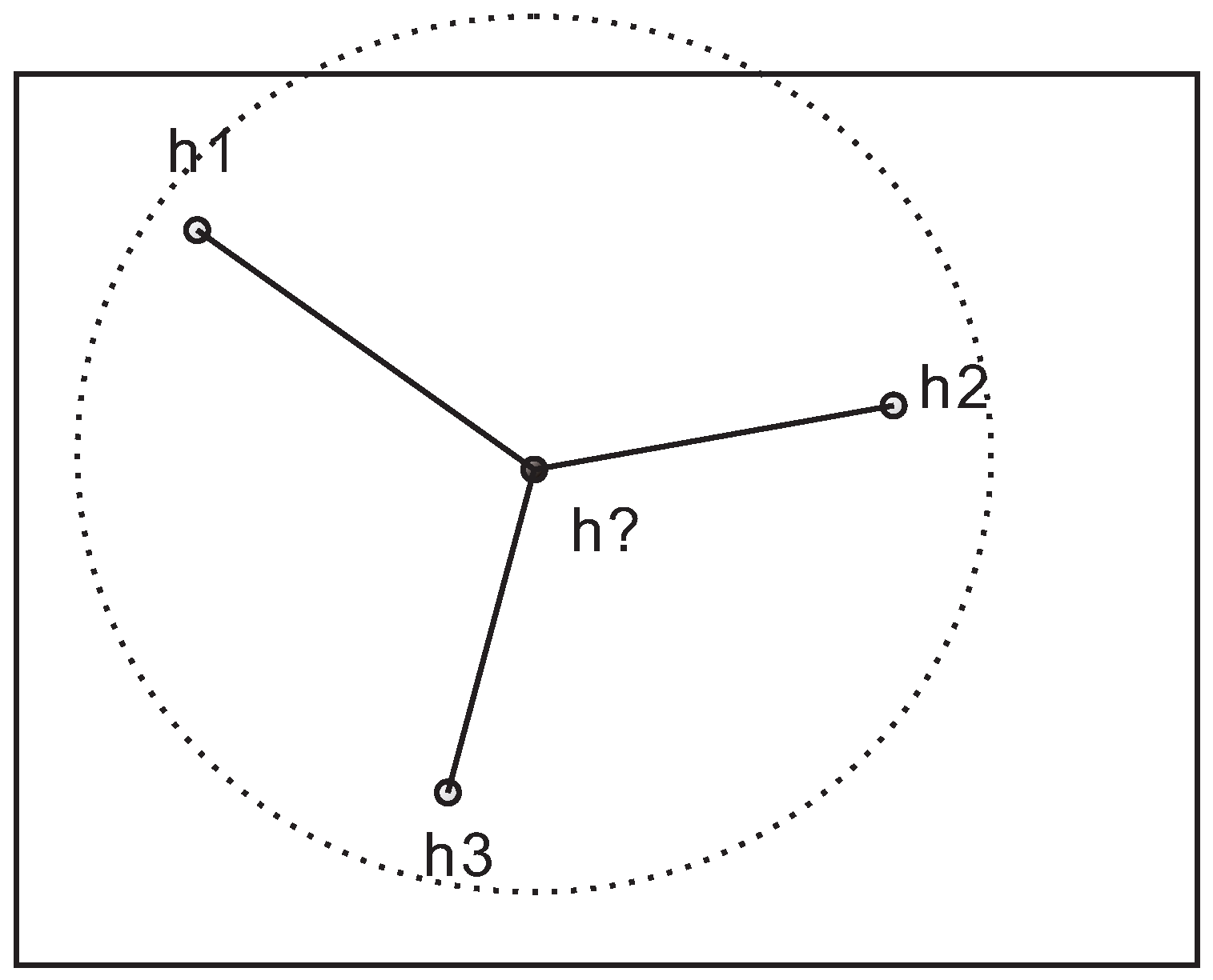
  • Configure the conditional pattern ($\mathbf{P}$) that is composed of measured groundwater level data and the previously simulated ones (see Figure 1). Assuming that the total number of elements in the pattern is m, the pattern for the grid block i and realization j will be

    $${\mathbf{P}}_{i,j}=[\begin{array}{c}{h}_1,h_2,\cdots ,h_m\end{array}{]}_{i,j}$$

    (1)
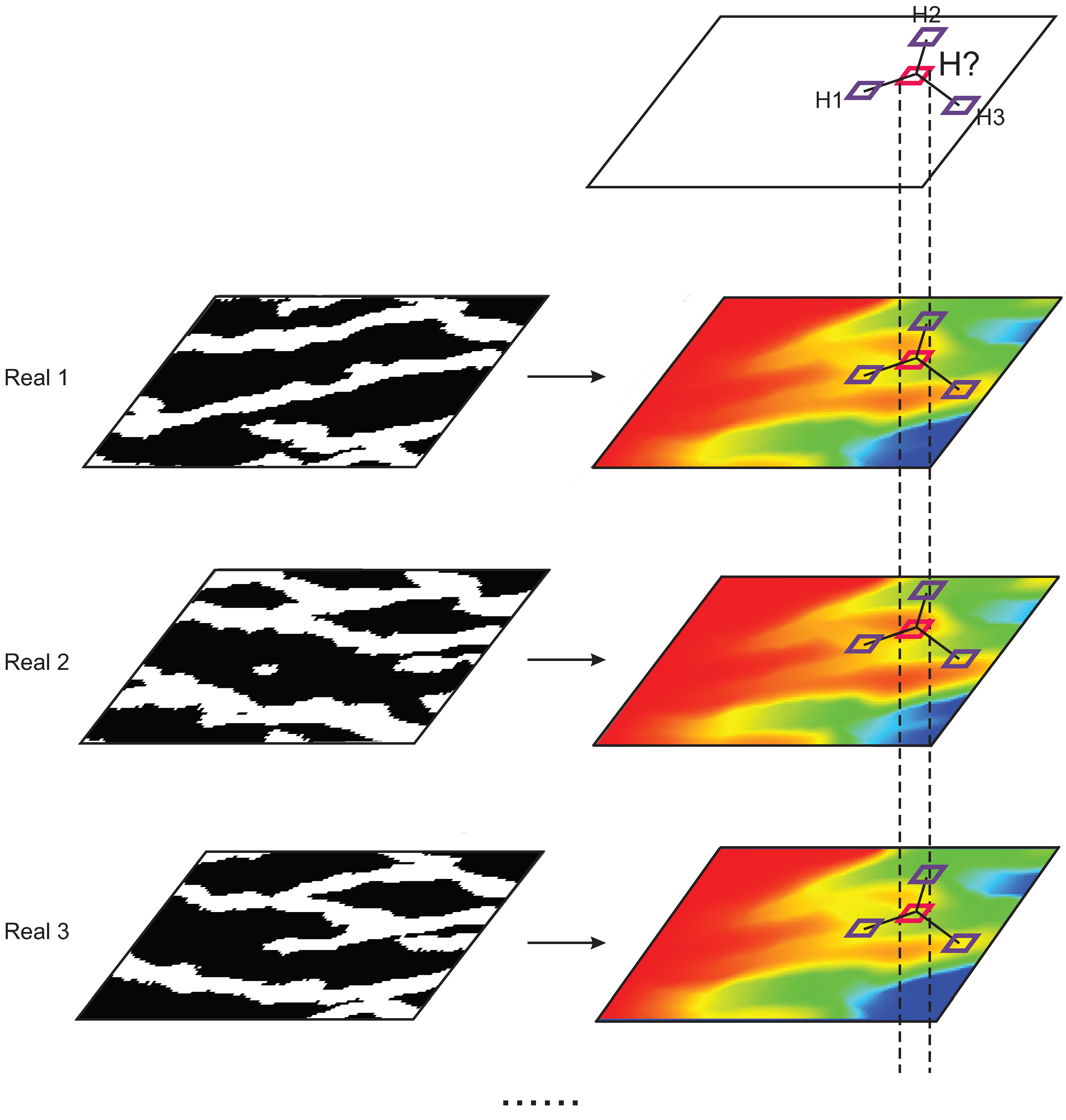
  • Center on the estimated node, and vertically scan the ensemble training images to find candidate patterns ($\tilde{\mathbf{P}}$) (see Figure 2). Since groundwater level is a continuous variable, an exact match almost could not be found. Therefore, distance is used to quantify the dissimilarity between the conditional and candidate patterns. A lesser distance value means much more similarity of patterns. The weighted Euclidean distance function is employed to calculate the distance,

    $$d_{(\mathbf{P},\tilde{\mathbf{P}})}=\sqrt{\frac{1}{{\sum }_{i=1}^m{h}_i^{-1}}\sum _{i=1}^m{h}_i^{-1}\frac{{(\mathbf{P}-\tilde{\mathbf{P}})}^2}{d_{max}^2}}$$

    (2)

    where h is the Euclidean distance between the grid block to be simulated and the conditioning data, and $d_{max}$ is the maximum absolute difference of heads observed in the pattern.
  • Accept or reject the candidate pattern. If the calculated distance is smaller than the predefined tolerance value, accept this candidate pattern and copy the groundwater level from the training image to the estimated grid block. Otherwise, the distances between the conditional and other candidate patterns are computed until all the training images are visited. The conditional pattern with the smallest distance will be kept, and the corresponding groundwater level will be pasted to the estimated grid block.
  • Repeat the above process until the groundwater levels at all grid blocks are estimated.

The simulated groundwater level map will condition on measured data, and honor the higher order moments that are implicitly saved in the training images. By changing the visiting path of the grid block in each realization, the multiple realizations of groundwater level will be reached, and can be used to quantify the uncertainty.

There are two remarkable features of modeling groundwater level which are different from the modeling of formation properties using MPS. First, the ensemble training images are derived from the simulation of full physics that requires the initialization of parameters such as hydraulic conductivity. Secondly, the groundwater level, as a non-local variable, is dependent on the source/sinks and boundary conditions, which calls for the scanning of candidate patterns at a fixed location through the ensemble.

Notice that the groundwater level estimation in the framework of MPS needs a definition of pattern that quantifies the multiple correlations of the groundwater level data, and the estimated value is directly sampled from the training image. This procedure ensures the reproduction of complex patterns as in the training images. However, in two-point statistics such as Kriging, only lower-order moments (i.e., mean and covariance) are taken into consideration, and it is commonly insufficient to characterize the complex structures.

3. Example

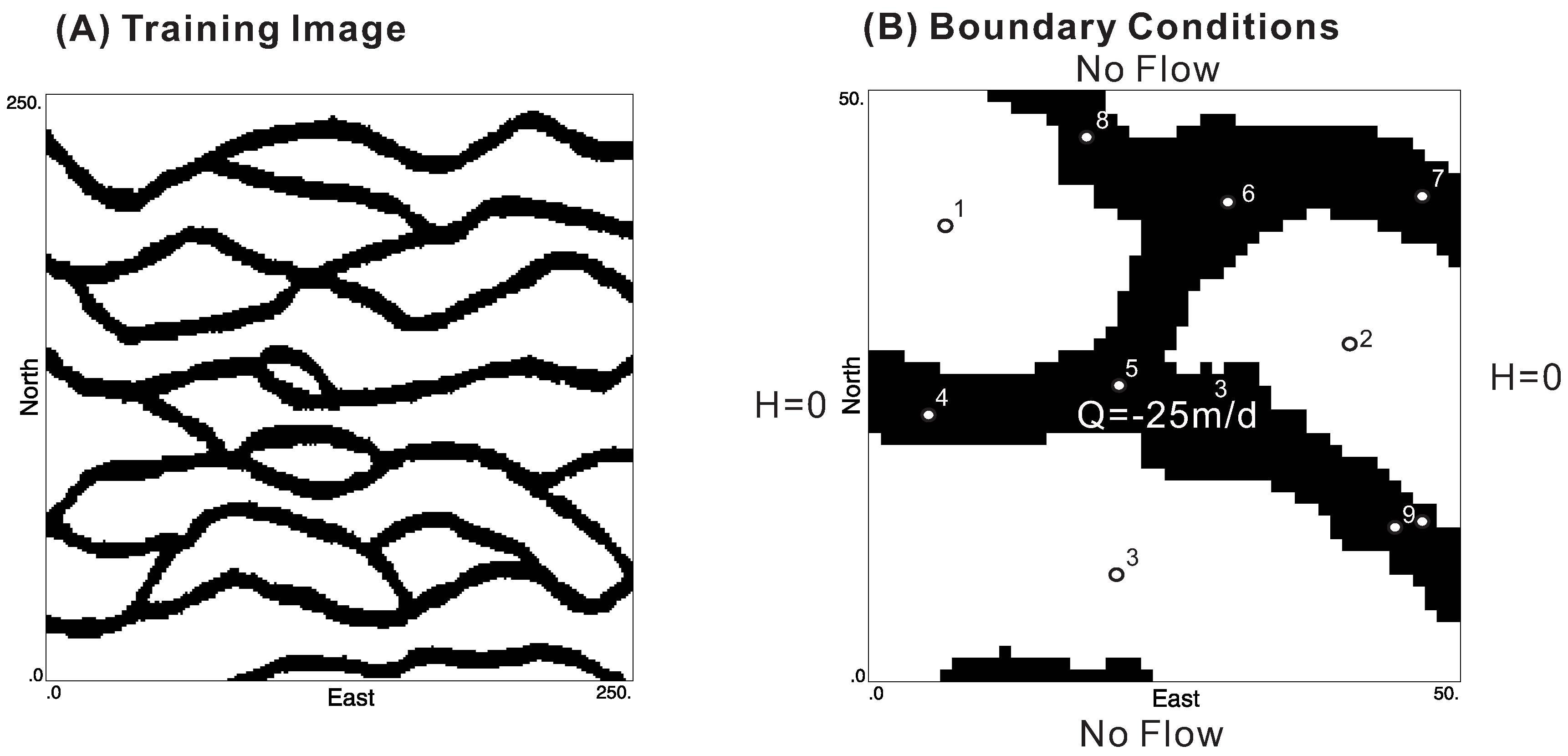
A hypothetical bimodal aquifer that is composed of sand and shale facies is used to demonstrate the effectiveness of the proposed method. The aquifer is discretized into 50 × 50 × 1 cells with cell size 1 m × 1 m× 1 m. The reference facies field is generated by direct sampling MPS method [7], using the training image from Strebelle [4] (see Figure 3). Constant hydraulic conductivities equal to 10 and ${10}^{-4}$ m/d are assigned to sand and shale, respectively.

The aquifer is assumed to be confined with impermeable boundaries in the north and south, with constant head boundaries (i.e., h = 0 m) in the east and west. A pumping well with a constant flow rate of 25 ${\mathrm{m}}^3/\mathrm{d}$ is located at the center of aquifer. There are eight observation wells. The initial head over the domain is 0 m. Specific storage is assumed constant and equal to 0.01 ${\mathrm{m}}^{-1}$. The groundwater flow equation is solved for the reference field using MODFLOW [8]. 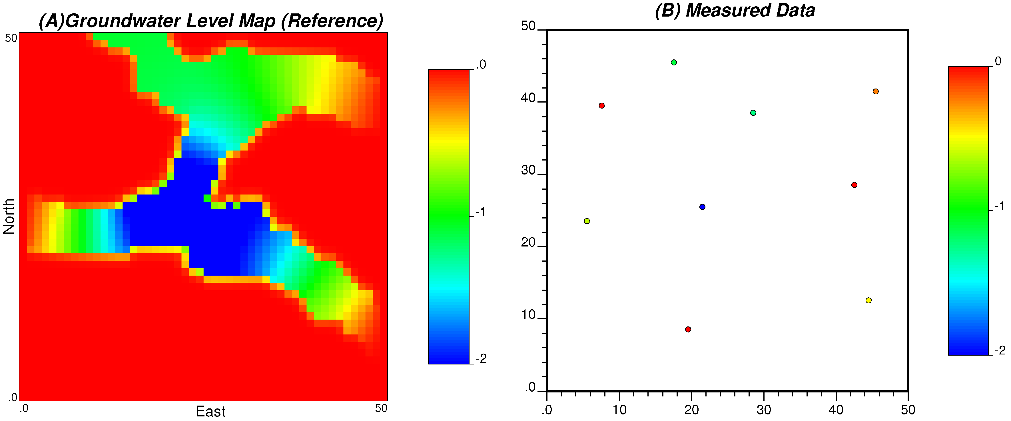The simulated groundwater level at time (t = 1.3 days) will be assumed as the “true” map (see Figure 4). Then, the groundwater level data are collected for nine wells and will be used as measured data for the interpolation.

As mentioned in the previous section, ensemble training images of groundwater levels are needed for the groundwater level mapping in the framework of MPS. Thus, 500 hydraulic conductivity realizations are generated using direct sampling MPS method, which will subsequently be fed to the flow simulation. The major parameters used in the direct sampling MPS are listed as follows: the maximum search radius is set at 10 m, the maximum number of conditioning data in the pattern is fixed at 10, and the distance tolerance for the groundwater level pattern is 0, in order to find best matched patterns—although a larger computational cost may be involved. The role of these parameters in the implementation of MPS can be found in the study by Li et al. [9].

The objective of this exercise is to map the groundwater level at un-sampled locations based on measurement data, using MPS method. To highlight the significance of MPS method on the mapping of groundwater level in complex formations, the commonly used two-point statistics-based method Kriging is also implemented and compared with the MPS method using the same conditioning data set. It is worth pointing out that, for the case of Kriging, no ensemble training images and flow simulations are required; conversely, two-point statistics (such as covariance) are needed for the estimation, which can be achieved by analyzing the variogram on the data set [10].

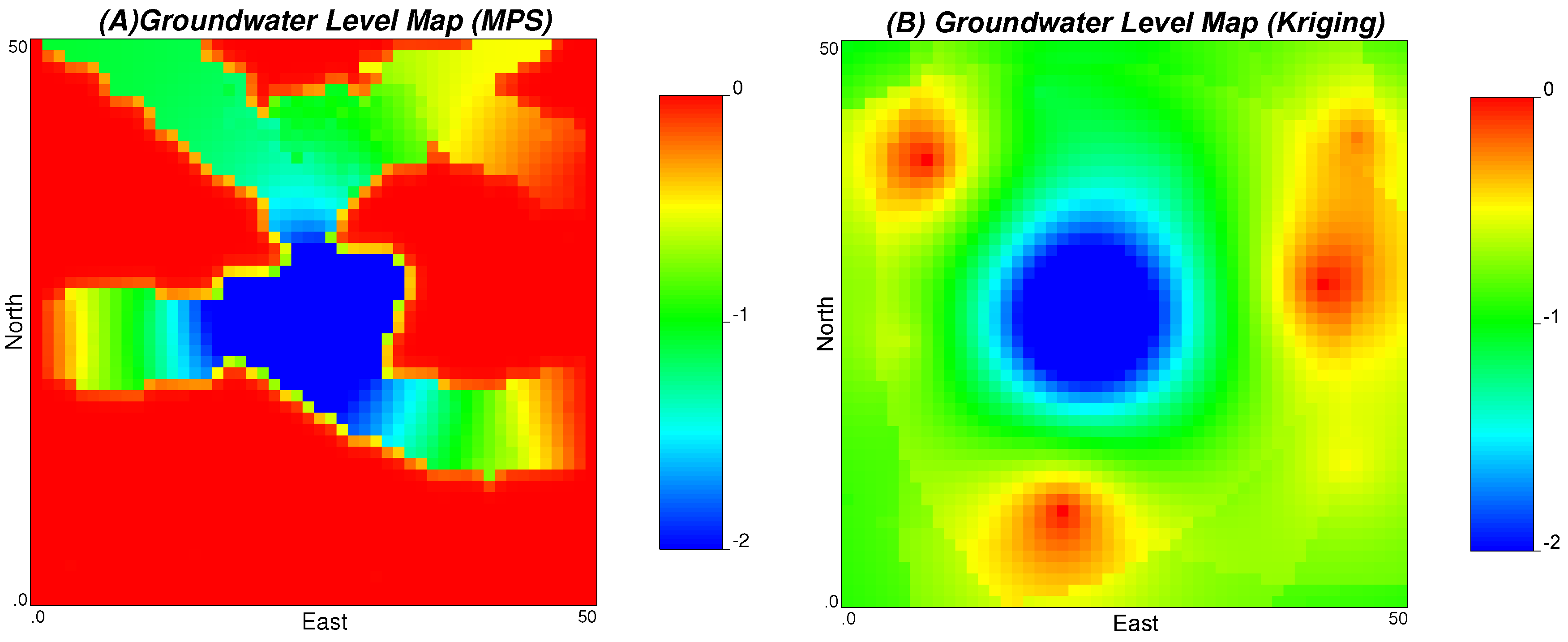
Figure 5 displays the results of groundwater level mapping using MPS and Kriging methods. Obviously, the simulated groundwater level map using MPS exhibits similar patterns to the “true” map, while the one using Kriging shows a smoothed groundwater level map. In essence, the success of the former approach resides in the integration of hydraulic conductivity on the mapping of groundwater level. In other words, the ensemble training images of groundwater level simulated from hydraulic conductivity make the multiple-point statistics simulation possible. However, the latter only considered the two-point spatial correlations within the data and could not simulate the complex patterns as in the reference.

Apparently, the computational cost of the MPS method for the interpolation of groundwater level is much higher than that of Kriging, where no forward modeling is needed. However, a much higher accuracy is achieved using MPS, to reproduce the spatial patterns that are of importance to understand the flow and solute transport behavior. Therefore, in the real-world settings, there is a trade-off between cost and accuracy for selection of an effective interpolation method that works best for the specific site.

Note that the groundwater mapping method using MPS needs the ensemble training images that might be computationally expensive to be acquired in real case studies. Reducing the computational cost by using proxy models or other alternative methods for the generation of training images will be explored in future works.

4. Summary

In the last two decades, traditional two-point geostatistics (such as Kriging) have been routinely used to interpolate groundwater level data, in order to estimate the values at un-sampled locations. However, it is evident that two-point geostatistics methods are inappropriate for complex aquifers where the groundwater level may show complex patterns. These patterns are significant for water resource management. Multiple-point geostatistics methods provide an avenue to simulate curvilinear structures. MPS has been applied in many areas, such as hydraulic conductivity modeling and rainfall history reconstruction. However, few studies focus on the estimation of groundwater level and concentration. The main challenge is to find the corresponding training image for the learning procedure. In this work, the ensemble training images simulated from hydraulic conductivity are applied as the basis for the MPS modeling of groundwater level. In the example, the results show that the MPS better reproduces the patterns of groundwater level than Kriging, a two-point geostatistics method. Through the course of this comparison, it became clear that the use of two-point geostatistics for groundwater level mapping should be done with caution. In terms of methodology, the MPS method is general and could be applied for the interpolation of other random variables, such as concentration.

References

- Theodossiou, N.; Latinopoulos, P. Evaluation and optimisation of groundwater observation networks using the kriging methodology. Environ. Model. Softw. 2006, 21, 991–1000. [Google Scholar] [CrossRef]
- Ahmadi, S.H.; Sedghamiz, A. Application and evaluation of kriging and cokriging methods on groundwater depth mapping. Environ. Monit. Assess. 2008, 138, 357–368. [Google Scholar] [CrossRef] [PubMed]
- Sun, Y.; Kang, S.; Li, F.; Zhang, L. Comparison of interpolation methods for depth to groundwater and its temporal and spatial variations in the minqin oasis of northwest china. Environ. Model. Softw. 2009, 24, 1163–1170. [Google Scholar] [CrossRef]
- Strebelle, S. Conditional simulation of complex geological structures using multiple-point statistics. Math. Geol. 2002, 34, 1–21. [Google Scholar] [CrossRef]
- Hu, L.; Chugunova, T. Multiple-point geostatistics for modeling subsurface heterogeneity: A comprehensive review. Water Resour. Res. 2008, 44. [Google Scholar] [CrossRef]
- Zhou, H.; Gómez-Hernández, J.J.; Li, L. A pattern-search-based inverse method. Water Resour. Res. 2012, 48. [Google Scholar] [CrossRef]
- Mariethoz, G.; Renard, P.; Straubhaar, J. The direct sampling method to perform multiple-point geostatistical simulations. Water Resour. Res. 2010, 46. [Google Scholar] [CrossRef]
- Harbaugh, A.W.; Banta, E.R.; Hill, M.C.; McDonald, M.G. MODFLOW-2000, the U.S. Geological Survey Modular Ground-Water Model; U.S. Geological Survey, Branch of Information Services: Reston, VA, USA; Denver, CO, USA, 2000.
- Li, L.; Srinivasan, S.; Zhou, H.; Gómez-Hernández, J.J. A pilot point guided pattern matching approach to integrate dynamic data into geological modeling. Adv. Water Resour. 2013, 62, 125–138. [Google Scholar] [CrossRef]
- Gómez-Hernández, J.J.; Journel, A.G. Joint sequential simulation of multigaussian fields. In Geostatistics Troia92; Springer: Dordrecht, The Netherlands, 1993; pp. 85–94. [Google Scholar]
© 2016 by the authors; licensee MDPI, Basel, Switzerland. This article is an open access article distributed under the terms and conditions of the Creative Commons Attribution (CC-BY) license (http://creativecommons.org/licenses/by/4.0/).