Article

Evaluation of Soil Water Availability (SWA) Based on Hydrological Modelling in Arid and Semi-Arid Areas: A Case Study in Handan City, China

1
Institute of Soil and Water Conservation, Northwest A&F University, Yangling 712100, Shaanxi, China
2
Institute of Water Saving Agriculture in Arid Regions of China, Northwest A&F University, Yangling 712100, Shaanxi, China
3
State Key Laboratory of Simulation and Regulation of Water Cycle in River Basin, China Institute of Water Resources and Hydropower Research, Beijing 100038, China
*
Author to whom correspondence should be addressed.
Water 2016, 8(8), 360; https://doi.org/10.3390/w8080360
Submission received: 22 May 2016 / Revised: 8 August 2016 / Accepted: 12 August 2016 / Published: 22 August 2016

Abstract

:
To evaluate the spatial and temporal soil water availability (SWA) and improve the soil water use efficiency in agriculture, this study established a new index system for SWA evaluation considering the soil storage capacity, the temporal and spatial matching degree between soil water supply and crop water demand, and the soil water transformation and utilization efficiency. To quantitatively calculate the indexes, a self-developed hydrological model (MODCYCLE) was introduced and applied in Handan City. The results show that MODCYCLE performed well in simulating the soil hydrological processes. A comparison of the observed soil moisture data and the simulated values revealed relative errors below 10% and correlation coefficients all above 0.7. According to the evaluation results, the SWA for different typical years was very unevenly distributed in Handan City. The average SWA in a normal year is 0.71, which is higher than that in dry years at 0.62 and in wet years at 0.65. Regarding different regions, the average SWA was generally much higher in the eastern plain area than that in the western mountainous area. Generally, there is a great potential for improving SWA and further the sustainable development of soil water resource, particularly for dryland farming in similar areas.

1. Introduction

Influenced by both climate change and high-intensity human activities, the volume of runoff water resources is currently decreasing sharply [1]. Under this background, water use competition among different sectors (e.g., urban, industry, agriculture, and ecology) is increasing. The agriculture sector is known to be vulnerable compared with other sectors that have better economic benefits [2]. Therefore, agricultural water resources are largely diverted to other sectors to pursue higher benefits. This practice is definitely a great threat to grain production and food security. To guarantee sustainable agricultural development and to promote food security, an increasing number of studies have focused on soil water resources, particularly in arid and semi-arid areas. In general, water can be directly absorbed by crops and plants after it is transformed into soil moisture. Therefore, soil water, as a type of water resource, plays an important role in agricultural production and food security. However, agricultural specialists and water resource managers have traditionally paid much attention to the “visible” water, e.g., surface water and ground water, which is also known as blue water. Owing to the difficulty of monitoring and regulating soil water, the utilization value of soil water resources is largely ignored, particularly in Chinese agriculture. Recently, soil water monitoring and simulation technologies have developed significantly, which has provided a good foundation for the efficient use and management of soil water resources in rain-fed agriculture, particularly in arid and semiarid areas.
Soil moisture, known as a direct index of soil water availability (SWA), is an important indicator for farmland hydrological forecasts and irrigation scheduling. Therefore, most previous studies have focused on the monitoring and forecasting of soil moisture by using different techniques. Robinson et al. [3] concluded that there are two main approaches for studying the spatial–temporal distribution of soil moisture. The first method refers mainly to measurement methods by direct contact with the soil profile, such as gravimetric methods [4], tensiometers [5], the neutron probe method [6], and time domain reflectometry (TDR) [7,8]. Tanaka and Aase [9] used the neutron scattering technique to measure soil moisture at the field scale to determine the season in which the fallow method might influence soil water storage. Zegelin et al. [10] improved the field probes to detect the soil water content based on TDR, which has been widely used owing to its convenience and economic efficiency. Gao et al. [11] studied the spatial variability of the root zone soil moisture (RZSM) in gullies by using the observed soil moisture data collected by the TDR method from nearby uplands. The soil moisture data collected by the traditional direct methods are accurate but are time-consuming and cost intensive if the sampling area is large [12].
The second method, which refers mainly to remote sensing techniques [13], cannot directly measure the RZSM. However, it can sense the RZSM without direct contact with the soil based on multi-spectral information from the soil layer. Remote sensing methods include passive microwave radiometers, synthetic aperture radars, scatterometers, and thermal methods. These methods are either ground based or operated from airborne or spaceborne platforms [14]. Recent progress in remote sensing technologies has allowed us to obtain frequent soil moisture distribution maps easily and quickly [15,16]. Kong and Dorling [17] retrieved near-surface soil moisture from advanced synthetic aperture radar imagery, which showed satisfactory accuracy for the shallow soil layer profile. Ford et al. [18] used an exponential decay filter to estimate RZSM using the near-surface soil moisture derived from the Soil Moisture and Ocean Salinity (SMOS) satellite. Martínez-Fernández et al. [19] calculated the soil water deficit index (SWDI) based on SMOS satellite remote sensing data for agricultural drought monitoring. The advantage of remote sensing is that it gives uniform spatial and temporal coverage of the estimated soil moisture easily and quickly. However, the limitations include confinement to the top few centimetres of the soil layer and coarse spatial and temporal resolutions. However, when integrated with a land surface process model, remote sensing can estimate the soil moisture both at the surface and deep in the root zone with high spatial and temporal resolutions. In addition, data assimilation provides a means for combining the advantages of modelling with those of remote sensing data. A host of studies based on remote sensing measurement have used data assimilation to derive an indirect estimate of the RZSM [20]. Montaldo and Albertson [21] developed a multi-scale assimilation approach for RZSM estimation, which is shown to provide marked improvements. Reichle and Koster [22] assimilated the Scanning Multi-channel Microwave Radiometer (SMMR)-derived real surface soil moisture data into the National Aeronautics and Space Administration (NASA) Catchment land surface model at a large continental scale over a long period. The soil moisture estimates in this research are significantly better than those obtained with the model or from the satellite alone. Moreover, using statistical and distributed hydrological models to simulate the spatial and temporal pattern of soil water has become an attractive method because it is more time saving and cost effective than traditional methods. Kim [23] developed a time series model for soil moisture simulation and the results showed that the simulated values fit well with the observed soil moisture series. Gao et al. [24] mapped the spatial and temporal distribution of soil water moisture based on a self-developed hydrological model in Northern China. The physical-based distributed hydrological model showed good reliability for soil moisture simulation.
The studies mentioned above focus mainly on soil water observation, soil moisture mapping, and agricultural drought monitoring. Few scientists have sought to improve soil water use efficiency based on soil water content observation and simulation for agricultural water management. In the context of climate change and strong anthropogenic influence on the hydrological cycle, the available volume of blue water resources is shrinking significantly. Therefore, improving the utilization efficiency of green water resources and making full use of soil water resources in agriculture are of great concern, particularly in arid and semi-arid areas. It is widely accepted that evaluation of soil water resources availability is the first and most important step for high-efficiency soil water resources development and sustainable utilization. Therefore, the objective of this study is to introduce a distributed hydrological model to depict the soil water transformation and flow routes at a regional farmland scale. The soil water availability assessment index system is established to jointly consider factors such as soil storage capacity, soil water recharge and discharge rates, and soil water uptake efficiency by crops and plants. The main objectives of this study include (1) development of a spatially distributed hydrological model to simulate the soil water transformation and flow process based on the complex tillage and water management regimes of farmland in the North China Plain; (2) establishment of the soil water availability assessment index framework considering such parameters as soil properties, soil water reservoir characteristics, and soil water recharge and discharge efficiency; and (3) selection of Handan City in the North China Plain in a semi-arid area as the study region and quantitative calculation of the farmland soil water availability. In addition, we reveal the spatial and temporal variability of soil water use potential and efficiency in accordance with the evaluation results, and we provide specific and differential suggestions and strategies for different sub-regions in the study area. This study can serve as a guide for improving soil water use efficiency and maintaining sustainable agricultural and ecological development in arid and semi-arid areas.

2. Materials and Methods

2.1. Soil Water Simulation Tool

Before SWA evaluation is conducted, the scientist should understand the soil water movement process in the farmland that is used to quantify the water availability index. However, for a large-scale basin or region, it is impossible to explore the soil water movement process though field experiments, which are time consuming and cost intensive. With the development of computer numerical simulation technology, the soil transformation and flow process at a large scale has been efficiently simulated by hydrological models in many studies [25]. In this study, the object-oriented modularised model for basin-scale water cycle simulation (MODCYCLE) is introduced to simulate the farmland hydrological processes and to map the temporal and spatial distribution of the farmland soil water moisture [24,26]. MODCYCLE, self-developed by the China Institute of Water Resources and Hydropower Research (IWHR), is a spatially distributed model properly combining a hydro–physical model with a conceptual model. Moreover, MODCYCLE avoids the difficulty in parameterization and overload of computation.
MODCYCLE is similar to the commonly used soil and water assessment tool (SWAT) model [27], particularly in its hydrological modelling and calculation. Both are semi-distributed and conceptual–physical models in which the main hydrological processes such as overland runoff, groundwater runoff, evapotranspiration, soil water infiltration, and percolation are all depicted with generalised physical methods and simplified empirical formulas. Numerous previous studies have proved that SWAT is an effective tool for simulating soil moisture distribution at the regional scale, particularly in natural basins or areas of limited anthropogenic influence [28,29]. However, it performs poorly when simulating the hydrological processes in areas influenced by strong human activities, especially for the complex cropping systems and irrigation regimes in China. Therefore, MODCYCLE is designed to improve the simulation accuracy under the conditions of strong anthropogenic influences and complicated Chinese tillage systems. According to the simulation principle, MODCYCLE uses the core of SWAT because the simulation principles of SWAT are proven to be effective and practical by a series of case studies and applications. Moreover, a special module, the agricultural management module, has been embedded in MODCYCLE to depict the complex hydrological processes of Chinese farmland with complicated tilling practices and strong anthropogenic influences. Based on the agricultural management module, an agricultural activity command database in accordance with the current farmland management regimes of China has been created, which controls MODCYCLE to precisely and elaborately simulate the farmland hydrological processes. In summary, compared with SWAT, MODCYCLE performs much better in depicting the farmland soil water movement processes in China. Therefore, it was used as an important tool for SWA evaluation in this study.
The structural framework of MODCYCLE is similar to that of SWAT, the most widely used hydrological model. The first step in MODCYCLE is to divide the study area into sub-basins. The sub-basins are further subdivided into different hydrological response units (HRUs). The runoff generated in each sub-basin is from two sources: the area within the sub-basin and the upstream contributing areas. Based on a digital elevation model (DEM) and GIS analysis, the topological relationships among the sub-basins are established, and the runoff flow directions in the sub-basin can be depicted. For SWA evaluation, soil water movement simulation is of extreme importance. Water molecules are absorbed in the soil mass forced by the soil matric potential in an unsaturated zone. Therefore, soil water moves much slower than surface water. However, compared with soil water movement in a horizontal direction, the speed in the vertical direction is much faster because of gravity. As a result, soil water movement in the horizontal direction in an unsaturated zone can be neglected, although that in the vertical direction must be considered. In MODCYCLE, the main hydrological process in the vertical direction is simulated through a one-dimensional (1D) Soil Column Method at the HRU scale (Figure 1).
As shown in Figure 1, HRU is regarded as the basic simulation unit in the model. Vertical water movement consists of three processes: the surface water process, soil water process, and ground water process. Because the soil water process is the main concern in our study, the simulation method for soil water movement is introduced in detail below. In the 1D soil column, the soil layer is divided into two parts. The upper part is the schematised layer, and the lower part is the seepage transition layer, as shown in Figure 1. Ordinarily, the schematised layer is the crop root zone in farmland, where the soil water content fluctuates frequently at different timescales, particularly in the growing season. To precisely simulate the soil water content variation process in the crop root zone, the schematised layer should be also subdivided into different sub-layers (e.g., Layer A, Layer B, Layer C, etc.). In MODCYCLE, the schematised layer can be subdivided into 10 multiple soil layers. The seepage transition layer is directly beneath the schematised layer, where the soil water content is relatively stable. However, the seepage transition layer is an important linkage zone for water exchange between the ground water and soil water. That is, the seepage transition layer is a buffer zone in which the surplus water can be stored during the wet season and is supplied into the soil root zone for crop growth during the dry season. Therefore, the seepage transition layer plays a significant role in farmland cultivation and management. In the 1D soil column method, the water balance equation can be described as
Δ S W = R + I R + G E V S F Δ L F U E V P E V S E V S E P
where Δ S W is the change in the soil water content in the simulation period, R is the equivalent precipitation depth adjusted for canopy interception, I R is the irrigation depth in the simulation period, G E V is the evaporation depth from phreatic water to the crop root zone, S F is the surface runoff loss depth, Δ L F is the change in the surface water ponding depth, U E V is the evaporation depth from the surface water, P E V is the crop evapotranspiration depth, S E V is the evaporation depth from the soil layer, and S E P is the water deep infiltration depth from the soil layer to the groundwater aquifer; all are in millimetres. As described in Equation (1), the entire soil layer can be considered as a water tank. Most processes of water exchange in the soil layer occur through the top boundary (farmland surface) and the bottom boundary (ground water table). Nine variables need to be determined to solve the equation. R and I R are input parameters in the model, and the calculation methods for the rest of the parameters can be obtained from related studies [26,30].

2.2. Soil Water Availability Evaluation Method

2.2.1. Definition of Soil Water Availability

Improving the efficiency of agricultural water resources is the central topic for water-saving agriculture technologies. In arid and semi-arid areas, any type of water resource should be transformed into soil water before it is effectively absorbed and utilised by crops and plants. Based on the analysis of soil water resource properties, this study argues that three factors will primarily influence soil water use efficiency at the farmland scale. The first is availability of the soil water quantity, which is mainly affected by soil particles and root zone depth. Not all water stored in the soil layer can be directly absorbed by crops; essentially, only the soil moisture above the wilting point and below the field capacity can be used by crops. Here, we introduce two first-class indices to represent the soil water quantity: soil water storage capacity [31] and the operational characteristics of the farmland soil reservoir [32], the calculation methods of which will be introduced later. The second factor is the matching degree of soil water resources between the supply and demand. In some cases, although there is sufficient soil water supply throughout the year, the crops may also suffer from drought in some months (e.g., April and May) because the temporal distribution of available soil water is uneven. Here, we introduce one first-class index to represent the matching degree of the soil water resource, which includes two sub-indices: the temporal matching degree index and the spatial matching degree index. The third factor is the efficiency of soil water transformation and uptake by plants. Here, we introduce one first-class index to represent the soil water efficiency [33,34], which also includes two sub-indices: soil water conversion efficiency and crop absorption efficiency. The details of the aforementioned indices are given in Table 1.
Previous studies have largely examined how to increase the efficiency of soil water transformation and plant absorption. However, they neglect to discuss the importance of the availability and quantity of soil water to be used by plants and crops and the degree of temporal and spatial matching degree between the soil water supply and the demand. In this study, we comprehensively consider these three factors and suggest a new concept for SWA evaluation. An optimal objective function is presented to quantitatively characterise the soil water availability at the farmland scale, as shown in Equation (2):
U = F ( A , R , E )
where U represents the comprehensive SWA, F ( X , Y , Z ) is the soil water availability evaluation function, A represents the factor for the degree of difficulty of the soil water to be used by plants and crops, R represents the factor for the degree of matching between the soil water supply and the water demand, and E represents the factor for the efficiency of soil water transformation and plant uptake.

2.2.2. Framework of the Soil Water Availability Index System

As shown in Equation (2), the optimal objective function of soil water availability is only a conceptual expression and it cannot be used to quantitatively evaluate the soil water availability directly. Therefore, an index system was introduced to quantitatively characterise the three factors. Based on the index system, we used the analytic hierarchy process (AHP) method to calculate the comprehensive SWA.
The SWA index system, presented in Table 1, includes four first-class indices and seven second-class indicators. The first and second first-class indices (C1 and C2) mainly represent the factor for the degree of difficulty for the soil water to be used by plants and crops, which are further subdivided into three second-class indicators. The third first-class index (C3) represents the matching degree between the soil water supply and the water demand, which is further subdivided into two second-class indicators. The fourth first-class index (C4) represents the factor for the efficiency of the soil water transformation and plant absorption, which is further subdivided into two second-class indicators.

Index for Soil Water Storage Capacity (C1)

Soil water storage is a key parameter for farmland hydrology in arid and semiarid areas. In view of the water holding ability of the soil, scientists always regard this capacity as the soil water reservoir capacity. According to previous studies [31], soil water reservoir capacities include mainly the total soil water reservoir capacity (TC), soil water storage capacity (SC), unavailable soil water reservoir capacity (UC), available soil water reservoir capacity (AC), and soil dead water storage capacity (DC). In this study, we present a second-class index (C11) to represent the first-class index soil water storage capacity (C1). Here, C11 represents the available soil water reservoir capacity, which is essentially determined by the soil properties in the root zone of the farmland. With a total of n soil layers in the root zone, the valid capacity of the soil reservoir can be represented as
W p = i = 1 n ( FC ( i ) θ wp ( i ) ) · D i
where W p represents the valid storage capacity (equivalent water depth) of the soil water in the crop root zone; F C ( i ) represents the field soil water holding capacity (equivalent water depth) of the soil layer i ; θ w p ( i ) is the volume of the soil water (equivalent water depth) at the wilting point of the soil layer i , and D i represents the thickness of the soil layer i , all of which are in millimetres. In addition, n represents the number of soil layers in the root zone.

Index for the Operational Characteristics of the Farmland Soil Reservoir (C2)

To characterise the average soil water shortage severity in the soil root zone within one year, the two second-class indices (C21 and C22) are introduced to represent the index for the operational characteristics of the farmland soil reservoir. The index C21 is the average value of the annual empty storage capacity of the soil reservoir:
W e ¯ = ( j = 1 m i = 1 n ( ( FC ( i ) θ j ( i ) ) · D i ) ) / m
where W e ¯ is the average value of the annual empty storage capacity (equivalent water depth) of the soil reservoir, in millimetres; F C ( i ) represents the field soil water holding capacity (equivalent water depth) of the soil layer i , in millimetres; θ w p ( i ) represents the actual soil water content (equivalent water depth) of the soil layer i ; D i represents the thickness of the soil layer i , in millimetres; m represents the total number of days in the evaluation period; and n represents the number of layers of soil in the root zone.
The index C22 represents the average annual variation of the empty storage capacity of the soil reservoir for the root zone:
C w = j = 1 m ( i = 1 n ( ( FC ( i ) θ j ( i ) ) · D i ) W e ¯ ) 2 m / W e ¯
where C w is the average annual variation of the empty storage capacity of the soil reservoir, in millimetres. The other terms are the same as those described in Equation (4).

Index of Degree of Matching between the Soil Water Supply and Crop Water Demand (C3)

In this study, the two second-class indexes (C31 and C32) were originally introduced to characterise the matching degree between the soil water supply and crop water demand. The index C31 represents the temporal matching degree between the soil water supply and crop water demand:
m ti = { e RC i DE i IR i DE i ,   if   RC i DE i IR i < 0 1   , if   RC i DE i IR i 0
m t = i = 1 n m ti n
where m t i represents the temporal matching degree between the soil water supply and crop water demand in month i in the growing period, with values ranging from 0 to 1; m t is the average temporal matching degree between the soil water supply and crop water demand in the entire growing period; and n is the number of months in the entire growing period for a specific planting structure. D E i represents the total crop water demand in month i , and I R i represents the total artificial irrigation amount in month i , both in millimetres, because the concept of temporal matching degree between soil water supply and crop water demand does not consider the influence of artificial irrigation. Therefore, the irrigation amount should be excluded to calculate the index (C31). R C i is the total available soil water supply in month i , in millimetres. When R C i = E T i + R E S i , where E T i is the total water evaporated from the crop and soil to the air in month i , R E S i is the effective soil water remaining in the soil layer profile at the end of month i .
The index C32 represents the spatial matching degree between the soil water supply and crop water demand:
m sj = { e RC j DE j IR j DE j , if   RC j DE j IR j < 0 1   , if   RC j DE j IR j 0
m s = j = 1 n m sj · A j A
where m s j represents the spatial matching degree between the soil water supply and crop water demand in the sub-region j in the growing period, with values ranging from 0 to 1; A j is the area of the sub-region j , in square kilometres; A is the total area of the entire region, in square kilometres; and n is the number of sub-regions in the entire study region. D E j represents the total crop water demand in the sub-region j in the growing period, in millimetres; and I R j represents the total artificial irrigation amount for crop growth in the whole growing period in sub-region j . As in the temporal matching degree, the artificial irrigation amount should be excluded to calculate the index C32. R C j is the total available soil water supply in sub-region j in the entire growing period, in millimetres, which is described as R C j = E T j + R E S j , where E T j is the total water evaporated from the crop and soil to the air in sub-region j in the entire growing period, in millimetres; and R E S j is the effective soil water remaining in the soil layer profile in sub-region j at the end of the growing period, in millimetres.

Index for Soil Water Transformation and Crop Absorption Efficiency (C4)

The soil water transformation efficiency refers to the ratio between the effective soil water recharged in the root zone and the total volume of the other types of water (e.g., precipitation, irrigation water, and phreatic water) that can be transformed into soil water:
E ct = i = 1 n ( θ i ( t + 1 ) θ i ( t ) ) · TH i + ET ( t ) + ES ( t ) + R ( t ) NP ( t ) + I ( t ) + ε ( t )
E c = t = 1 T E ct T
where E c t is the daily soil water transformation efficiency during day t , which ranges from 0 to 1; E c is the average soil water transformation efficiency in the entire growing period, which also ranges from 0 to 1; T is the total number of days in the entire growing period; θ i ( t + 1 ) is the actual soil water content in soil layer i during day ( t + 1 ) ; θ i ( t ) is the actual soil water content in soil layer i during day t ; T H i is the thickness of the soil layer i ; E T ( t ) is the crop transpiration during day t ; E S ( t ) is the soil water evaporation during day t ; R ( t ) is the water loss through deep percolation during day t ; N P ( t ) is the net precipitation adjusted for canopy interception; I ( t ) is the irrigation amount during day t and ε ( t ) is the volume of the ground water returned to the root zone through phreatic water evaporation during day t .
Based on the concept of water use efficiency (WUE) [34], this study proposes the index of the crop absorption efficiency to characterise the soil water use efficiency by crops and plants:
E dt = ET ( t ) ET ( t ) + ES ( t ) + R ( t )
E d = t = 1 n E dt n
where E d t represents the soil water absorption efficiency by crops and plants in day t and E d is the average soil water absorption efficiency in the entire growth period. The other terms are the same as those described previously.

2.2.3. Analytic Hierarchy Process

The AHP method was first developed in the 1970s by Saaty from the University of Pittsburgh [35]. Owing to its simplicity and great flexibility, the AHP method has been widely applied in engineering, management, manufacturing, marketing, and other applications [36]. Moreover, the AHP method has proven to be an efficient tool to help decision-makers achieve structured determinations, and it is used in multi-criteria evaluation for decomposing a complex and unstructured problem into its component parts and synthesizing the subjective judgment from experts into a hierarchical structure to determine the weights of different factors [37]. In this method, the structure usually has three or four levels. The highest level (I) reflects the overall goal of the problem. The second and third levels (II and III) include the factors and sub-factors, also known as criteria and sub-criteria, and the fourth level (IV) contains the decision options [38]. In this study, only three levels are used. The highest level is the overall goal, which is the total comprehensive soil water availability (SWA) for different regions. The second level includes the first-class indices (C1, C2, C3, and C4) from the index system, and the third level is composed of the second-class indices (C11, C21, C22, C31, C32, C41, and C42).
After the factor levels are established, the multi-criteria SWA evaluation using the AHP method can be conducted following four main steps.
First, a pair-wise comparison matrix is developed. The relative weight of importance or contribution of the factors (or sub-factors) with respect to an element in the upper level is evaluated via pair-wise comparison based on Saaty’s nine-point scale [39]. Saaty’s nine-point scale transforms the subjective judgment of the factors’ importance into numerical values. Therefore, the matrix is generated by placing the factors (or sub-factors) horizontally and vertically. The values are defined by comparing the horizontal factor with the vertical factor. On the basis of this method, the pair-wise comparison matrix of the four factors in this study (C1, C2, C3, and C4) was determined, as shown in Table 2.
Secondly, to calculate the weights and contribution of the factors to the overall goal, we normalised the matrix and calculated the priority vectors. In our study, MATLAB software was used to calculate the priority vectors. According to the calculation, the priority vectors of the pair-wise comparison matrix separately were 4.17, 0.042, −0.106 + 0.842i, and −0.106 + 0.842i.
Thirdly, the consistency was checked. The reliability of the results needs to be tested by using the consistency ratio ( CR ), where CR = CI / RI . CI = ( λ max n ) / ( n 1 ) , where CI is the consistency index; λ max is the maximum eigenvalue of the matrix, and λ max = 4.17 in this study; n is the number of factors; and RI is the random consistency index, which is the index of a pair-wise comparison matrix generated randomly according to the number of factors [40]. Normally, if CR is higher than 0.1, the consistency check is not acceptable. In this study, CR =   (4.17 − 4)/(4 − 1)/0.9 = 0.063, which is <0.1. Therefore, the consistency is acceptable.
Finally, the normalised priority vector corresponding to the maximum eigenvalue of the pair-wise comparison matrix is determined as the weights of the different factors relative to the evaluation goal. According to the calculation through MATLAB, the priority vector W = ( 0.072 ,   0.183 ,   0.240 ,   0.505 ) . Thus, U = 0.072 · C 1 + 0.183 · C 2 + 0.240 · C 3 + 0.505 · C 4 , where, U is the comprehensive soil water availability; and C 1 , C 2 , C 3 , and C 4 are the first-class SWA indices as shown in Table 1. Moreover, according to the evaluation index system given in Table 1, C 1 = XC 11 ; C 2 = a · XC 21 + b · XC 22 ; C 3 = c · XC 31 + d · XC 32 and C 4 = e · XC 41 + f · XC 42 , where the parameters (a–f) can be determined through expert judgment and XC 11 , XC 21 , XC 22 , XC 31 , XC 32 , XC 41 , and XC 41 are the standard values of the second-class soil water availability indices ( C 11 , C 21 , C 22 , C 31 , C 32 , C 41 , C 42 ). It should be noted that the values of the second indices must be transformed to be standard values according to the requirements of the AHP method. There are two types of second-class indices. One is the positive index, which means that when the second index is larger, the first-class index is larger. The other is the negative index, which means that when the second-class index is larger, the first-class index is lower. Among the second-class indices in this study, the indices C 21   and C 22 are the negative indices, which are transformed to be standard values by the following method:
XC = X max C X max X min
where X C represents the index standard value, which ranges from 0 to 1; C represents the actual calculated value of the second-class index; X m a x represents the theoretical maximum value of the second-class index; and X m i n represents the theoretical minimum value of the second-class index.
The remaining five indices ( C 11 , C 31 , C 32 , C 41 , and C 42 ) are the positive indexes, which are transformed to be standard values by the following method:
XC = C X min X max X min  
The terms are all described in Equation (14). Based on the above analysis, the comprehensive SWA is calculated by the following equation:
U = 0.07 · XC 11 + 0.13 · XC 21 + 0.06 · XC 22 + 0.12 · ( XC 31 + XC 32 ) + 0.1 · XC 41 + 0.4 · XC 42
where the terms are the same as those described previously.

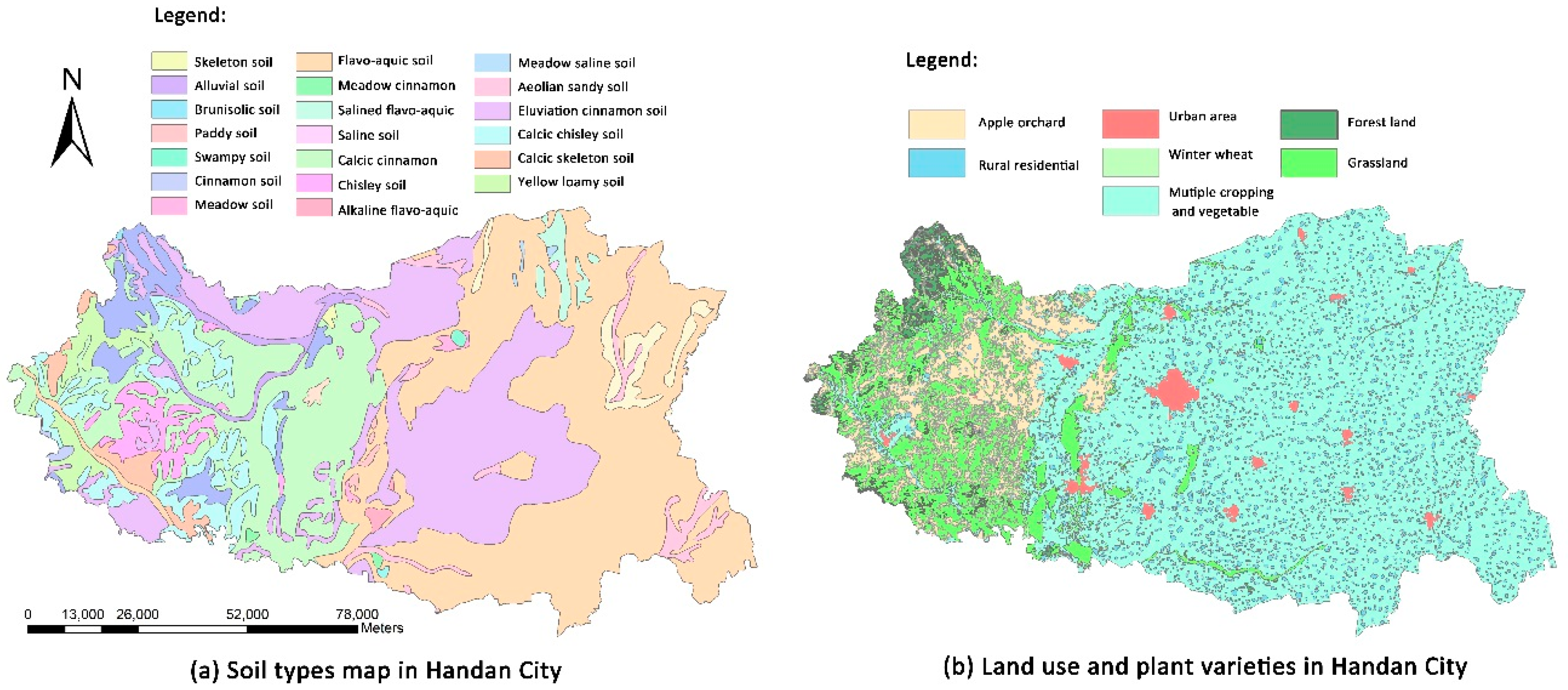
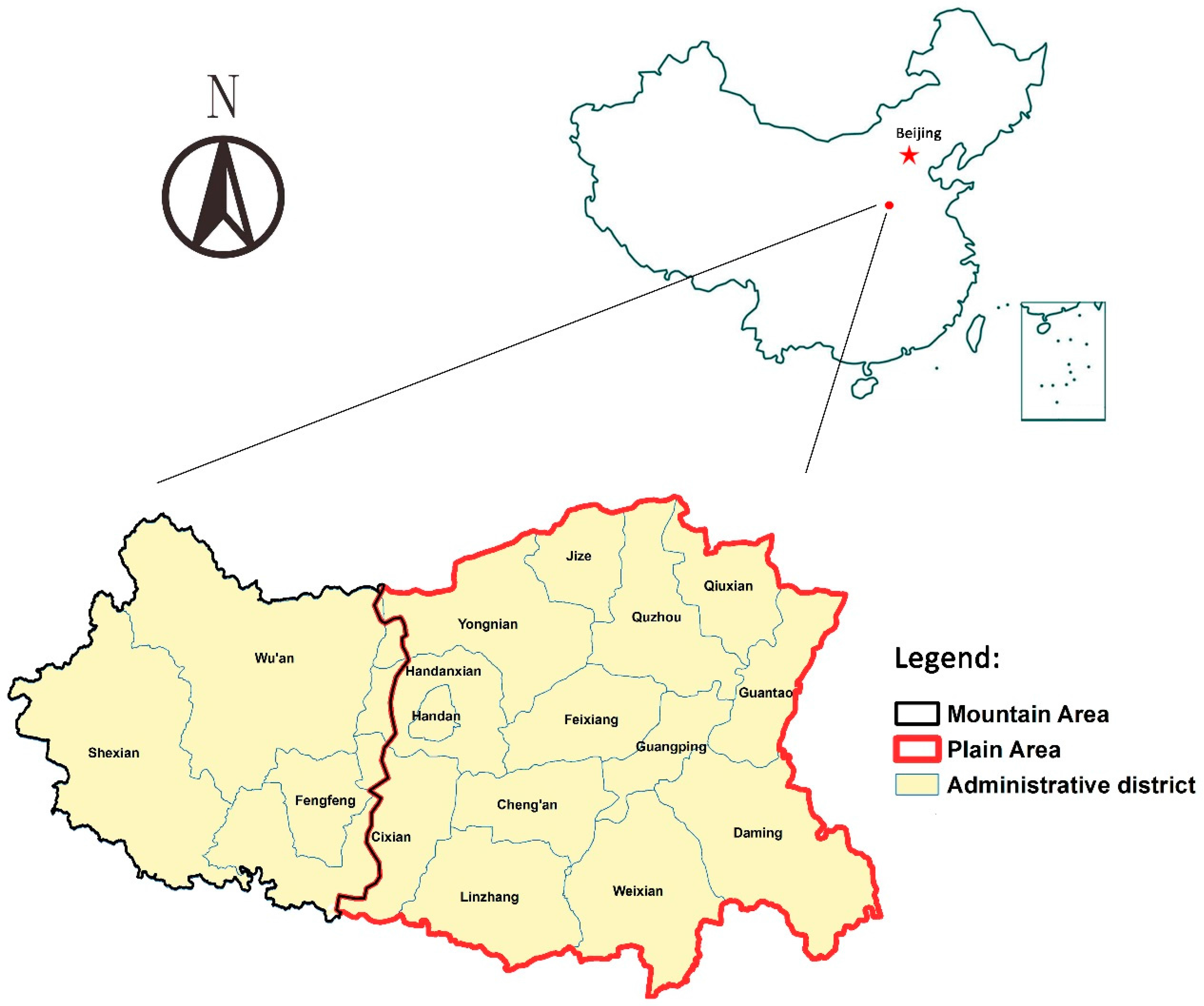
2.3. Overview of the Study Area

Handan City is located in the southern part of the North China Plain at latitude 36.07° N to 37.02° N and longitude 113.47° E to 115.47° E, which covers an area of 12,047 km2 (Figure 2). Handan City has a semi-arid continental monsoon climate with four distinct seasons and high spatially and temporally distributed precipitation. According to the statistics, the average annual precipitation is 548.9 mm, and the average annual temperature ranges from 12.5 °C to 14.2 °C. According to the local Water Resources Bulletin statistics, the water consumption from households and industries in Handan City increased dramatically from 2003 to 2012. During the last decade, household and industrial water consumption increased by 6.8% annually, reaching 5.3 × 10⁸ m3 in 2014 and accounting for 21.8% of the total water consumption in Handan City. Moreover, the average annual runoff water resources of Handan City have decreased dramatically from 5.8 × 10⁸ m3 (1956–2000 runoff data series) to 4.2 × 10⁸ m3 (2001–2010 runoff data series). Owing to the sharp increase in water consumption and the sharp decrease in runoff water resources, agricultural water has been diverted to other water sectors, which is a great threat to the sustainable development of agriculture and food security in this region.
Handan City has a long history of agricultural cultivation and is one of the most important grain and cotton production areas in the North China Plain. According to the Year Book of Agricultural Statistics, the annual grain production in Handan City was above 4.5 × 10⁹ kg from 2005 to 2012, ranking in the top three areas in Hebei Province. Winter wheat, cotton, and summer maize are the dominant crops. The average farmland area in this region in the past decade reached 660,000 ha, accounting for almost 10% of the total arable land in Hebei Province. For these reasons, Handan City was selected as the study area.
One of the most important objectives of this research is to simulate the soil moisture in the farmland. In MODCYCLE, the Green–Ampt method is used to simulate the soil water infiltration and percolation process using land use data, plant variety, and soil type as key parameters. In this research, the land use data in the study area were retrieved by remote sensing. Five main land use patterns are included in the study area: farmland, forest land, grassland, urban areas, and rural residential areas. Farmland covers the largest area of Handan City, accounting for 86% of the total area. The crop variety data in this research were collected from the Rural Statistical Yearbook of Hebei Province combined with the field survey. For the field survey, we visited more than 100 farmers to determine the crop varieties and planting areas, particularly in Daming and Quzhou County. The survey data were used to verify the reliability of the Rural Statistical Yearbook of Hebei Province. The statistics indicate nine crop varieties in the study area, with winter wheat, multiple cropping of wheat and summer maize, cotton, vegetables, and apple orchard as the five dominant crops. The soil-type data were collected from the China Soil Scientific Database and were validated through high-density sampling experiments. Generally, 22 soil types are included in the study region. The distribution maps of the planting varieties with land use and soil type in the study area are separately shown in Figure 3a,b.

3. Results

3.1. Model Construction

The input parameters required in the model construction process include basic geographic information, observed meteorological data, agricultural management regimes, and hydrological data. The basic geographic information includes topographical data, land use and crop varieties, soil type, and the main digital rivers and reservoirs in the study area, which are all used for delineation of the sub-basins and discretization of the HRUs. The observed meteorological data include precipitation, temperature, wind speed, radiation, and relative humidity at a daily timescale. The agricultural management regimes are important in the model because they depict the planting configuration and irrigation scheduling in the farmland. The hydrological data include river runoff, inflow and outflow of the reservoirs, and the observed soil moisture, which can be used for model calibration and validation. For convenience, only the observed soil moisture data were used for the initial calibration of the model. The data required for MODCYCLE are shown in Table 3.
In this study, the period of the simulation was 1998–2014. A warm-up period from 1996 to 1997 was also used for this model. All of the data were collected within this period. The data from 1998 to 2000 were used for model calibration, and those from 2001 to 2003 were used for model validation. Model calibration is an important process for improving the simulation accuracy and precision. Ten parameters were selected as the most sensitive parameters. Because the MODCYCLE is a newly developed model, the auto calibration module is not yet embedded. Therefore, we adopted the manual parameter adjustment method for parameter calibration. After more than 20 attempts and simulations, the optimal set of parameters were determined and selected, as shown in Table 4.

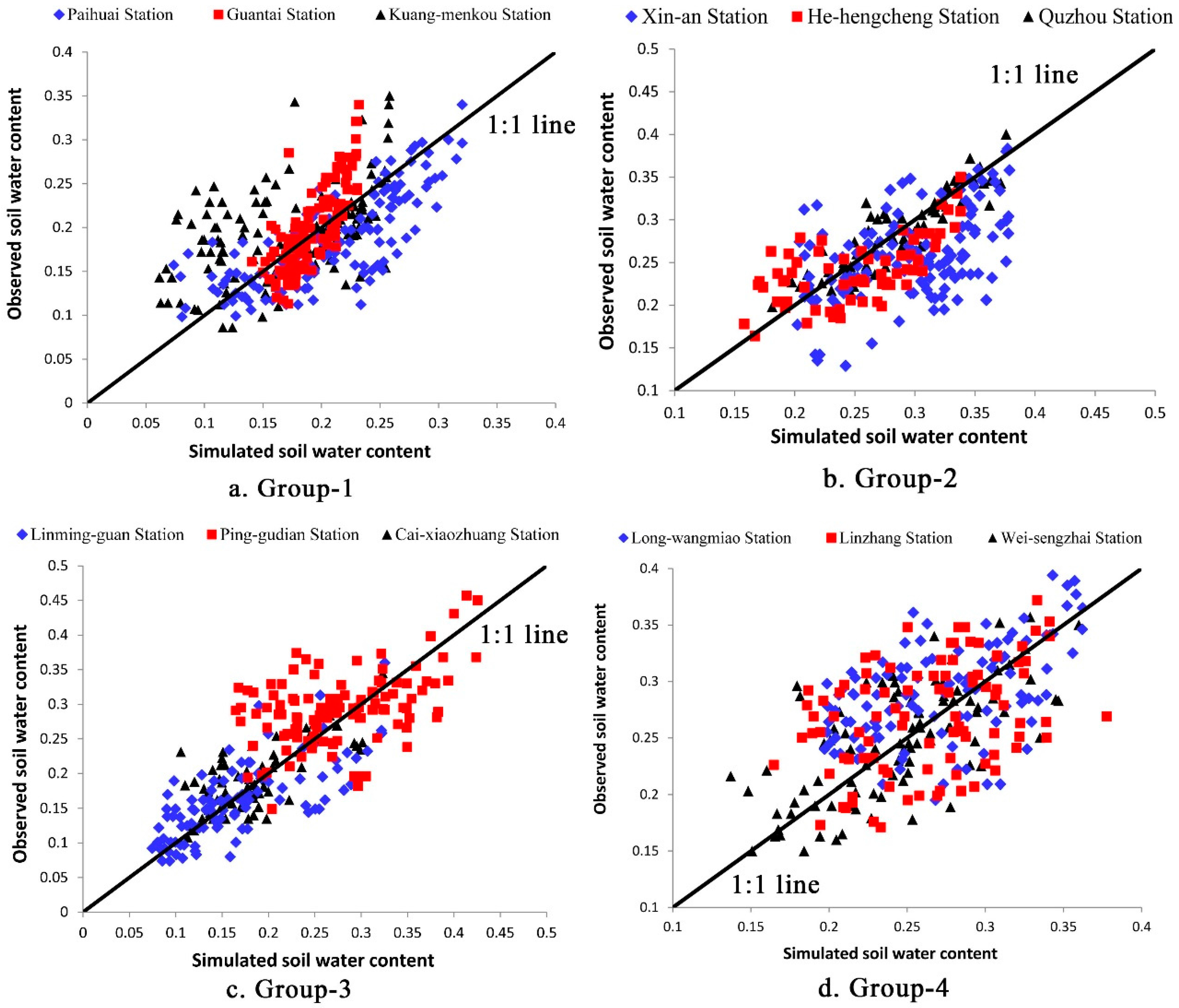
3.2. Model Validation

In our study, we compared the simulated and soil observed water contents to validate the model. The observed soil water content data were obtained by sampling in the soil profile, where the average depth of the soil profile was usually 600 mm. Four sampling points were selected in one soil profile at depths of 0–15 mm, 15–30 mm, 30–45 mm, and 45–60 mm. After the soil samples were collected, the soil water content was measured using the oven drying method. Based on the above measurements, the average soil water content in the entire soil profile was calculated as the weighted average value of the soil water content of the four sampling points. We collected the in situ observed soil moisture data from 12 soil moisture monitoring stations evenly distributed in the study area. A list of these stations is given in Table 5. For convenience, the 12 monitoring stations were also classified into four groups.
For validation, the simulated soil water content results in the HRUs in which the soil moisture monitoring stations are located were selected for comparison with the observed soil water content from the 12 monitoring stations. The depth of the soil water content simulated in MODCYCLE was as much as 3000 mm. However, to keep the depth of the simulation results consistent with the observed results, we extracted only the simulated soil water content of the shallow soil layer (0–60 mm) to make comparisons with the observed soil moisture data. According to the simulation and observed results, comparison charts were drawn separately for the four groups of soil moisture monitoring stations, as shown in Figure 4.
As shown in Figure 4, the points in which the x- and y-coordinates represent the simulated and observed values, respectively, were essentially distributed along the 1:1 lines. This demonstrates an obvious consistency between the simulated and observed results. To further illustrate and validate the simulation results, the relative error ( ER ) and correlation coefficient ( R ) were introduced to quantitatively depict the consistency between the simulated and the measured results. As shown in Table 6, the statistical results show good agreement between the simulated and observed soil water contents as well.
As shown in the table, the relative errors ( ER ) were all below 10%, and the correlation coefficients ( R ) were all above 0.7 except for the data of Long-wangmiao and Linzhang stations. Because these two stations are located in the east and south plain area of Handan City, where the anthropogenic influence on farmland hydrological process is stronger than that in other areas, the simulation accuracy is poorer compared with other stations. This problem is also a global concern in hydrology. Generally, the simulation results were convincible and acceptable. Therefore, it is feasible to use MODCYCLE for soil water availability evaluation in the study area.

3.3. Soil Water Availability Quantitatively Evaluation

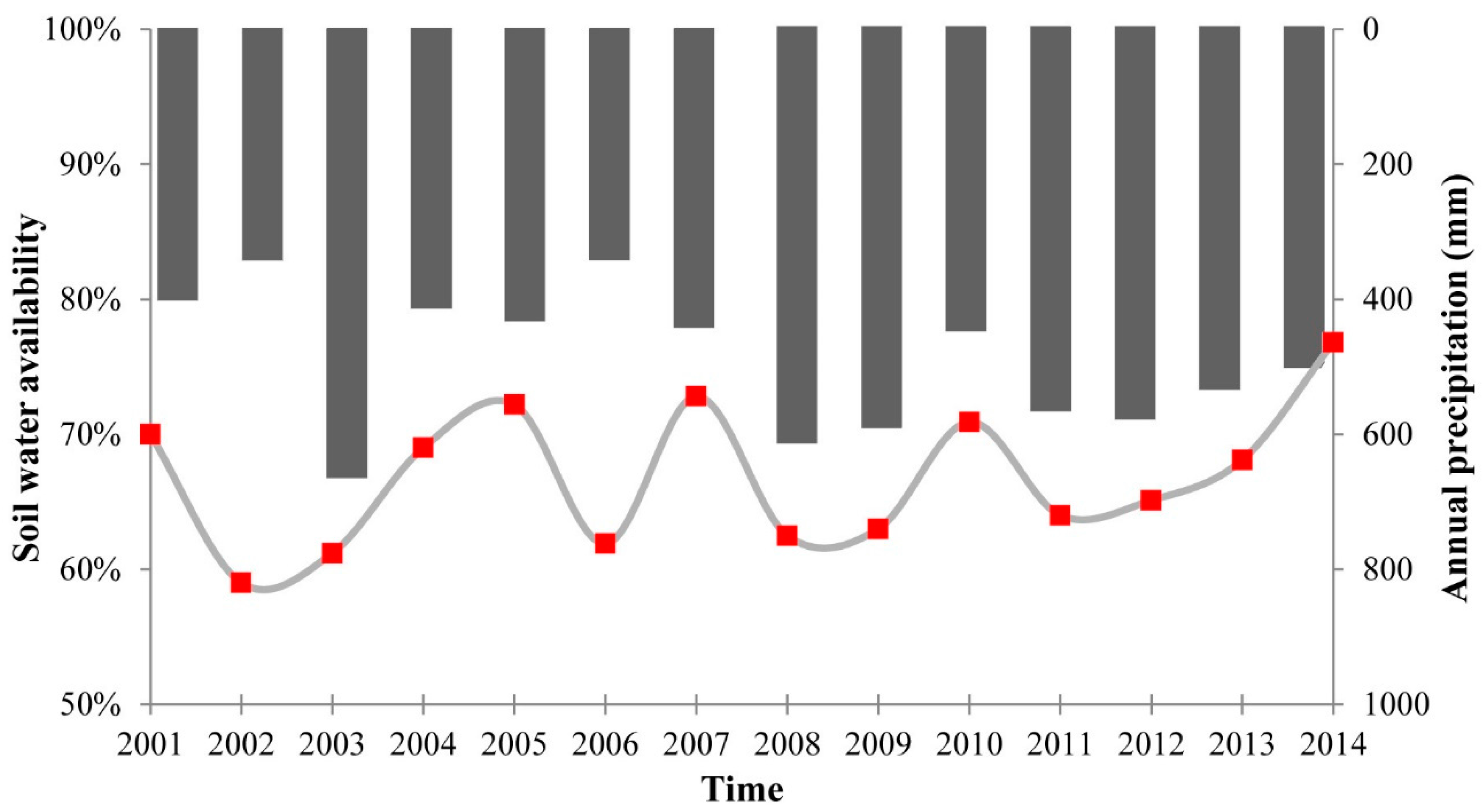
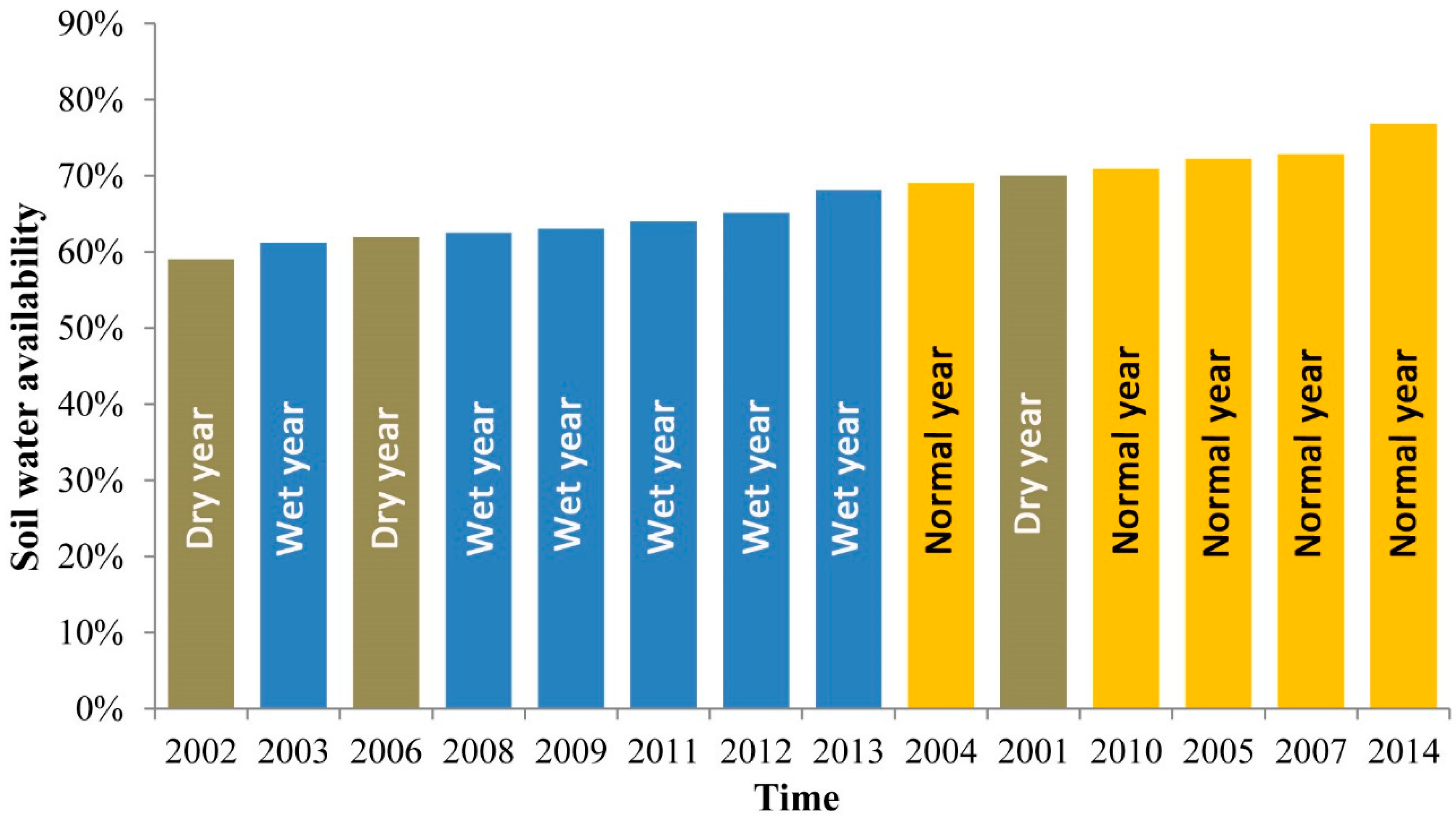
3.3.1. Temporal Perspective

As previously mentioned, the simulation period in this study was from 2001 to 2014. Based on the simulation results, the comprehensive soil water availability in the entire study area from 2001 to 2014 was calculated, as shown in Figure 5.
Figure 5 shows that the comprehensive SWA ranged from 59% to 76.8% in different years. The maximum value of 76.8% occurred in 2014 with yearly precipitation of 507 mm, and the minimum value of 59% occurred in 2002 with yearly precipitation of 346 mm. To analyse the relationship between soil water availability and the yearly precipitation of different hydrological level years, we ranked the SWA from 2001 to 2014 in ascending order. In addition, we determined the hydrological level of the different years according to the frequency analysis of precipitation. The resultant SWA ranking chart is shown in Figure 6.
Figure 6 shows the SWA from 2001 to 2014 sorted in ascending order. The high-soil-water-availability years were concentrated mainly in normal hydrological years. Five normal hydrological years were indicated in the simulation period, in which the SWA, shown by yellow bars in the figure, was much higher than that in dry and wet years, shown by brown and blue bars, respectively. Preliminary analysis indicated that in dry years, the water supply from precipitation was deficient, which cannot satisfy plant water requirements during the growing period. Therefore, the poor degree of matching between the soil water supply and plant water demand is the primary reason for the low SWA in dry years. In wet years, the precipitation was concentrated mostly in summer. Therefore, the available soil water distribution was extremely uneven, which in turn resulted in significant water loss in the rainy season, leaving plants vulnerable to drought in the sowing season.

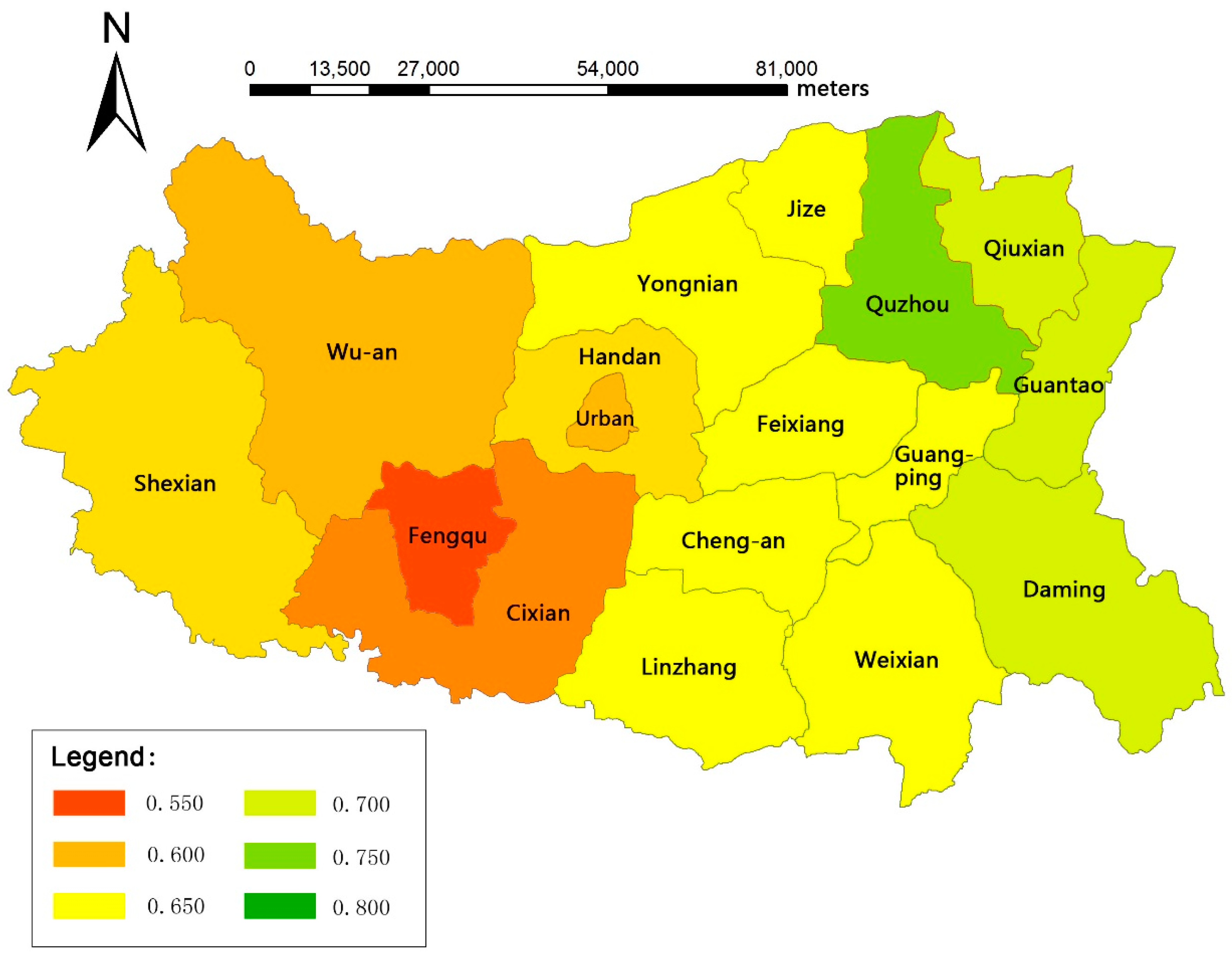
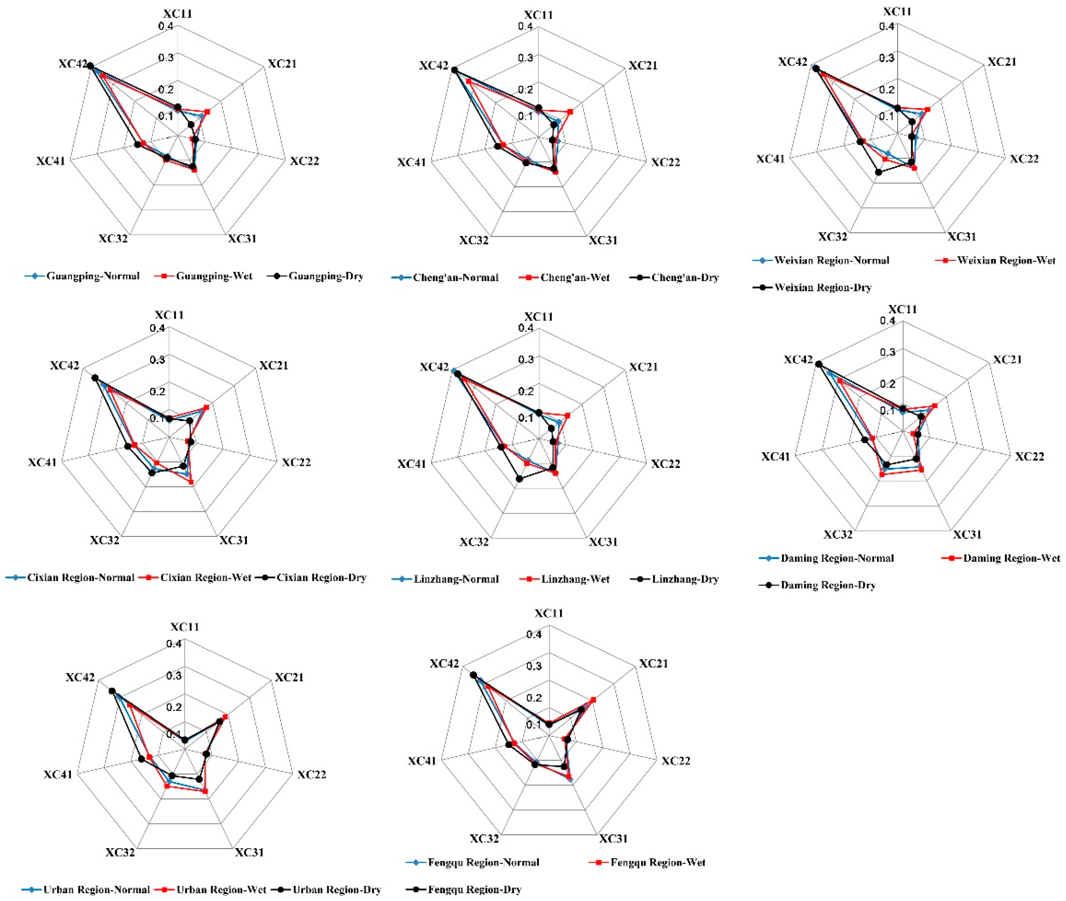
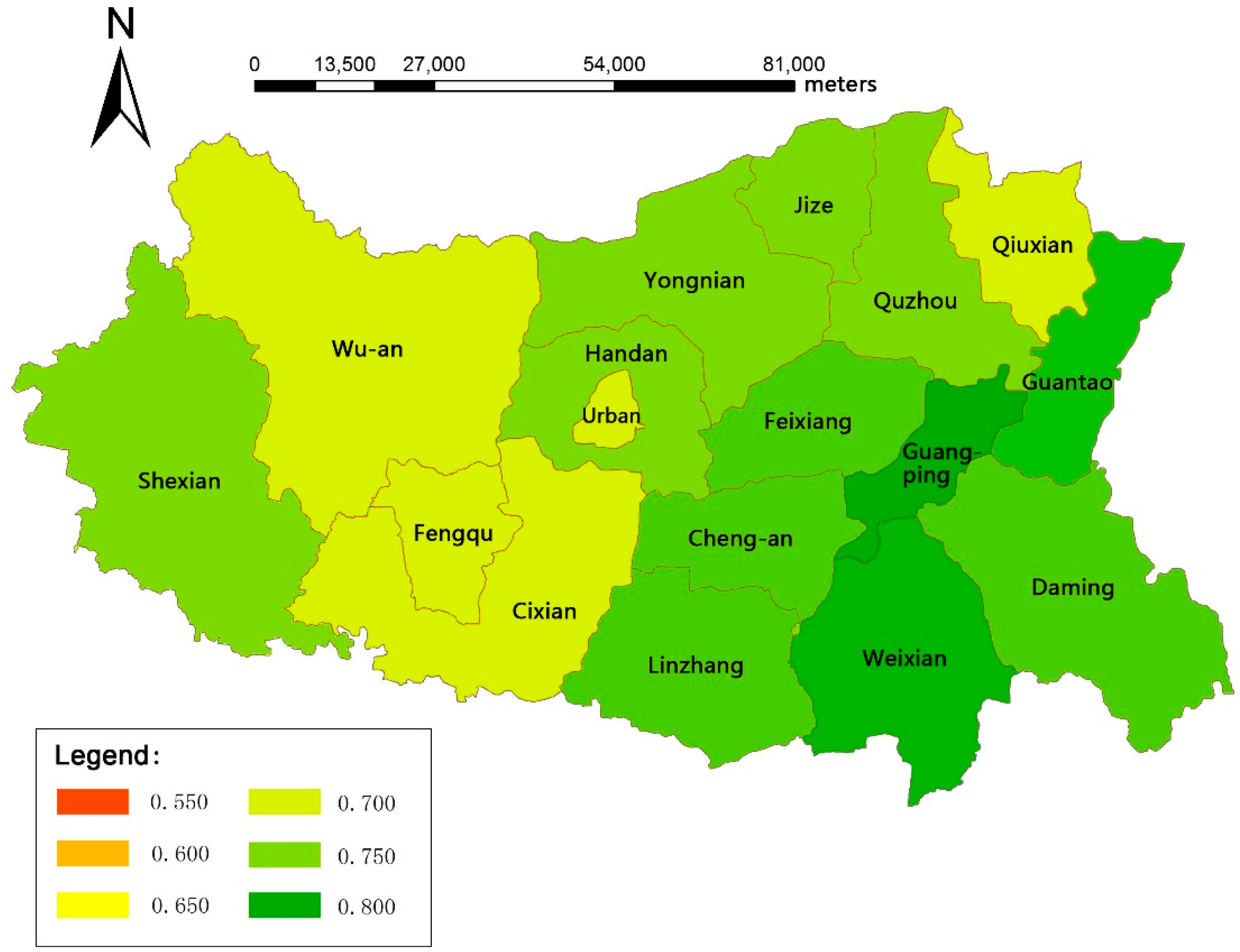
3.3.2. Spatial Perspective

The spatial distribution of the comprehensive SWA was mapped based on the simulation results. As the first step, the original values of the second-class indices were quantitatively calculated on the basis of Equation (3) to Equation (13). In this study, three different typical hydrological-level years were selected (e.g., a wet year, normal year, and dry year) through the frequency analysis of precipitation. The years 2006, 2010, and 2012 were determined to be typical dry, normal, and wet years. As the second step, the original values of the second-class indices were transformed to the standard values as shown in Table 7, Table 8 and Table 9 according to Equations (14) and (15). As the final step, the comprehensive SWA in different administrative regions was calculated on the basis of Equation (16).
As shown in Table 7, Table 8 and Table 9, because the index C11 represents the valid capacity of the soil reservoir, which is largely determined by the soil properties in the root zone, the standard values of the index in the three different hydrological years are the same. Spatial distribution maps of SWA in normal, wet, and dry years, based on the standard values of the second-class indexes, are shown in Figure 7, Figure 8 and Figure 9, respectively.
According to Table 7, Table 8 and Table 9 and Figure 7, Figure 8 and Figure 9, the average SWA of Handan City is 0.712, 0.649, and 0.619 in the hydrological normal, wet, and dry years, respectively. In general, when the SWA is below 0.7, the farmland soil water use efficiency (SWUE) is too low to be acceptable; when the SWA is above 0.8, the SWUE can be regarded as satisfactory. With this guidance, the average SWA of Handan City in the wet and dry years is not acceptable. Although the SWA in the normal year is higher than in the wet and dry years, there is still great potential for improvement. From a spatial distribution perspective, the SWA in the west and north mountainous area is lower than that in the east and south plain areas. This may be attributed to the following reasons. (1) The total precipitation in the south and east areas is higher than that in the north and west mountainous areas, and the annual temporal distribution of precipitation in the south and east areas is relatively even, which will increase the degree of matching between the soil water supply and crop water demand and will therefore improve the SWA in the south and east areas; (2) The root zone depth in the west and north mountainous area is thin. Therefore, the factor of the soil water storage capacity is smaller than that of the east and south plain areas; (3) Because the quality of arable land in the eastern and southern plain areas is better than that in the mountainous areas, multiple agricultural management measures such as irrigation and cultivation are implemented in the plain areas, which will improve the use efficiency of the agricultural water resources in the farmland.
Overall, the maps show that the variation in the SWA in different regions of the study area is large and that there is still great potential for improvement in the SWA and SWUE. The SWA distribution maps provide a visual display of its spatial and temporal distribution, allowing easy detection of the problematic regions for targeting specific measures for soil water regulation.

4. Discussion

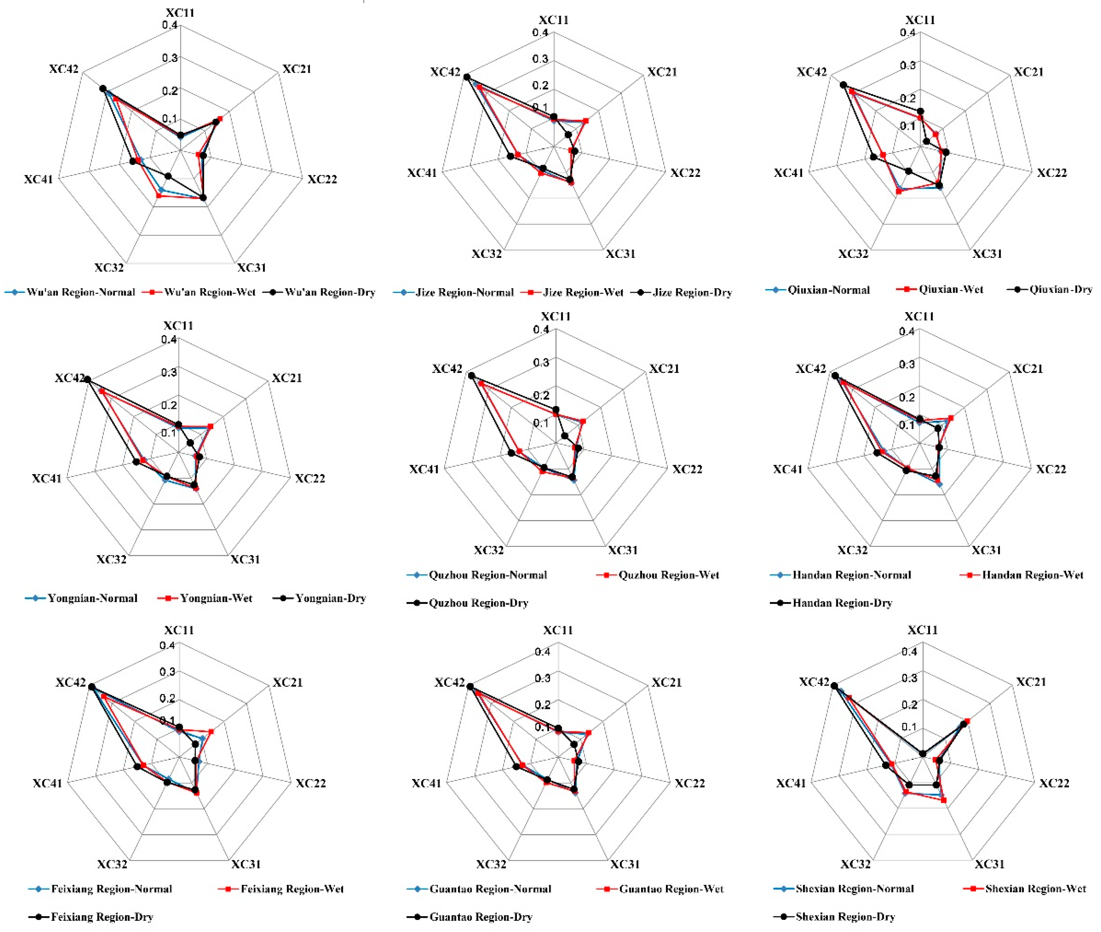
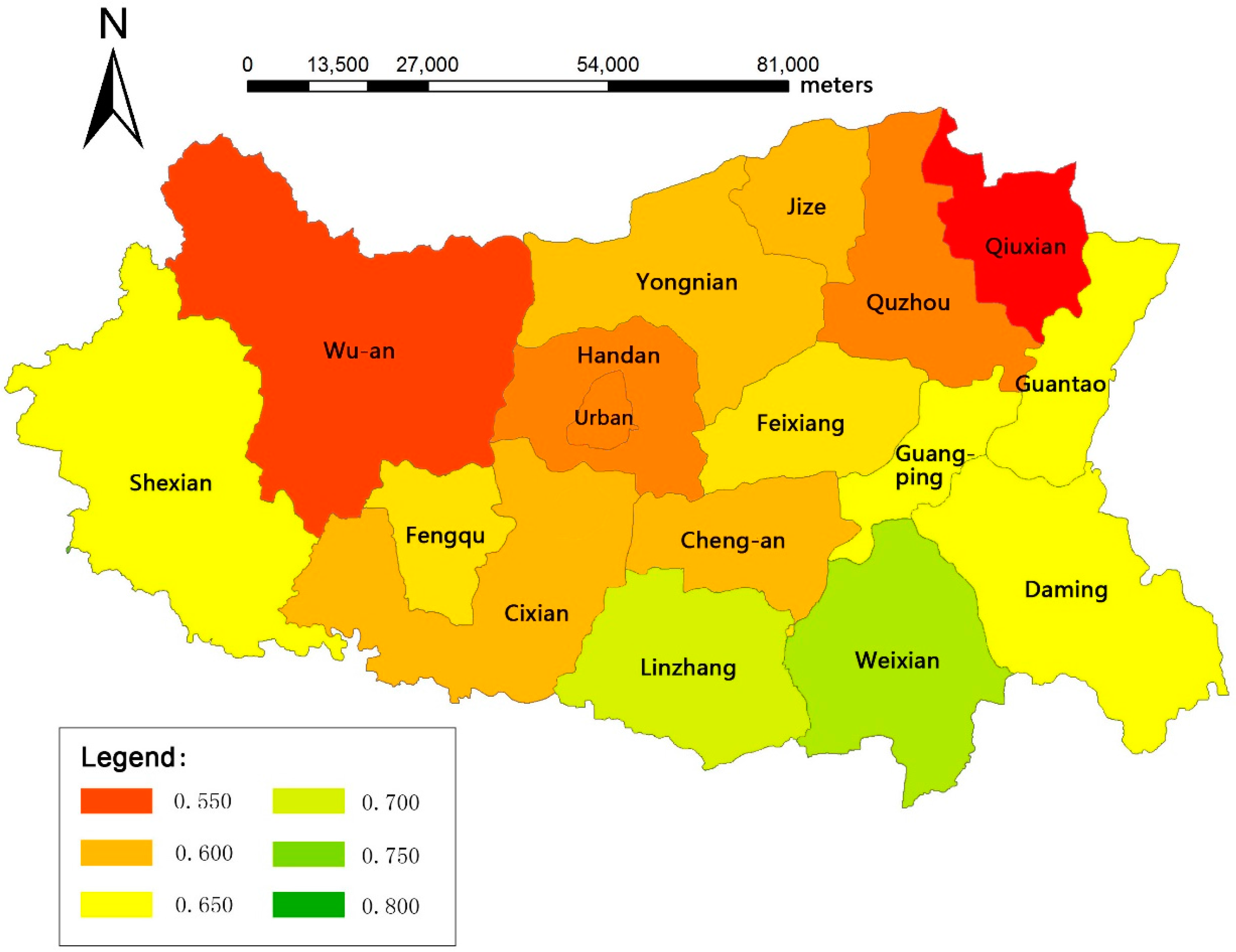
4.1. Analysis of the Main Factors Influencing the Soil Water Availability for Different Regions

As shown in Figure 7, Figure 8 and Figure 9, the SWA varies greatly in different regions because the values of the influencing factors ( C 11 , C 21 , C 22 , C 31 , C 32 , C 41 , and C 42 ) differ among regions. To analyze the main factors influencing the SWA for each region, we separately calculated the contribution ratio of each factor to the SWA in each region, and we plotted the statistical radar maps as shown in Figure 10 and Figure 11.
According to the radar maps, the contribution rate of different factors to the SWA in different regions can be clearly illustrated. Among the seven main factors, C42 is the most important with a contribution rate above 0.3 except for Wu’an, Cixian, and urban regions. The factors C21, C31, and C41 are also important with contribution rates between 0.1 and 0.2. Comparatively, C11, C22, and C32 contribute less to the total SWA with contribution rates around or below 0.1. According to the above analysis, to improve the total SWA, we should focus on the four factors (C42, C21, C31, and C41) and take measures to target increases in the contribution rates of these four factors. To analyse the potential for improvement in these contribution rates, we defined an index K to indicate the difference between the current value of the factor and the desired value of the factor, as shown in Equation (17):
  K n = ( V d V c ) / V d · 100 %
where K n is the potential of the factor n to be improved to a higher contribution rate to SWA, and V d is the maximum value of the contribution rate of the factor n , which is determined on the basis of Equation (16). The coefficient of each factor in Equation (16) can be regarded as the maximum value of the contribution rate of the corresponding factor; V c is the current value of the contribution rate of the factor n .
The potential of each factor in normal hydrological years for different regions was calculated on the basis of Equation (17), as shown in Table 10.
According to the analysis in Table 10, it is concluded that the potential for improvement of the factors differs among regions. For example, in the Wu’an Region, the indices K C 11 and K C 42 were much higher those of other factors, which means that the factors C 11 and C 42 have a large potential to be increased for a higher contribution to SWA. However, in the Jize Region, the indices K C 32 and K C 42 were much higher than those of other factors, which means that the factors C 32 and C 42 have large potential to be increased for a higher contribution to SWA. The values of the index K changed dramatically among the regions. Therefore, to improve the SWA in the study area, different measures must be taken according to the different potential of the factors in different regions.

4.2. Strategies to Improve Soil Water Availability

The concept of SWA is a new comprehensive indicator to quantitatively characterise the SWUE of farmland at a regional scale. This indicator not only considers the traditional index of field water use efficiency but also considers the soil water storage capacity of the soil layer, the actual capacity of the soil reservoir, and the spatial and temporal matching degree between the soil water supply and crop water demand. Therefore, SWA is a better index for SWUE evaluation and soil water management.
According to the analysis in Table 10, to improve the SWA, it is necessary to take different measures in different regions because the potential of the factors to be improved for a higher contribution to SWA is different.
First, in the Wu’an, Shexian, Cixian, Handan, and Fengqu regions, the factor C11 has a large potential for improvement because the index K is above 40% in the five regions and is as high as 90% in the Shexian Region. Therefore, using agronomic measures such as deep ploughing and straw returning to increase the valid capacity of the soil layer in the five regions is a key step for improving the SWA.
Second, in the Jize, Quzhou, Handan, Feixiang, Guantao, Guangping, Cheng’an, Weixian, and Linzhang regions, the factor C32 has a large potential for improvement because the index K is above 40% in the nine regions. This indicates that the degree of spatial matching between the soil water supply and crop water demand is very poor in the nine regions. Therefore, the planting structure in these regions should be adjusted to reduce the area of water-consuming crops such as winter wheat or to enlarge the area of water-efficient crops such as summer maize and potatoes.
Finally, as shown in Table 10, K C 42 was mostly above 30% in all 17 regions, although the index was only 29.6% in the Linzhang Region. Obviously, the potential of improving the C 42 factor is quite large in all of the regions in the entire study area. Therefore, increasing the soil water use efficiency for crop growth, such as mulching to reduce invalid evaporation and adopting regulated deficit irrigation, is a key approach for increasing the SWA.

5. Conclusions

Under the joint effects of climate change and human activities, the availability of blue water resources is severely reduced for agricultural production, particularly in arid and semi-arid areas. Therefore, soil water, known as green water resources, is becoming more and more important for sustainable development in agriculture and ecology. In this context, to improve the SWUE, this study put forward a new method to quantitatively evaluate the SWA based on a self-developed hydrological model at the regional scale and presented related strategies according to the main factors leading to low efficiency of soil water utilization. In summary, the main innovations in this research include two aspects. Firstly, this study originally proposed the concept of SWA and established a new evaluation index system to quantitatively calculate the SWA through the analytic hierarchy process method. Secondly, a self-developed distributed hydrological model (MODCYCLE) was introduced to simulate the soil moisture change process for SWA evaluation. However, modelling farmland soil moisture through a hydrological model is still challenging because of the high variability of underlying surface conditions and intensive human management measures, particularly in the Chinese farming system. Therefore, this study attempted the novel development of MODCYCLE considering the complicated tilling practices and management schemes in the North China Plain. Different from the SWAT model, MODCYCLE includes a special agricultural management module to depict the complex hydrological processes of Chinese farmland. Therefore, the simulation accuracy is greatly improved by using MODECYCLE to evaluate the SWA in the study area with complicated tilling practices and strong anthropogenic influences.
To verify the SWA evaluation method and the MODCYCLE model, Handan City in North China Plain was selected as a case study. The results show that the MODCYCLE model is an efficient tool for simulating the farmland hydrological process in the study area. According to the comparison between the observed soil moisture and simulated soil moisture results, the relative errors are all below 10%, and the correlation coefficients are almost above 0.7 except for Long-wangmiao and Linzhang stations. The SWA evaluation results indicate that the average SWA in the entire area ranges from 0.62 to 0.71 in different hydrological level years, which demonstrates that the potential is large for SWA improvement for a higher SWUE. However, the soil water availability changes greatly in different regions because the main factors influencing the SWA are different. Based on these findings, we suggest that managers can use the SWA index system to identify the main factors causing low soil water utilization efficiency in different regions and to select and determine the strategies for improving the SWA. Improving the reliability of the hydrological model is the foundation for SWA evaluation. However, owing to the complicated tillage practices and irrigation schemes in China, the farmland hydrological characteristics vary extensively among different regions, which poses a great challenge for model calibration and validation. Therefore, more attention should be paid to model improvement and validation when the model is adapted to other regions in future studies.

Acknowledgments

The researchers thank the Chinese National Natural Science Foundation (No. 51409275, No. 51309246 and No. 71503265) for their support of this study. The study was also supported by Natural Science Basic Research Plan in Shaanxi Province of China (No. 2016JQ5076), the Open Research Fund of the State Key Laboratory of Simulation and Regulation of Water Cycle in River Basin at the China Institute of Water Resources and Hydropower Research (IWHR-SKL-201601) and the Ph.D. Start-up Fund of Northwest A&F University (2452015344). The help provided by Wenxiang Pan, Miao Sun, and Qi Zhao is also appreciated.

Author Contributions

Xuerui Gao established the soil water availability evaluation system and constructed the MODCYCLE model. Jianhua Wang proposed the concept of soil water availability and designed the preliminary road map for this study. Pute Wu and Yong Zhao analysed the data and validated the model. Xining Zhao and Fan He revised the first draft.

Conflicts of Interest

The authors declare no conflict of interest.

References

  1. Xu, X.; Yang, D.; Yang, H.; Lei, H. Attribution analysis based on the Budyko hypothesis for detecting the dominant cause of runoff decline in Haihe basin. J. Hydrol. 2014, 510, 530–540. [Google Scholar] [CrossRef]
  2. Lema, M.A.; Majule, A.E. Impacts of climate change, variability and adaptation countermeasures on agriculture in semiarid areas of Tanzania: The case of Manyoni District in Singida Region, Tanzania. Afr. J. Environ. Sci. Technol. 2009, 3, 206–218. [Google Scholar]
  3. Robinson, D.A.; Campbell, C.S.; Hopmans, J.W.; Hornbuckle, B.K.; Jones, S.B.; Knight, R.; Ogden, F.; Selker, J.; Wendroth, O. Soil moisture measurements for ecological and hydrological watershed scale observatories: A review. Vadose Zone J. 2008, 7, 358–389. [Google Scholar] [CrossRef]
  4. Walker, J.P.; Houser, P.R.; Willgoose, G.R. Active microwave remote sensing for soil moisture measurement: A field evaluation using ERS-2. Hydrol. Process. 2004, 18, 1975–1997. [Google Scholar] [CrossRef]
  5. Deans, J.D.; Milne, R. An electrical recording soil moisture tensiometer. Plant Soil 1978, 50, 509–513. [Google Scholar] [CrossRef]
  6. Kodikara, J.; Rajeev, P.; Chan, D.; Gallage, C. Soil moisture monitoring at the field scale using neutron probe. Can. Geotech. J. 2014, 51, 332–345. [Google Scholar] [CrossRef] [Green Version]
  7. Dasberg, S.; Dalton, F.N. Time domain reflectometry field measurements of soil water content and electrical conductivity. Soil Sci. Soc. Am. J. 1985, 49, 293–297. [Google Scholar] [CrossRef]
  8. Dirksen, C.; Dasberg, S. Improved calibration of time domain reflectometry soil water content measurements. Soil Sci. Soc. Am. J. 1993, 57, 660–667. [Google Scholar] [CrossRef]
  9. Tanaka, D.L.; Aase, J.K. Fallow method influences on soil water and precipitation storage efficiency. Soil Till. Res. 1987, 9, 307–316. [Google Scholar] [CrossRef]
  10. Zegelin, S.J.; White, I.; Jenkins, D.R. Improved field probes for soil water content and electrical conductivity measurement using time domain reflectometry. Water Resour. Res. 1989, 25, 2367–2376. [Google Scholar] [CrossRef]
  11. Gao, X.; Wu, P.; Zhao, X.; Wang, J.; Shi, Y.; Zhang, B.; Tian, L.; Li, H. Estimation of spatial soil moisture averages in a large gully of the Loess Plateau of China through statistical and modeling solutions. J. Hydrol. 2013, 486, 466–478. [Google Scholar] [CrossRef]
  12. Wagner, W.; Lemoine, G.; Rott, H. A Method for Estimating Soil Moisture from ERS Scatterometer and Soil Data. Remote Sens. Environ. 1999, 70, 191–207. [Google Scholar] [CrossRef]
  13. Schmugge, T.J.; Kustas, W.P.; Ritchie, J.C.; Jackson, T.J.; Rango, A. Remote sensing in hydrology. Adv. Water Resour. 2002, 25, 1367–1385. [Google Scholar] [CrossRef]
  14. Vereecken, H.; Huisman, J.A.; Bogena, H.; Vanderborght, J.; Vrugt, J.A.; Hopmans, J.W. On the value of soil moisture measurements in vadose zone hydrology: A review. Water Resour. Res. 2008, 44, W00D06. [Google Scholar] [CrossRef]
  15. Ulaby, F.T.; Dubois, P.C.; Van Zyl, J. Radar mapping of surface soil moisture. J. Hydrol. 1996, 184, 57–84. [Google Scholar] [CrossRef]
  16. Fernández-Prieto, D.; van Oevelen, P.; Su, Z. Advances in Earth observation for water cycle science. Hydrol. Earth Syst. Sci. 2012, 16, 543–549. [Google Scholar] [CrossRef]
  17. Kong, X.; Dorling, S.R. Near-surface soil moisture retrieval from ASAR Wide Swath imagery using a Principal Component Analysis. Int. J. Remote Sens. 2008, 29, 2925–2942. [Google Scholar] [CrossRef]
  18. Ford, T.W.; Harris, E.; Quiring, S.M. Estimating root zone soil moisture using near-surface observations from SMOS. Hydrol. Earth Syst. Sci. 2014, 18, 139–154. [Google Scholar] [CrossRef]
  19. Martínez-Fernández, J.; González-Zamora, A.; Sánchez, N.; Gumuzzio, A.; Herrero-Jiménez, C.M. Satellite soil moisture for agricultural drought monitoring: Assessment of the SMOS derived Soil Water Deficit Index. Remote Sens. Environ. 2016, 177, 277–286. [Google Scholar] [CrossRef]
  20. Ni-Meister, W. Recent advances on soil moisture data assimilation. Phys. Geogr. 2008, 29, 19–37. [Google Scholar] [CrossRef]
  21. Montaldo, N.; Albertson, J.D. Multi-scale assimilation of surface soil moisture data for robust root zone moisture predictions. Adv. Water Resour. 2003, 26, 33–44. [Google Scholar] [CrossRef]
  22. Reichle, R.H.; Koster, R.D. Global assimilation of satellite surface soil moisture retrievals into the NASA Catchment land surface model. Geophys. Res. Lett. 2005, 32, 177–202. [Google Scholar]
  23. Kim, S. Time series modeling of soil moisture dynamics on a steep mountainous hillside. J. Hydrol. 2016, 536, 37–49. [Google Scholar] [CrossRef]
  24. Gao, X.; Lu, C.; Luan, Q.; Zhang, S.; Liu, J.; Han, D. Mapping farmland-soil moisture at a regional scale using a distributed hydrological model: Case study in the north china plain. J. Irrig. Drain. Eng. 2016, 142, 04016029. [Google Scholar] [CrossRef]
  25. Fu, B.; Yang, Z.; Wang, Y.; Zhang, P. A mathematical model of soil moisture spatial distribution on the hill slopes of the Loess Plateau. Sci. China Earth Sci. 2001, 44, 395–402. [Google Scholar] [CrossRef]
  26. Zhang, J.E.; Lu, C.Y.; Qin, D.Y.; Guo, Y.X.; Ge, H.F. Regional runoff study based on MODCYCLE distributed hydrology model. Trans. Chin. Soc. Agric. Eng. 2011, 27, 65–71. [Google Scholar]
  27. Arnold, J.G.; Allen, P.M.; Bernhardt, G. A comprehensive surface-ground water flow model. J. Hydrol. 1993, 142, 47–69. [Google Scholar] [CrossRef]
  28. Mapfumo, E.; Chanasyk, D.S.; Willms, W.D. Simulating daily soil water under foothills fescue grazing with the soil and water assessment tool model (Alberta, Canada). Hydrol. Process. 2004, 18, 2787–2800. [Google Scholar] [CrossRef]
  29. Li, M.X.; Ma, Z.G.; Du, J.W. Regional soil moisture simulation for Shaanxi Province using SWAT model validation and trend analysis. Sci. China Earth Sci. 2010, 53, 575–590. [Google Scholar] [CrossRef]
  30. Zhang, J.E.; Lu, C.Y.; Qin, D.Y.; Wang, R.D. MODCYCLE—An object oriented modularized hydrological model II. Application. Shuilixuebao. J. Hydraul. Eng. 2012, 43, 1287–1295. [Google Scholar]
  31. Liu, J.; Wei, C.; Xie, Q.; Zhang, W. Capacities of soil water reservoirs and their better regression models by combining “merged groups PCA” in Chongqing, China. Acta Ecol. Sin. 2014, 34, 53–65. [Google Scholar] [CrossRef]
  32. Gu, S.X.; Xiong, Y.L.; Xu, X.; Wei, C.F.; Liu, G.C. Research progress on soil reservoir and utilization rainfall resources. Southwest China J. Agric. Sci. 2003, 16, 29–32. [Google Scholar]
  33. Zhang, J.; Lu, C.; Qin, D.; Liu., M. Regional “four-water” transformation based on distributed hydrological model. Adv. Water Sci. 2011, 22, 595–604. [Google Scholar]
  34. Stanhill, G. Water use efficiency. Adv. Agron. 1986, 39, 53–85. [Google Scholar]
  35. Saaty, T.L. A scaling method for priorities in hierarchical structures. J. Math. Psychol. 1977, 15, 234–281. [Google Scholar] [CrossRef]
  36. Vaidya, O.S.; Kumar, S. Analytic hierarchy process: An overview of applications. Eur. J. Oper. Res. 2006, 169, 1–29. [Google Scholar] [CrossRef]
  37. Saaty, T.L. The modern science of multicriteria decision making and its practical applications: The AHP/ANP approach. Oper. Res. 2013, 61, 1101–1118. [Google Scholar] [CrossRef]
  38. Sara, J.; Stikkelman, R.M.; Herder, P.M. Assessing relative importance and mutual influence of barriers for CCS deployment of the ROAD project using AHP and DEMATEL methods. Int. J. Greenh. Gas Control 2015, 41, 336–357. [Google Scholar] [CrossRef]
  39. Wind, Y.; Saaty, T.L. Marketing applications of the analytic hierarchy process. Manag. Sci. 1980, 26, 641–658. [Google Scholar] [CrossRef]
  40. Saaty, T.L. Decision making-the analytic hierarchy and network processes (AHP/ANP). J. Syst. Sci. Syst. Eng. 2004, 13, 1–35. [Google Scholar] [CrossRef]
  41. The Ministry of Economy, Trade, and Industry (METI) of Japan; The United States National Aeronautics and Space Administration (NASA). ASTER Global Digital Elevation Model (GDEM). Available online: http://www.jspacesystems.or.jp/ersdac/GDEM/E/4.html (accessed on 12 October 2015).
  42. National Meteorological Information Centre of China. China Meteorological Data Network. Available online: http://data.cma.cn/data/detail/dataCode/A.0012.0001.html (accessed on 18 February 2016).
Figure 1. Hydrological processes in the 1D soil column method.
Water 08 00360 g001
Figure 2. Location map of the study area.
Water 08 00360 g002
Figure 3. Distribution of soil and land use in Handan City.
Water 08 00360 g003
Figure 4. Comparison of observed values and simulated values of the 12 monitoring stations.
Water 08 00360 g004
Figure 5. Comprehensive soil water availability in the simulation period.
Water 08 00360 g005
Figure 6. SWA ranking in different hydrological level years.
Water 08 00360 g006
Figure 7. Spatial distribution of SWA in the normal hydrological year (2010).
Water 08 00360 g007
Figure 8. Spatial distribution of SWA in the hydrological wet year (2012).
Water 08 00360 g008
Figure 9. Spatial distribution of SWA in the hydrological dry year (2006).
Water 08 00360 g009
Figure 10. Contribution ratio of different factors to the comprehensive SWA in Wu’an, Jize, Qiuxian, Yongnian, Quzhou, Handan, Feixiang, Guantao, and Shexian regions in different hydrological-level years. As shown in Table 1, the factor of C11 represents the valid physical capacity of the soil reservoir, C21 represents the average value of the annual empty storage capacity of the soil reservoir, C22 is the factor for the average annual variation of the empty storage capacity of the soil reservoir, C31 represents the factor for the temporal matching degree between the soil water supply and crop water demand, C32 represents the factor for the spatial matching degree between the soil water supply and crop water demand, C41 is the factor for the soil water conversion efficiency, and C42 is the factor for the crop use efficiency of the soil water.
Water 08 00360 g010
Figure 11. Contribution ratio of different factors to the comprehensive SWA in Guangping, Cheng’an, Weixian, Cixian, Linzhang, Daming, Fengqu, and urban regions in different hydrological-level years. As shown in Table 1, the factor of C11 represents the valid physical capacity of the soil reservoir, C21 represents the average value of the annual empty storage capacity of the soil reservoir, C22 is the factor for the average annual variation of the empty storage capacity of the soil reservoir, C31 represents the factor for the temporal matching degree between the soil water supply and crop water demand, C32 represents the factor for the spatial matching degree between the soil water supply and crop water demand, C41 is the factor for the soil water conversion efficiency, and C42 is the factor for the crop use efficiency of the soil water.
Water 08 00360 g011
Table 1. Evaluation index system for farmland soil water availability.
FactorFirst-Class IndexSecond-Class IndexDescription
Availability of soil water quantityThe soil water storage capacity (C1)The valid capacity of soil reservoir (C11)The valid water supply capacity (equivalent water depth) of the soil in the crop root zone, mm.
Operational characteristics of farmland soil reservoir (C2)Average value of annual empty storage capacity of the soil reservoir (C21)To characterise the average soil water shortage severity in the soil root zone within a year, mm.
Average annual variation of empty storage capacity of the soil reservoir (C22)To characterise the fluctuation of water shortage severity in the root zone within a year, dimensionless.
The spatial and temporal matching of soil water resource between supply and demandTemporal and spatial matching degree (C3)Temporal matching degree index (C31)The temporal matching degree between soil water supply and crop water requirement, dimensionless.
Spatial matching degree index (C32)The spatial matching degree between soil water supply and crop water requirement, dimensionless.
The efficiency of soil water transformation and plant uptakeSoil water transformation and crop absorption efficiency (C4)Soil water conversion efficiency (C41)To characterise the efficiency of water transforming from other types to soil water, dimensionless.
Crop absorption efficiency (C42)To characterise the efficiency the soil water is absorbed by crops and plants, dimensionless.
Table 2. Pair-wise comparison matrix of the factors (C1, C2, C3, and C4).
Factors C 1 C 2 C 3 C 4
C 1 10.250.50.125
C 2 410.50.333
C 3 2210.5
C 4 8321
Table 3. Data required for MODCYCLE model construction.
Data TypesDetailSource
Basic geographic information1. DEM (90 m × 90 m)Land Processes Distributed Active Archive Center of USA [41].
2. Land use map (1:100,000)The map was retrieved by remote sensing data, which are provided by Data Center for Resources and Environmental Sciences, Chinese Academy of Sciences (RESDC): http://www.resdc.cn
3. Soil property map (1:100,000)China Soil Scientific Database: http://www.soil.csdb.cn/
4. Digital river and reservoir (1:250,000)The digital river and reservoir map was drawn based on the paper map using GIS tool
5. Groundwater aquifer dataThe data were collected from Handan Water Conservancy Bureau
Meteorological observed data1. Daily rainfallChina Meteorological Data Network [42].
2. Average daily temperature
3. Average daily wind speed
4. Daily sun radiation
5. Average relative humidity
Agricultural management regimes1. Crop varietiesThe data were collected from “Rural Statistical Yearbook of Hebei Province”
2. Planting configuration
3. Irrigation regimes
Hydrological data1. Runoff in 5 main riversThe data were collected from Handan Water Conservancy Bureau
2. Inflow and outflow in 12 reservoirs
3. Soil moisture data measured in 12 monitoring stations
Others1. socio-economic water consumption data.The data were derived from “Statistical Yearbook of Handan”
Table 4. Key parameters and their optimal values used in MODCYCLE.
NO.ParameterDescriptionOptimal Value
1MXSPMaximum water depth stored in the surface of farmland, which is closely related to runoff generation100 mm
2ESCOCorrection coefficient in calculating soil evaporation from the soil profile, which is an important factor affecting water volume evaporated in different soil layers0.70
3EPCOCorrection coefficient in calculating the plant evapotranspiration from the soil profile, which affects water volume absorbed by plant in different soil layers0.96
4FFCBThe ratio between initial soil moisture and field capacity of the soil profile0.6
5GWECCoefficient in calculating the water volume recharged from groundwater aquifer to soil profile0.89
6SLAGRunoff lag coefficient3.2
7SOLKThe hydraulic conductivity of different soil layers2–150 mm/h
8SOLADepth of available water in the soil profile100–600 mm
9CANMMaximum water depth intercepted by crop canopy6 mm
10BIOEThe radiation-use efficiency of the plant15–40 (kg/ha)/(MJ/m2)
Table 5. Soil moisture monitoring stations in the study area.
GroupIDStation NameCountyWater SourceLatitudeLongitude
Group-11Paihuai StationWu’anRain-fed114.0236.62
2Guantai StationCixianRain-fed114.0836.33
3Kuang-menkou StationShexianRain-fed113.7836.45
Group-24Xin-an StationFeixiangRain-fed114.6836.55
5He-hengcheng StationCheng’anRain-fed114.5736.48
6Quzhou StationQuzhouRain-fed114.9736.78
Group-37Linming-guan StationYongnianRain-fed114.4836.67
8Ping-gudian StationGuangpingRain-fed115.0736.57
9Cai-xiaozhuang StationWeixianIrrigation114.9336.28
Group-410Long-wangmiao StationDamingIrrigation115.2236.22
11Linzhang StationLinzhangIrrigation114.6236.35
12Wei-sengzhai StationGuantaoIrrigation115.3836.72
Table 6. Statistical results showing the consistency between observed and simulated values.
IDStation NameObserved Average ValueSimulated Average ValueER (%)R
1Paihuai Station0.1730.1898.830.87
2Guantai Station0.2010.1876.940.82
3Kuang-menkou Station0.1550.1521.790.95
4Xin-an Station0.2750.3019.330.76
5He-hengcheng Station0.2410.2534.750.72
6Quzhou Station0.2410.2534.750.75
7Linming-guan Station0.2480.2432.020.95
8Ping-gudian Station0.2610.2641.150.97
9Cai-xiaozhuang Station0.1950.1873.930.72
10Long-wangmiao Station0.3130.2897.450.6
11Linzhang Station0.2570.261.470.52
12Wei-sengzhai Station0.2480.2552.820.77
Table 7. Standard values of the second-class indices and the total SWA of different regions in the normal year (2010).
Normal Year (2010)XC11XC21XC22XC31XC32XC41XC42U
Wu’an Region0.4160.8360.8061.000.820.9150.5130.701
Jize Region0.8990.7300.7540.830.550.9000.6110.703
Qiuxian Region0.9830.3770.8640.930.960.9430.5250.701
Yongnian Region0.8480.7360.7100.830.630.8590.6060.701
Quzhou Region0.9810.6170.8360.830.560.9100.5790.688
Handan Region0.7230.6800.8390.950.580.9130.6250.714
Feixiang Region0.9140.5720.8400.830.510.9310.6890.718
Guantao Region0.8950.7090.8060.830.520.9170.6590.720
Shexian Region0.1000.9760.7230.940.900.8720.6980.764
Guangping Region0.9210.6290.8400.830.510.9220.6860.724
Cheng’an Region0.9190.4930.8440.830.530.9330.6850.710
Weixian Region0.8790.6290.8130.830.490.9320.6910.720
Cixian Region0.5730.7850.8000.830.710.8770.5110.667
Linzhang Region0.8930.5170.8420.830.530.9220.7040.717
Daming Region0.7710.7410.7340.941.000.9210.6680.786
Urban Region0.2810.8890.8710.950.750.8910.5290.692
Fengqu Region0.3550.8960.7021.000.610.8690.5410.680
Average in the whole area0.7270.6720.7980.870.660.9100.6230.712
Table 8. Standard values of the second-class indices and the total SWA of different regions in the wet year (2012).
Wet Year (2012)XC11XC21XC22XC31XC32XC41XC42U
Wu’an Region0.4160.7840.6080.890.840.8730.4140.628
Jize Region0.8990.7280.6840.770.570.8490.5510.665
Qiuxian Region0.9830.3580.8740.811.000.9210.5290.689
Yongnian Region0.8480.7290.7110.770.520.8390.5600.659
Quzhou Region0.9810.6410.7740.770.630.8940.5680.683
Handan Region0.7230.6860.7030.770.520.8650.5420.640
Feixiang Region0.9140.7270.6710.770.540.8570.5620.666
Guantao Region0.8950.7280.6630.770.570.8920.6180.694
Shexian Region0.1000.9750.4910.90.720.7080.5260.639
Guangping Region0.9210.7040.6010.770.550.8560.5810.668
Cheng’an Region0.9190.7370.6520.770.540.8660.5310.655
Weixian Region0.8790.7040.5430.770.570.8420.5660.657
Cixian Region0.5730.7570.660.870.50.7410.3940.574
Linzhang Region0.8930.6820.6730.770.550.8450.5720.663
Daming Region0.7710.7780.4350.891.000.7700.5010.685
Urban Region0.2810.8820.7650.870.760.8070.3920.613
Fengqu Region0.3550.8810.5340.770.530.7240.3960.558
Average in the whole area0.7270.7160.640.810.650.8380.5250.649
Table 9. Standard values of the second-class indices and the total SWA of different regions in the dry year (2006).
Dry Year (2006)XC11XC21XC22XC31XC32XC41XC42U
Wu’an Region0.4160.6590.7370.820.450.9240.4680.591
Jize Region0.8990.3020.7550.650.430.9400.5880.606
Qiuxian Region0.9830.1210.8610.710.450.9450.4840.564
Yongnian Region0.8480.2480.7760.650.480.9330.6290.619
Quzhou Region0.9810.1780.7910.650.470.9420.5560.590
Handan Region0.7230.3810.7180.650.540.9290.5730.608
Feixiang Region0.9140.3390.5810.650.500.9220.5990.613
Guantao Region0.8950.3380.7520.650.460.9370.6130.624
Shexian Region0.1000.9230.6580.60.600.8750.6500.658
Guangping Region0.9210.2980.6830.650.470.9310.6330.625
Cheng’an Region0.9190.3300.5180.650.530.9280.5930.610
Weixian Region0.8790.3510.6030.650.880.9320.6350.674
Cixian Region0.5730.4400.8080.590.730.9310.5200.605
Linzhang Region0.8930.2980.5870.650.900.9350.6260.666
Daming Region0.7710.4270.6120.610.740.9270.6390.657
Urban Region0.2810.7220.7850.590.520.9420.4920.585
Fengqu Region0.3550.7120.7130.650.610.9310.5450.622
Average in the whole area0.7270.3700.6940.660.600.9310.5850.619
Table 10. Potentials of the factors to be improved for a higher contribution to SWA in normal hydrological years.
Region K C 11 K C 21 K C 22 K C 31 K C 32 K C 41 K C 42
Wu’an Region58.4%16.4%19.4%0.0%18.0%8.5%48.7%
Jize Region10.1%27.0%24.6%17.0%45.0%10.0%38.9%
Qiuxian Region1.7%62.3%13.6%7.0%4.0%5.7%47.5%
Yongnian Region15.2%26.4%29.0%17.0%37.0%14.1%39.4%
Quzhou Region1.9%38.3%16.4%17.0%44.0%9.0%42.1%
Handan Region27.7%32.0%16.1%5.0%42.0%8.7%37.5%
Feixiang Region8.6%42.8%16.0%17.0%49.0%6.9%31.1%
Guantao Region10.5%29.1%19.4%17.0%48.0%8.3%34.1%
Shexian Region90.0%2.4%27.7%6.0%10.0%12.8%30.2%
Guangping Region7.9%37.1%16.0%17.0%49.0%7.8%31.4%
Cheng’an Region8.1%50.7%15.6%17.0%47.0%6.7%31.5%
Weixian Region12.1%37.1%18.7%17.0%51.0%6.8%30.9%
Cixian Region42.7%21.5%20.0%17.0%29.0%12.3%48.9%
Linzhang Region10.7%48.3%15.8%17.0%47.0%7.8%29.6%
Daming Region22.9%25.9%26.6%6.0%0.0%7.9%33.2%
Handan Region71.9%11.1%12.9%5.0%25.0%10.9%47.1%
Fengqu Region64.5%10.4%29.8%0.0%39.0%13.1%45.9%

