A Multi-Model Approach Using Statistical Index and Information Criteria to Evaluate the Adequacy of the Model Geometry in a Fissured Carbonate Aquifer (Italy)

Abstract

A conceptual model related to a mountain aquifer that is characterized by a lack of data of hydrogeological parameters and boundary conditions, which were based on a single available observational dataset used for calibration, was studied using numerical models. For the first time, a preliminary spatial-temporal analysis has been applied to the study area in order to evaluate the real extension of the aquifer studied. The analysis was based on four models that were characterized by an increasing degree of complexity using a minimum of two zones and a maximum of five zones, which consequently increased the number of adjustable parameters from a minimum of 10 to a maximum of 22, calibrated using the parameter estimation code PEST. Statistical index and information criteria were calculated for each model, which showed comparable results; the information criteria indicated that the model with the low number of adjustable parameters was the optimal model. A comparison of the simulated and observed spring hydrographs showed a good shape correspondence but a general overestimation of the discharge, which indicated a good fit with the rainfall time series and a probably incorrect extension of the aquifer structure: the recharge contributes more than half of the total outflow at the springs but is not able to completely feed the springs.

1. Introduction

The application of numerical modeling to the study of fractured systems is an interesting field of scientific study [1,2,3,4,5,6,7,8,9,10,11,12,13,14,15,16] in relation to the complexity of their conceptualizations and to the quantity and quality of available data that are required [4,17].

The spatial distributions of hydraulic conductivities, fault and joint system geometries and their interconnections are still important factors to explore, and, moreover, fractured aquifers are usually located in mountainous areas characterized by complex geological settings and often by the scarcity or total absence of data regarding their physical-mechanical and/or hydrogeological parameters.

There are several methodologies [18,19] useful for modeling fractured systems, but each method is necessarily conditioned by available data and consequently produces uncertainties on the numerical analysis.

Uncertainty is the key issue in hydrogeological modeling, and it is related to the quantity and quality of data, scale of choice, boundary conditions and initial conditions. In addition, the models are often subject to errors associated with the geometry and calibration process [20,21,22].

In some cases, the hydrogeological parameters involved in the simulation are assessed using a laboratory analysis, and, of course, those analyses cannot be immediately transferred to numerical models but require up-scaling. The up-scaling process alone is possibly insufficient to transfer the small-scale parameters to valid distribution parameters at a basin scale, and errors consequently will then be incurred. Consider also that models with multiple parameters increase uncertainty because the observational information is distributed to all of the parameters.

Uncertainty can be reduced using parsimonious models [20], which are characterized by a limited number of adjustable parameters. In the literature, there are several approaches to this problem based on statistical methods [20,23,24,25,26,27] in order to understand the validity of model geometries and the spatial distributions of parameters.

In groundwater modeling analyses, parallel to the calculation of the main statistical index (e.g., variance and standard error), the evaluation of the information criteria is the most useful [20,28,29,30,31,32,33,34]. One of these criteria is the Akaike information criterion (AIC) [35,36] that gives a relative distance value between the fitted model and the unknown true model [37]; this criterion is based on the Kullback-Leibler information to calculate the relative distance. The other methods are the Bayesian information criterion (BIC) [38] and Kashyap’s information criterion (KIC) [39]; the first method was developed because the AIC sometimes requires more parameters than needed, and the second method was developed on the basis of Bayesian theory but instead assumes an asymptotic approximation to the model likelihood [40]. In general, these indexes become large as more parameters are added, and smaller values indicate a more accurate model [20]. Carrera and Neumann [23] first successfully applied those parameters to discriminate between different parameter sets of a groundwater model.

The present study considers a mountain aquifer that is characterized by a limited number of available data and a consequent lack of information on the boundary and initial conditions. The observation data are related to the spring discharges and were collected for approximately 10 years; these are the only available data for model calibration.

The analysis was conducted by increasing the number of zones in the model domain and consequently the number of adjustable parameters, and statistical index and information criteria were calculated for each model under consideration.

For the first time, this methodology was applied to the study area to carried out a preliminary spatial-temporal analysis in order to evaluate the real extension of the aquifer studied.

2. Materials and Methods

2.1. Study Area

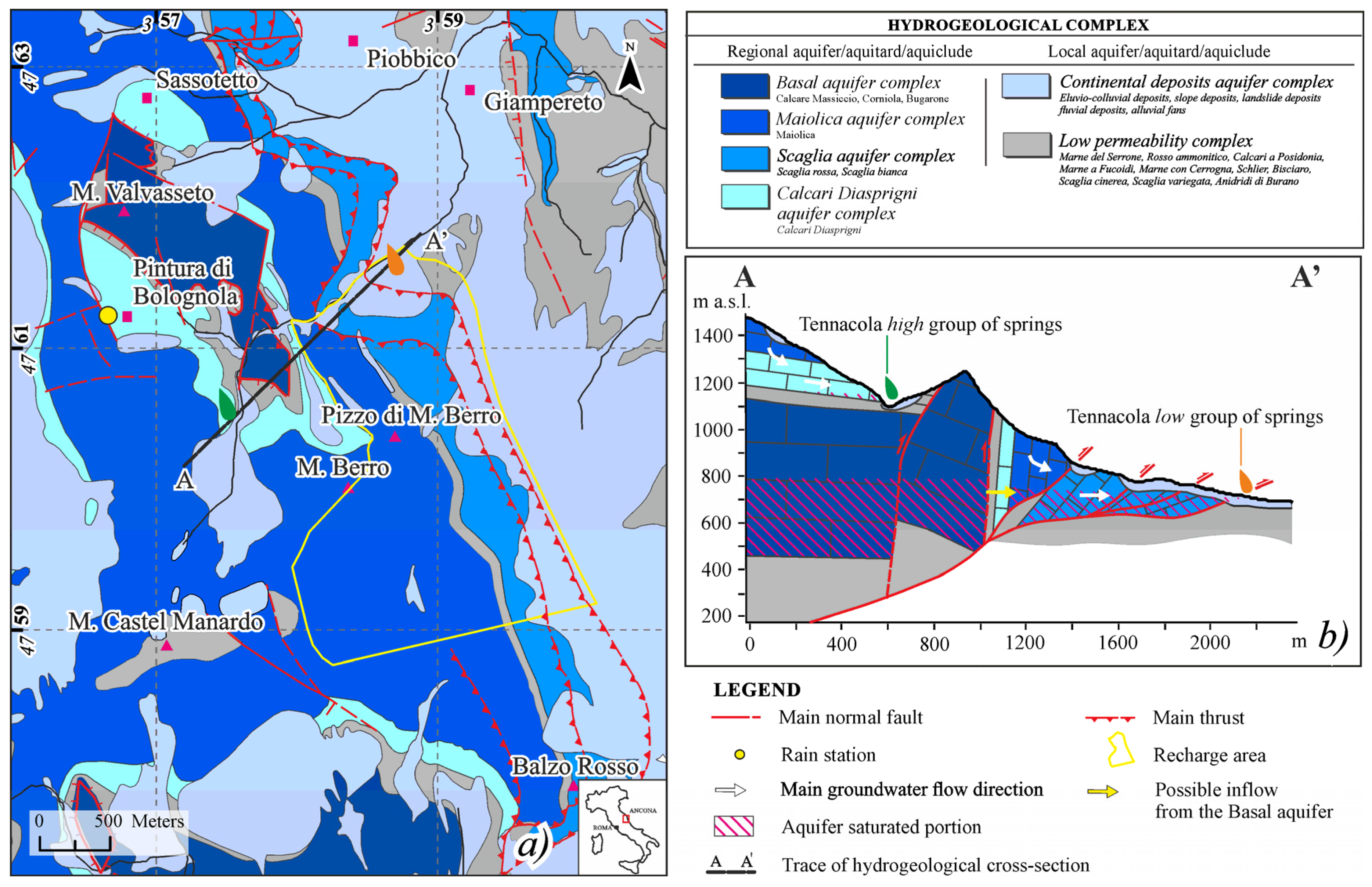
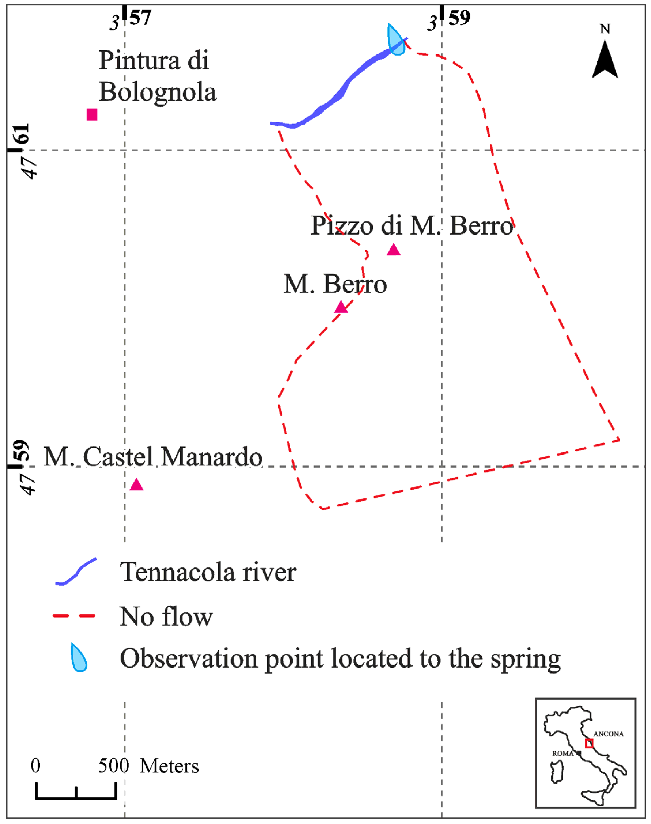
The study area is located in the northeast sector of the Sibillini Mountains, which is a calcareous massif located in the outermost part of the Umbria-Marche Ridge, and the study area corresponds to the mountainous portion of the Tennacola stream catchment between Mount Valvasseto (1526 m a.s.l.) and Mount Castel Manardo (1977 m a.s.l.) (Figure 1a).

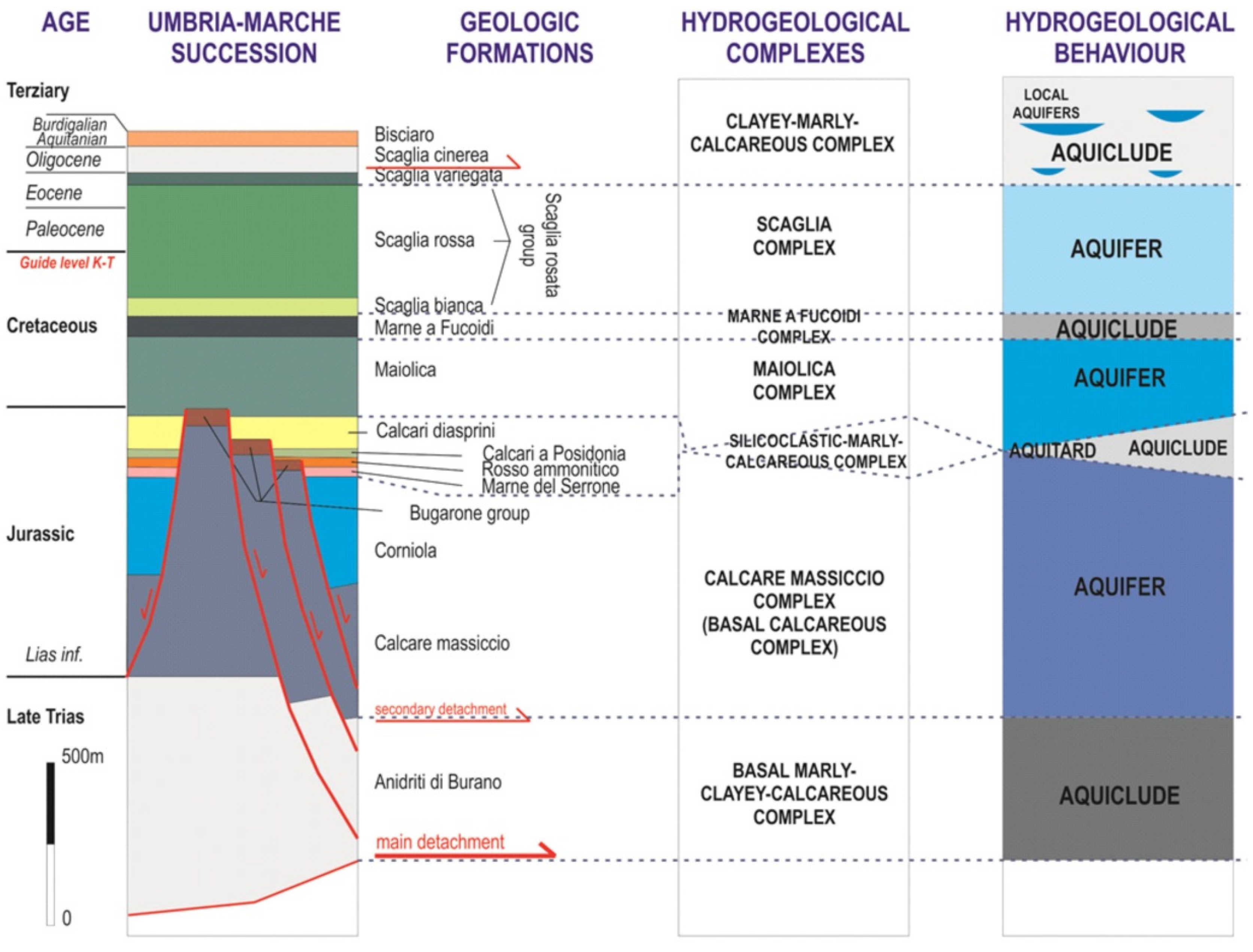
The outcropping geological formations are mainly composed of calcareous, marly and siliciclastic lithotypes (from Trias to Miocene in age) that belong to the Umbria-Marche Succession [41,42]. From bottom to top, the following formations can be observed (Figure 2):

-

Calcare massiccio formation (Hettangian-Pliensbachian p.p.): stratified limestone in tough blocks without noticeable vertical heterogeneities, approximately 700 m thick.

-

Bugarone group (Pliensbachian p.p.-Titonian p.p.): comprised of limestones and marly limestones with frankly greenish intercalations of marls in the marly calcareous facies; it outcrops only locally in substitution of the three previous formations, with an overall thickness of 30–40 meters.

-

Corniola formation (Sinemurian p.p.-Toarcian p.p.): finely stratified micritic limestones, with brown or light grey chert and with grey-green pelitic intercalations that are rather abundant both in the upper part and at the base; the thickness varies from 150 to 400 meters.

-

Bosso formation (Toarcian p.p.-Bajocian p.p.): comprised of a marly and marly calcareous unit with medium-thick strata (Marne del Serrone and Rosso Ammonitico); a third unit is made of limestones and marly limestones (Calcari a Posidonia). The overall thickness varies from 40 to 120 meters.

-

Calcari Diasprini formation (Bajocian p.p.-Titonian p.p.): limestones and cherty limestones with thick stratification; thickness can reach 100 meters.

-

Maiolica formation (Titonian p.p.-Aptian p.p.): whitish micritic limestones, in medium strata, with thin pelitic intercalations that increase towards the top of the formation. The thickness ranges from 150 and 400 meters.

-

Marne a Fucoidi formation (Aptian p.p.-Albian p.p.): the lower portion is made up of multicolored, closely layered marls and, subordinately, limestones that towards the top become cherty with frequent marly levels; 80–100 meters thick.

-

Scaglia rosata formation (Albian p.p.-Bartonian p.p.): limestones and marly limestones with polychrome chert, in medium and thin layers that vary in color from pink to red, (200–400 m);

-

Scaglia cinerea formation (Bartonian p.p.-Aquitanian p.p.): marly limestones, calcareous marls and clayey marls in thin layers (150–200 m).

-

Bisciaro formation (Aquitanian p.p.-Burdigalian p.p.): limestones, cherty limestones, marly limestones and calcareous and clayey marls, in medium and, sometimes, thick layers; the thickness ranges from 20 and 60 meters.

The current structural setting is the result of alternating compressive and extensive tectonic phases. The last configuration is a direct consequence of a former compressive phase that developed between the Miocene and early Pliocene that created east-verging folds and thrusts within the bedrock. Subsequently, a second phase, which had been active since the early Pleistocene, was characterized by an extensive regime associated with an intense tectonic uplift; this last phase generated vast active fault systems towards the Apennines, and the systems sometimes exploited the same old thrust planes [43,44]. The geological context described above is greatly complicated by the presence of the Sibillini thrust, which is characterized by a curved geometry and an approximately NW-SE direction (Figure 1a).

The presence of lithotypes with different permeabilities (aquifers/aquicludes/aquitards) allowed the formation of three main hydrogeological complexes that overlapped and are characterized by springs with different discharges and regimes (Figure 1a,b and Figure 2). The springs investigated herein emerge at different heights above the present thalweg, on the hydrographic right of the Tennacola stream.

Detailed surveys performed during the last three years have allowed the springs to be differentiated based on their proximities and hydrogeological characteristics (Figure 1b) into two main groups:

-

the Tennacola high group of springs; and

-

the Tennacola low group of springs.

The springs were captured and measured for groups of springs by the Tennacola Water Consortium (C.I.I.T.); The University of Camerino began detailed monitoring in 2014 by instrumenting the Tennacola low group of springs for the purpose of evaluating the single contribution.

In this study, only the Tennacola low group of springs, which is representative of the system under study, were considered. The Tennacola low group of springs emerges between approximately 700 m and 765 m a.s.l., at the contact between the Scaglia aquifer and the Scaglia Cinerea impermeable formation, and it represents the most important resource in the area, with discharges that range from 0.050 to 0.250 m³/s. In this case, the Scaglia aquifer likely forms a unique hydrogeological complex with the Maiolica aquifer, which is stratigraphically reversed here (Figure 1b). The Marne a Fucoidi aquiclude, which is usually interposed between the two aquifers, is partially elided or absent due to the compressive tectonics and the presence of the thrust plane. Moreover, preliminary water budgets led us to additionally hypothesize a minor contribution (approximately 10%) from the Basal aquifer on the western side of the area (Figure 1b).

2.2. Water Budget

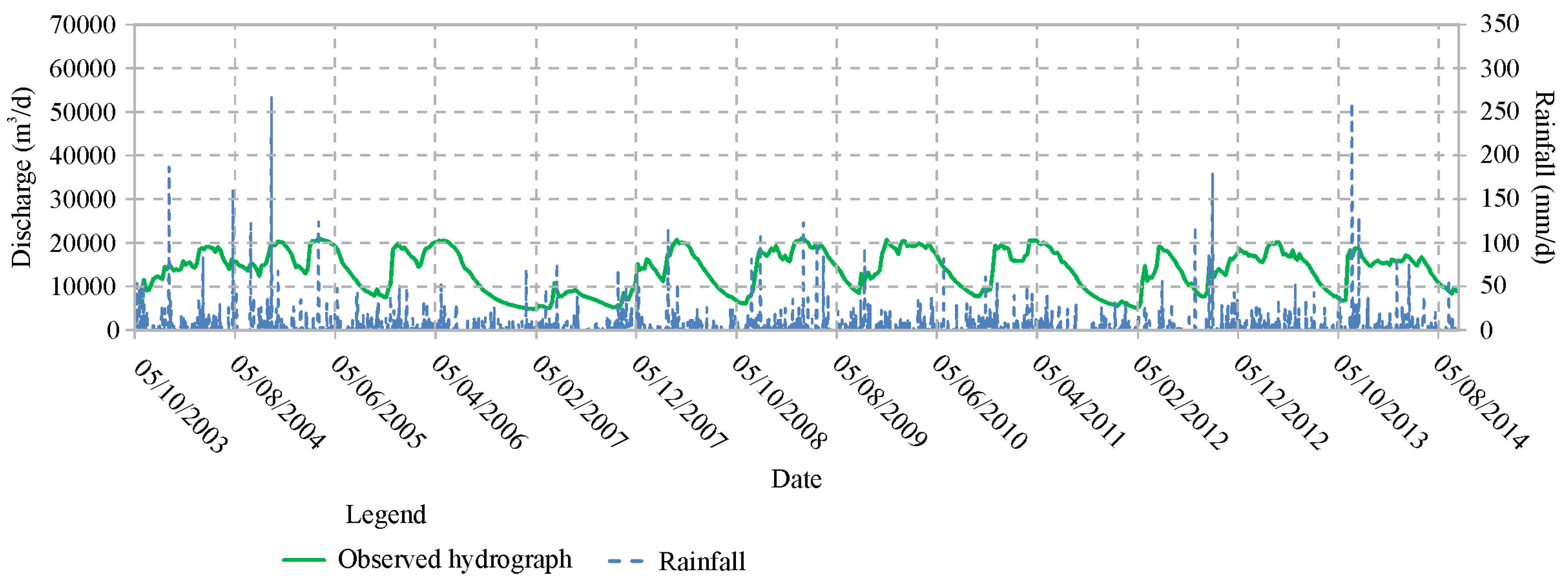
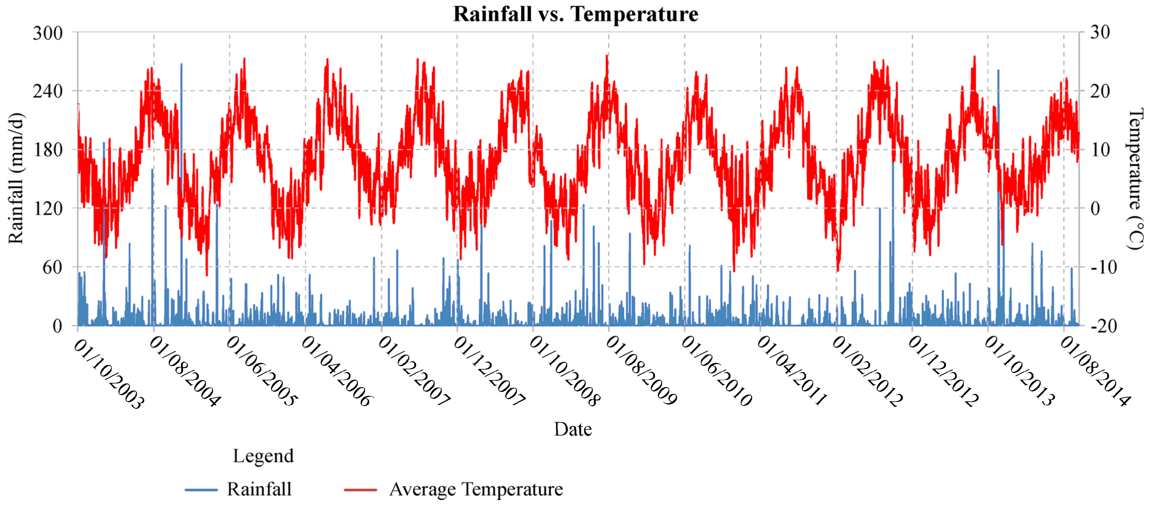
The water budget was evaluated for a period of 10 hydrologic years from 2004 to 2014 using meteorological data recorded at the Pintura di Bolognola weather station and fluvial and spring discharge data (Figure 3, Figure 4 and Figure 5).

The evapotranspiration was evaluated using different methods [45,46,47,48,49] to evaluate the differences in the methods.

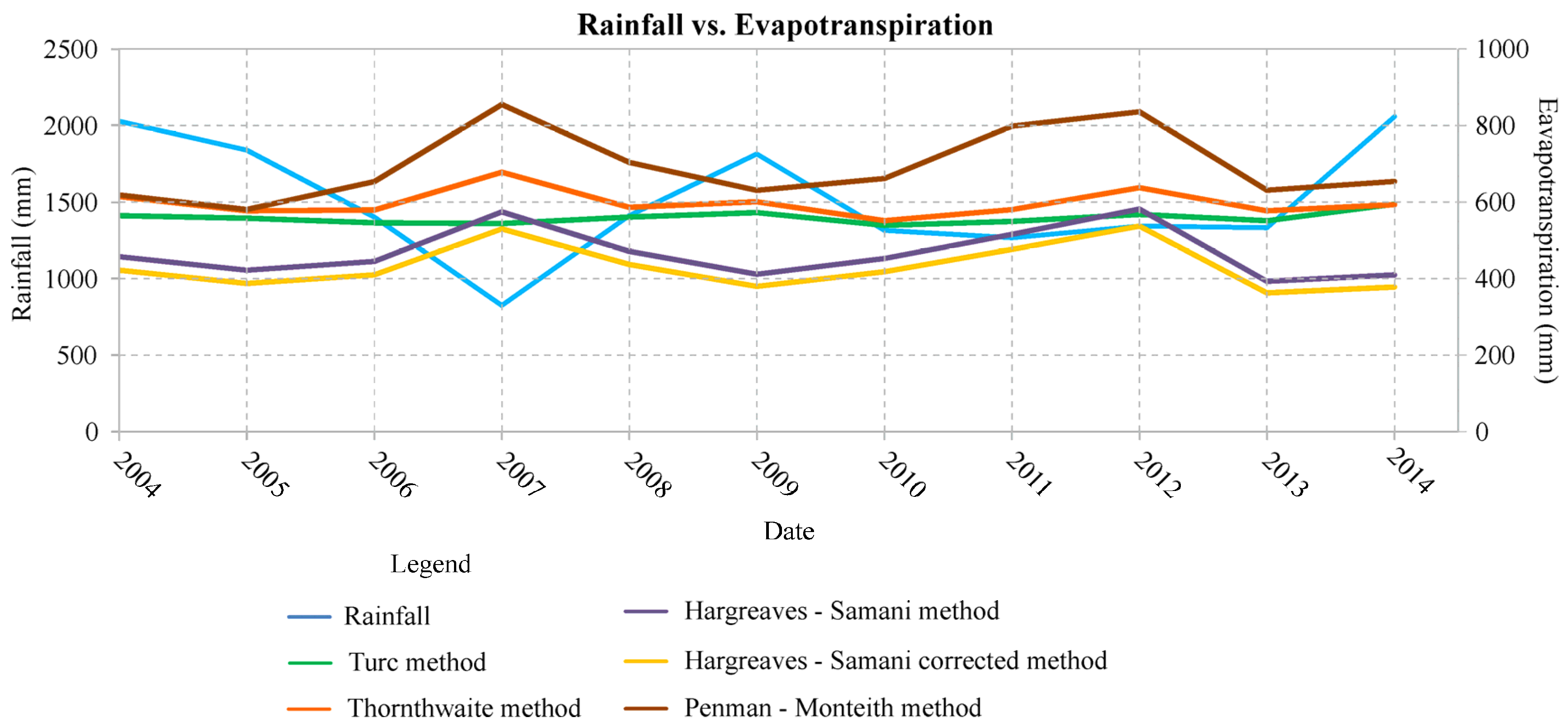
The results (

Table 1. Evapotranspiration assessment using different methods and next effective precipitation evaluation. P, rainfall; T, temperature; E_tr, real evapotranspiration; E_tp, potential evapotranspiration; E_t0, reference evapotranspiration; P_eff, effective rainfall.

Hydrologic Year	P (mm)	T (°C)	Turc		Thornthwaite		Hargreaves-Samani		Hargreaves-Samani Corrected		Penman-Monteith
			Etr (mm)	Peff (mm)	Etp (mm)	Peff (mm)	ET0 (mm)	Peff (mm)	ET0 (mm)	Peff (mm)	ET0,PM (mm)	Peff (mm)
2004	2027.80	7.91	507.55	1520.25	552.55	1475.25	411.53	1616.27	379.66	1648.14	556.48	1471.32
2005	1839.00	7.82	501.71	1337.29	519.13	1319.87	379.69	1459.31	348.50	1490.50	522.46	1316.54
2006	1401.40	7.85	490.86	910.54	521.31	880.09	400.34	1001.06	368.90	1032.50	588.04	813.36
2007	823.80	9.80	489.18	334.62	610.29	213.51	516.76	307.04	476.75	347.05	769.34	54.46
2008	1411.20	8.30	504.34	906.86	527.35	883.85	424.12	987.08	392.98	1018.22	633.10	778.1
2009	1814.40	8.26	514.93	1299.47	540.55	1273.45	369.99	1444.41	341.48	1472.92	567.63	1246.77
2010	1314.00	7.77	484.96	829.44	496.12	818.28	407.39	907.01	375.90	938.50	595.47	718.93
2011	1266.60	8.18	494.10	772.50	522.15	743.65	464.16	802.44	428.42	838.18	718.42	548.18
2012	1342.40	8.62	510.63	831.77	573.85	770.75	523.60	818.80	483.35	859.05	752.39	590.01
2013	1331.60	8.13	495.93	835.67	519.31	812.09	353.48	978.12	326.27	1005.33	567.77	763.83
2014	2058.00	8.74	534.84	1523.16	533.80	1523.40	368.47	1689.53	339.84	1718.16	588.36	1469.64
Mean value	1511.87	8.31	502.64	1009.23	537.86	974.02	419.96	1091.92	387.46	1124.41	623.59	888.29

) are comparable to those of other studies carried out at a larger scale [50]; in particular the evapotranspiration ranged from 390 mm/year to 624 mm/year (Figure 6) with an effective precipitation ranging from 890 mm/year to 1124 mm/year.

The methods of Turc and Thornthwaite provided similar average values of approximately 500 mm/year, while the daily Hargreaves-Samani and Penman-Monteith methods yielded average values of approximately 400 mm/year and 620 mm/year, respectively; the Penman-Monteith method, recommended by the Food and Agriculture Organization of the United Nations (F.A.O.), can be, however, a double-edged weapon because the greater amount of input measured data could lead to larger uncertainty. The evapotranspiration value was not considered during negligible conditions that avoid the evapotranspiration process [47].

The runoff was evaluated through the use of bibliographic and monitoring data; the first fluvial discharges were measured by Perrone [51], who considered river sections located downstream of the study area. Over the years, another analysis, made by the University of Rome La Sapienza [50,52,53], showed a negligible runoff.

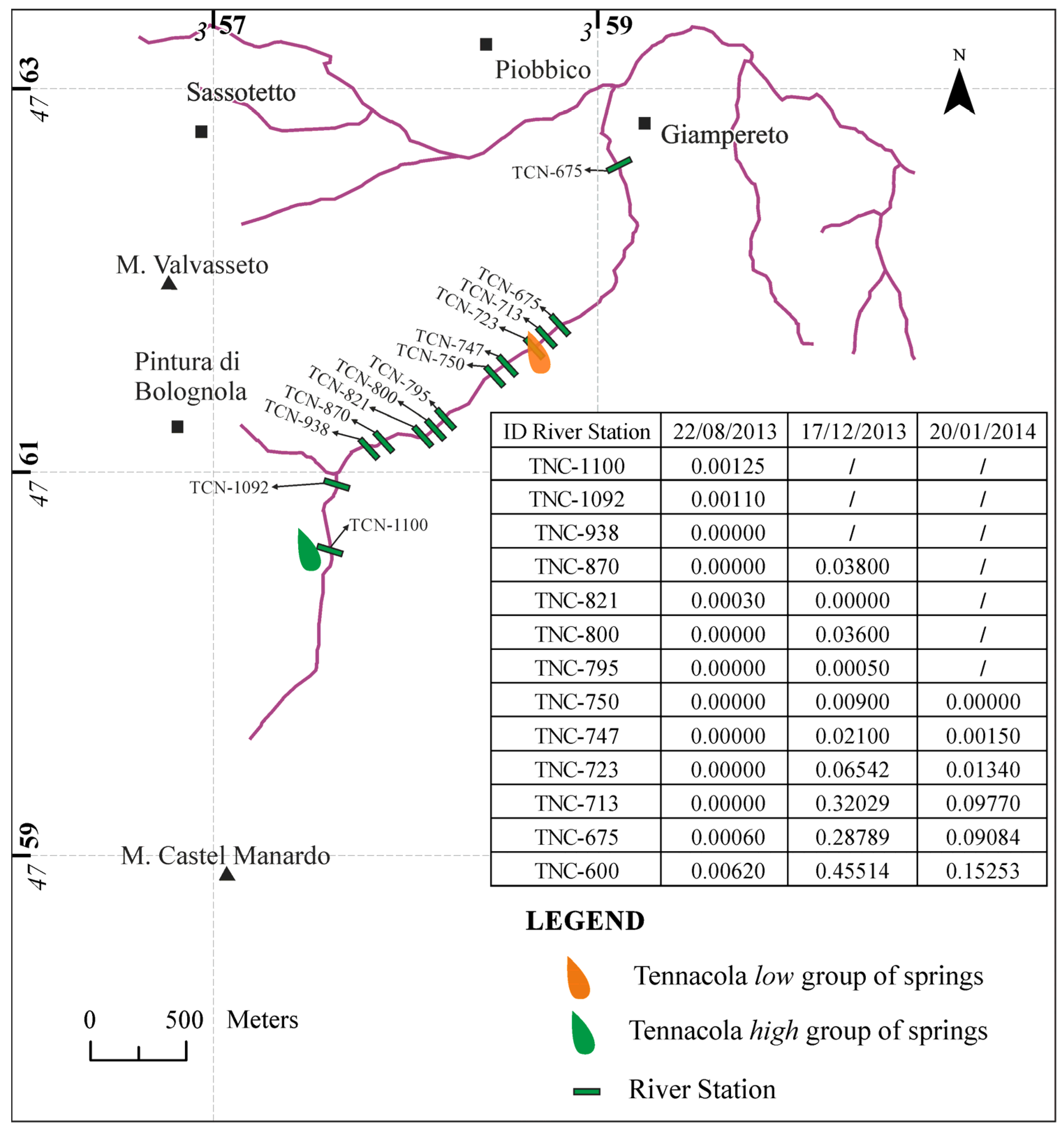
Three measurement campaigns were conducted by the University of Camerino along the Tennacola stream between August 2013 and January 2014 in order to monitor the river discharge during the dry and wet seasons (Figure 4). For the monitoring, 16 measuring stations were used that were evenly distributed from 1100 and 600 m a.s.l., which corresponded to the highest and lowest group of analyzed springs. The data collected during the summer periods (August 2013) showed that the river became nearly dry along the investigated reach. In fact, only limited sectors of the river (a few tens of meters) had discharges of 0.002–0.003 m³/s that, however, were suddenly absorbed by the large thicknesses of the coarse materials (pebbles and blocks) that form the riverbed. Slightly more significant discharges (approximately 0.006 m³/s) were recorded at the lowest station, which was located at an altitude of 600 m a.s.l. These conditions certainly persisted until the first half of October when, during the periodical surveys, no significant changes were observed.

The situation changed significantly after the heavy rainfall that was recorded in the area on 11, 12 and 13 November 2013. The second campaign of measurements (December 2013) showed significant increases in fluvial discharge. Although it was not possible to reach the first three stations (due to high snow avalanche and landslide hazards), the monitoring detected significant increases in the fluvial reach between 875 and 860 m a.s.l. However, these quantities were rapidly absorbed from the riverbed that, up to an altitude of 747 m a.s.l., showed considerable discharge variations, with alternating reaches completely dry or with reduced flows. The major increases were recorded starting from an altitude of 723 m a.s.l. (in correspondence with the Tennacola low group of springs), where the values reached 0.320 m³/s and then decreased significantly (0.287 m³/s) at the river station at 675 m a.s.l. (due to the large amounts of coarse materials in the river bed). After that, the flow increased again at the last station (altitude 600 m a.s.l.), where the fluvial discharge exceeded 0.450 m³/s. A similar trend was observed during the January 2014 measurement campaign.

The bibliographic and monitoring data showed negligible or no runoff, and any runoff accompanied snow melting and significant weather events (as confirmed by measurements made during December 2013); the river is therefore probably connected to the piezometric field, as observed at river station 713 (Figure 4), and flow under the debris is associated with the formation of a riverbed aquifer.

To elaborate the water budget, it was therefore decided to assume negligible runoff and apply a coefficient of potential infiltration (C.I.P.) of 95% [54]. The effective infiltration (

Table 2. Effective infiltration assessment using different methods for the period between 2004 and 2014.

Hydrologic Year	Parameter	Turc	Thornthwaite	Hargreaves-Samani	Hargreaves-Samani Corrected	Penman-Monteith
2004	P (mm)	2027.8	2027.8	2027.8	2027.8	2027.8
	Et (mm)	507.6	552.6	411.5	379.7	556.5
	Peff (mm)	1520.3	1475.3	1616.3	1648.1	1471.3
	R (mm)	76.0	73.8	80.8	82.4	73.6
	Ieff (mm)	1444.2	1401.5	1535.5	1565.7	1397.8
2005	P (mm)	1839.0	1839.0	1839.0	1839.0	1839.0
	Et (mm)	501.7	519.1	379.7	348.5	522.5
	Peff (mm)	1337.3	1319.9	1459.3	1490.5	1316.5
	R (mm)	66.9	66.0	73.0	74.5	65.8
	Ieff (mm)	1270.4	1253.9	1386.4	1416.0	1250.7
2006	P (mm)	1401.4	1401.4	1401.4	1401.4	1401.4
	Et (mm)	490.9	521.3	400.3	368.9	588.0
	Peff (mm)	910.5	880.1	1001.1	1032.5	813.4
	R (mm)	45.5	44.0	50.0	51.6	40.7
	Ieff (mm)	865.0	836.1	951.0	980.9	772.7
2007	P (mm)	823.8	823.8	823.8	823.8	823.8
	Et (mm)	489.2	610.3	516.8	476.8	769.3
	Peff (mm)	334.6	213.5	307.0	347.1	54.5
	R (mm)	16.7	10.7	15.4	17.4	2.7
	Ieff (mm)	317.9	202.8	291.7	329.7	51.7
2008	P (mm)	1411.2	1411.2	1411.2	1411.2	1411.2
	Et (mm)	504.3	527.4	424.1	393.0	633.1
	Peff (mm)	906.9	883.9	987.1	1018.2	778.1
	R (mm)	45.3	44.2	49.4	50.9	38.9
	Ieff (mm)	861.5	839.7	937.7	967.3	739.2
2009	P (mm)	1814.4	1814.4	1814.4	1814.4	1814.4
	Et (mm)	514.9	540.6	370.0	341.5	567.6
	Peff (mm)	1299.5	1273.9	1444.4	1472.9	1246.8
	R (mm)	65.0	63.7	72.2	73.7	62.3
	Ieff (mm)	1234.5	1210.2	1372.2	1399.3	1184.4
2010	P (mm)	1314.4	1314.4	1314.4	1314.4	1314.4
	Et (mm)	485.0	496.1	407.4	375.9	595.5
	Peff (mm)	829.4	818.3	907.0	938.5	718.9
	R (mm)	41.5	40.9	45.4	47.0	36.0
	Ieff (mm)	788.0	777.4	861.7	892.0	683.0
2011	P (mm)	1266.6	1266.6	1266.6	1266.6	1266.6
	Et (mm)	494.1	522.2	464.2	428.4	718.4
	Peff (mm)	772.5	744.5	802.4	838.2	548.2
	R (mm)	38.6	37.2	40.1	41.9	27.4
	Ieff (mm)	733.9	707.2	762.3	796.3	520.8
2012	P (mm)	1342.4	1342.4	1342.4	1342.4	1342.4
	Et (mm)	510.6	573.9	523.6	483.4	752.4
	Peff (mm)	831.8	768.6	818.8	859.1	590.0
	R (mm)	41.6	38.4	40.9	43.0	29.5
	Ieff (mm)	790.2	730.1	777.9	816.1	560.5
2013	P (mm)	1331.6	1331.6	1331.6	1331.6	1331.6
	Et (mm)	495.9	519.3	353.5	326.3	567.8
	Peff (mm)	835.7	812.3	978.1	1005.3	763.8
	R (mm)	41.8	40.6	48.9	50.3	38.2
	Ieff (mm)	793.9	771.7	929.2	955.1	725.6
2014	P (mm)	2058.0	2058.0	2058.0	2058.0	2058.0
	Et (mm)	534.9	533.8	368.5	339.9	588.4
	Peff (mm)	1523.2	1524.2	1689.5	1718.2	1469.6
	R (mm)	76.2	76.2	84.5	85.9	73.5
	Ieff (mm)	1447.0	1448.0	1605.1	1632.3	1396.2
Average	P (mm)	1511.9	1511.9	1511.9	1511.9	1511.9
	Et (mm)	502.6	537.9	420.0	387.5	623.6
	Peff (mm)	1009.2	974.0	1091.9	1124.4	888.3
	R (mm)	50.5	48.7	54.6	56.2	44.4
	Ieff (mm)	958.8	925.3	1037.3	1068.2	843.9

) ranged on average from 843.87 mm/year to 1068.19 mm/year. Considering the bibliographic [50,52] and monitoring data, a maximum effective infiltration of approximately 1068 mm/year was assumed.

A recession analysis of the springs was conducted examining their depletion curves for the period 2004–2014. The analysis showed that the system’s depletion constant ranged from 0.003 to 0.008 with an average value of 0.006. Based on those results, the groundwater recharge was estimated from the spring discharges for the same period [55].

The Tennacola low group of springs from 2004 to 2014 was characterized by a dynamic change in reserves of approximately 827,471 m³, with a recharge of approximately 55,515,801 m³ and an annual average flow of approximately 5,046,891 m³/year (

Table 3. Tennacola low group of springs budget analysis. Q₀, discharge at the beginning of the period measurement; Q_t, discharge at the time t; V₀, dynamic reserve at the beginning of the period; V_t, dynamic reserve at the end of the period; ΔV, dynamic reserve change during the water year; Q_ya, groundwater discharge volume during the water year; R, groundwater recharge.

Hydrologic Year	Initial Discharges		Dynamic Reserve		Dynamic Reserve Change	Discharge	Recharge
	Q0 (m3/s)	Qt (m3/s)	V0 (m3)	Vt (m3)	ΔV (m3)	Qya (m3)	R (m3)
2004	0.081405	0.167231	1,004,770.53	2,064,108.34	1,059,337.8	5,224,351	6,283,689
2005	0.163678	0.099915	2,020,254.57	1,233,234.84	−787,019.72	5,832,717	5,045,698
2006	0.094687	0.095703	1,168,703.87	1,181,246.24	12,542.367	5,484,057	5,496,599
2007	0.078592	0.063809	970,045.879	787,591	−182,454.88	2,407,626	2,225,171
2008	0.073567	0.087314	908,021.541	1,077,701.27	169,679.73	4,746,155	4,915,835
2009	0.073831	0.115963	911,288.695	1,431,319.19	520,030.49	5,599,006	6,119,037
2010	0.117108	0.097739	1,445,448.3	1,206,378.76	−239,069.54	5,530,212	5,291,143
2011	0.097566	0.096214	1,204,238.86	1,187,551.71	−16,687.148	5,501,548	5,484,861
2012	0.079799	0.144573	984,948.743	1,784,445.76	799,497.02	3,794,060	4,593,557
2013	0.153852	0.095275	1,898,976.22	1,175,969.27	−723,006.95	5,600,413	4,877,406
2014	0.086282	0.10367	1,064,962.68	1,279,584.59	214,621.92	4,968,184	5,182,806
Total value	1.100366	1.167406	13,581,659.9	14,409,131	827,471.09	54,688,330	55,515,801
Average value	0.092189	0.096703	1,137,882	1,193,595.12	55,713.56	4,971,666	5,046,891

).

2.3. Conceptual Model

Based on the geological and hydrogeological characteristics described so far, a conceptual model for the study area was defined (Figure 1a,b):

-

a western side, where the Maiolica and Calcare Massiccio aquifers are separated by an aquiclude comprised of the Bugarone, Calcari a Posidonia and Calcari Diasprigni formations: based on the water budget discussed in the previous section, a partial connection between the two aquifers (with a very limited contribution from the basal aquifer) was considered;

-

an eastern side, where the thrust plane and the underlying Scaglia cinerea low permeability formation, constitute an impermeable barrier;

-

a northern side, where the Tennacola low group of springs is located, and with no contribution from the Tennacola stream; and

-

a southern side, where inflow was excluded because of the presence of a structural underground water divide.

The main aquifer is comprised of the Maiolica and Scaglia formations; the Marne a Fucoidi formation, which is usually interposed between them, was not detected during the monitoring, probably because it has been partly erased by the thrust. For this reason, here it must be considered as an aquitard that produces a general delay in the flow of groundwater to the springs.

The spring hydrograph analysis confirmed the complexity of the whole system. The low value of the depletion constant, α = 0.006, and the curve homogeneity describe a well-defined catchment (also confirmed by the strict correlation between precipitation spring discharge) and a groundwater circuit that mainly occurs as a gradual flow through a widespread network of fractures and a low permeability matrix [56,57]. In relation to the features of the geological formations, the dimensions of the study area and the results from the spring hydrograph analysis, the equivalent continuum approach was applied in the present study, with the same value for the fractures and matrix system.

The geological and hydrogeological monitoring allowed a recharge area of 3.8 km² to be considered (Figure 1a); therefore, in relation to the water budget and annual discharge at the springs, the effective infiltration was determined to range from 70% to 80% of the mean yearly recharge.

The role of the river is uncertain. The fluvial discharge monitoring carried out during 2012–2013 evidenced that the river is completely dry for most of the year, except for a few days following snow melt and extreme rainfall events; this fact can be related to the high amount of coarse debris present along the river bed. Therefore, the river flow under the debris is probably connected to the groundwater flow.

2.4. Model Design

The numerical model related to the Tennacola low group of springs was developed using the FEFLOW [58], which is widely used to describe groundwater flow and transport processes in porous and fractured media.

As discussed in the previous sections, the model domain is very complex because of the presence of numerous lithological classes and structural elements. Therefore, the local contexts in the numerical model involve simplifications.

The study area can be divided into five different sectors (Figure 7):

-

Sector 1, which is characterized by two overlapping aquifer systems: the Maiolica aquifer (sMai) on the top and the Basal aquifer (sBas) below, which are separated by low permeability formations;

-

Sector 2, which corresponds to the Maiolica aquifer (sMai);

-

Sector 3, which is characterized by the Marne a Fucoidi aquiclude (sFuc);

-

Sector 4, which is characterized by the Scaglia aquifer (sScr); and

-

Sector 5, which corresponds to the valley floor of the Tennacola stream thick fluvial deposits (sTen).

The modeling approach used four different simulations of increasing complexity (Figure 7):

-

two zone model, M2Z (sBas, sMai-sFuc-sScr-sTen);

-

three zone model, M3Z (sBas, sMai-sFuc-sScr, sTen);

-

four zone model, M4Z (sBas, sMai-sScr, sFuc, sTen); and

-

five zone model, M5Z (sBas, sMai, sFuc, sScr, sTen).

The model domain, which was comprised of one layer, extended over an area of approximately 3.8 km² and was discretized into a mesh of 2085 elements and 2290 nodes. Because stratigraphic and water table data were missing in the study area, the initial piezometric surface was reconstructed using interpretative hydrogeological cross-sections, bibliographic data and the results of fluvial discharge monitoring carried out in the mountainous portion of the Tennacola stream.

2.5. Hydrogeological Properties

The hydrogeological parameters (

Table 4. The range of hydrogeological parameters for the five zones used in the analysis. K_xx,yy,zz = hydraulic conductivity for the different space orientations; S_y = specific yield; TR IN/OUT = transfer rate input/output; minimum (min), reference and maximum (max) values of hydrogeological parameters.

Model	Zone	Sector ID	Kxx (m/s)			Kyy (m/s)			Kzz (m/s)			Sy (-)			TR IN/OUT (1/day)
			Min	Ref	Max	Min	Ref	Max	Min	Ref	Max	Min	Ref	Max	Min	Ref	Max
M2Z	1	sBas	1e−08	1e−06	1e−05	1e−08	1e−06	1e−05	1e−09	1e−07	1e−06	0.008	0.01	0.05	1e−01	8.64e−04	1e+10
	2	sSca,sMai,sFuc,sTen	1e−04	5e−04	1e−03	1e−04	5e−04	1e−03	1e−05	5e−05	1e−04	0.002	0.005	0.01
M3Z	1	sBas	1e−08	1e−05	1e−03	1e−08	1e−05	1e−03	1e−08	1e−05	1e−03	0.001	0.005	0.1
	2	sSca, sMai,sFuc	1e−09	1e−07	1e−05	1e−09	1e−07	1e−05	1e−09	1e−07	1e−05	0.005	0.05	0.5
	3	sTen	1e−03	1e−02	1e−01	1e−03	1e−02	1e−01	1e−03	1e−02	1e−01	0.05	0.1	0.5
M4Z	1	sBas	1e−09	3.5e−07	1e−05	1e−09	5.8e−08	1e−05	1e−09	1.6e−07	1e−05	0.005	0.009	0.5
	2	sSca-SMai	1e−08	4e−05	1e−03	1e−08	1.6e−05	1e−03	1e−08	2.5e−05	1e−03	0.001	0.005	0.5
	3	sTen	1e−03	4.5e−03	1e−01	1e−03	1.7e−02	1e−01	1e−03	1.2e−02	1e−01	0.05	0.3	0.5
	4	sFuc	1e−08	1e−07	1e−05	1e−08	1e−07	1e−05	1e−08	1e−07	1e−05	0.001	0.002	0.1
M5Z	1	sBas	1e−09	3.5e−07	1e−05	1e−09	5.8e−08	1e−05	1e−09	1.6e−07	1e−05	0.005	0.009	0.5
	2	sSca	1e−06	1e−05	1e−03	1e−06	1e−05	1e−03	1e−06	1e−05	1e−03	0.01	0.05	0.5
	3	sTen	1e−03	4.5e−03	1e−01	1e−03	1.7e−02	1e−01	1e−03	1.2e−02	1e−01	0.05	0.3	0.5
	4	sFuc	1e−08	1e−07	1e−05	1e−08	1e−07	1e−05	1e−08	1e−07	1e−05	0.001	0.005	0.1
	5	sMai	1e−06	1e−04	1e−03	1e−06	1e−04	1e−03	1e−06	1e−04	1e−03	0.01	0.05	0.5

) were estimated from bibliographic data [59,60,61,62], in relation to the features of the study area. The calibration was focused on conductivity, specific yield and transfer rate parameters.

The range of hydrogeological parameters related to the five zones is shown in Table 4. The parameters have been made vary during the calibration process within a specific range (indicated with min and max values in Table 4) starting from a reference value (indicated with ref in the same table). The number of zones was progressively increased from two to five and the range was refined in relation to the results of previous simulations.

2.6. Boundary Conditions

The choice of boundary conditions (BC) followed the conceptual model described above (Figure 8). No-flow boundaries were used for the western, eastern and southern sides of the study area, but the Tennacola stream was represented using a constant head boundary (Cauchy BC). The infiltration was assumed to be time varying and was applied homogeneously to the entire study sector, which was assumed to be the recharge area. The numerous springs were grouped together and simulated using a Seepage Face (Dirichlet BC with a constraint), and the outflow from the model occurred only when the water table exceeded the elevation of the springs.

2.7. Model Calibration

The calibration was performed using the parameter estimation code PEST [63], which is an automated model calibration that uses an inverse parameter estimation process based on the Gauss-Marquardt-Levenberg method. This methodology allowed us to find an optimal parameter distribution to reduce the differences between the observed and simulated data by minimizing the sum of the squared weighted residuals.

The residual analysis allowed the quality of the model to be evaluated from statistical indexes such as the sum of squared weighted residuals, Φ, and the standard error, σ [20,64].

The sum of the squared weighted residuals between the observed and simulated values is expressed by the following relationship:

$$\mathsf{\Phi }={\left(\mathrm{c}-{\mathrm{c}}_0\mathrm{J}\left(\mathrm{b}-{\mathrm{b}}_0\right)\right)}^{\mathrm{t}}\mathrm{Q}\left(\mathrm{c}-{\mathrm{c}}_0\mathrm{J}\left(\mathrm{b}-{\mathrm{b}}_0\right)\right)={\displaystyle \sum }_{\mathrm{i}=1}^{\mathrm{m}}\left[{\mathrm{w}}_{\mathrm{i}}\left({\mathrm{c}}_{\mathrm{i}}-{\mathrm{c}}_{\mathrm{i}}^{\text{'}}\right)\right]={\displaystyle \sum }_{\mathrm{i}=1}^{\mathrm{m}}{\left({\mathrm{w}}_{\mathrm{i}}{\mathrm{r}}_{\mathrm{i}}\right)}^2$$

(1)

where w_i is the weight of the ith-observation; ${\mathrm{c}}_{\mathrm{i}}$ is the ith-observation; ${\mathrm{c}}_{\mathrm{i}}^{\text{'}}$ is the simulated value corresponding to ${\mathrm{c}}_{\mathrm{i}}$; and ${\mathrm{r}}_{\mathrm{i}}$ is the residual value.

The standard error can be calculated starting from the variance σ_r² [64]:

$${{\mathsf{\sigma }}_{\mathrm{r}}}^2=\frac{{\mathsf{\Phi }}_{\text{min}}}{\left(\mathrm{n}-\mathrm{m}\right)}$$

(2)

where ${\mathsf{\Phi }}_{\text{min}}$ is the minimum objective function; n is the observations number; and m is the number of adjustable parameters.

The square root of the previous equation gives the standard error, σ:

$$\mathsf{\sigma }=\frac{\sqrt{{{\mathsf{\sigma }}_{\mathrm{r}}}^2}}{{\mathrm{w}}_{\mathrm{i}}}$$

(3)

The aforementioned indexes cannot adequately indicate the convergence of a model, especially as the number of adjustable parameters increases. To ensure a greater precision, four information criteria were employed [20,35,36,37,64,65]:

$$\text{AIC}=\mathrm{n}\ln \left({\mathsf{\sigma }}_{\mathrm{r}}^2\right)+2\mathrm{k}$$

(4)

$$\text{AICc}=\text{AIC}+\frac{2\mathrm{k}\left(\mathrm{k}+1\right)}{\mathrm{n}-\mathrm{k}-1}$$

(5)

$$\text{BIC}=\mathrm{n}\ln \left({\mathsf{\sigma }}_{\mathrm{r}}^2\right)+\mathrm{k}\ln \left(\mathrm{n}\right) \text{and}$$

(6)

$$\text{KIC}=\left(\mathrm{n}-\left(\mathrm{k}-1\right)\right)\ln \left({\mathsf{\sigma }}_{\mathrm{r}}^2\right)-\left(\mathrm{k}-1\right)\ln \left(2\mathsf{\pi }\right)+\text{ln}\left|{\mathrm{J}}^{\mathrm{t}}\text{QJ}\right|$$

(7)

where k is the number of estimable parameters; J is the Jacobian matrix; Q is the weight matrix; and J^tQJ is the normal matrix.

If the statistics for a model with few parameters are better than a model with more parameters, it is preferable to select the model with few parameters, unless there is no information on the validity of the more complex model [20].

These parameters are usually evaluated through the difference Δ_j of the AIC, which is also generally used to indicate differences in the other parameters, BIC and KIC [37]. This value is then used together with the Akaike weight:

$${\text{AIC w}}_{\mathrm{j}}=\frac{\text{exp}\left(-\frac{1}{2}·{\mathsf{\Delta }}_{\mathrm{j}}\right)}{{{\displaystyle \sum }}_{\mathrm{j}=1}^{\mathrm{R}}\text{exp}\left(-\frac{1}{2}·{\mathsf{\Delta }}_{\mathrm{j}}\right)}$$

(8)

where Δ_j is the difference of the AIC of a specific model to the smallest AIC from all of the considered models.

The value w_j indicates the best model among all of the evaluated models [37]. The difference value is inversely proportional to the weight w_j, and for low values of the weight, the probability that the considered model is the best is null.

The good fit between the simulated and observed data can be graphically evaluated through the correlation coefficient, R [20,63]:

$$\mathrm{R}=\frac{{{\displaystyle \sum }}^{\text{}}\left({\mathrm{w}}_{\mathrm{i}}{\mathrm{c}}_{\mathrm{i}}-\mathrm{m}\right)\left({\mathrm{w}}_{\mathrm{i}}{\mathrm{c}}_{\mathrm{i}}^{\prime }-{\mathrm{m}}^{\prime }\right)}{{\left[{{\displaystyle \sum }}^{\text{}}\left({\mathrm{w}}_{\mathrm{i}}{\mathrm{c}}_{\mathrm{i}}-\mathrm{m}\right)\left({\mathrm{w}}_{\mathrm{i}}{\mathrm{c}}_{\mathrm{i}}-\mathrm{m}\right){{\displaystyle \sum }}^{\text{}}\left({\mathrm{w}}_{\mathrm{i}}{\mathrm{c}}_{\mathrm{i}}^{\prime }-{\mathrm{m}}^{\prime }\right)\left({\mathrm{w}}_{\mathrm{i}}{\mathrm{c}}_{\mathrm{i}}^{\prime }-{\mathrm{m}}^{\prime }\right)\right]}^{1/2}}$$

(9)

where ${\mathrm{c}}_{\mathrm{i}}$ is the ith-observation value; ${\mathrm{c}}_{\mathrm{i}}^{\text{'}}$ is the model-generated counterpart to the ith-observation value; m is the mean of the weighted observed values; ${\mathrm{m}}^{\prime }$ is the mean of the weighted model-generated values; and w_i is the weight associated with the ith-observation.

The correlation coefficient is independent of the number of observations and the uncertainty level associated with the observations.

The PEST software allows the sensitivity of the selected parameters against the observed data to be evaluated. The PEST sensitivity for a generic parameter i is calculated as follows [63]:

$${\mathrm{s}}_{\mathrm{i}}=\frac{\sqrt{{\left({\mathrm{J}}^{\mathrm{t}}\text{QJ}\right)}_{\text{ii}}}}{\mathrm{m}}$$

(10)

where m is the number of observations with a nonzero weight.

The composite sensitivity s_j (related to observation j) is instead calculated as follows [63]:

$${\mathrm{s}}_{\mathrm{j}}=\frac{\sqrt{{\left\{\mathrm{Q}\left({\mathrm{J}}^{\mathrm{t}}\mathrm{J}\right)\right\}}_{\text{jj}}}}{\mathrm{n}}$$

(11)

where J^tJ is the Hessian matrix; j is the number of observations; and n is the number of adjustable parameters.

The model calibration was performed using the spring discharge values from 2004 and 2014. In particular, automatic inverse modeling was carried out starting from the simple model (M2Z) to obtain the more complex model (M5Z) that had a larger number of adjustable parameters. The best model was finally chosen based on the derived statistical indexes.

3. Results

3.1. Uncertainty Analysis

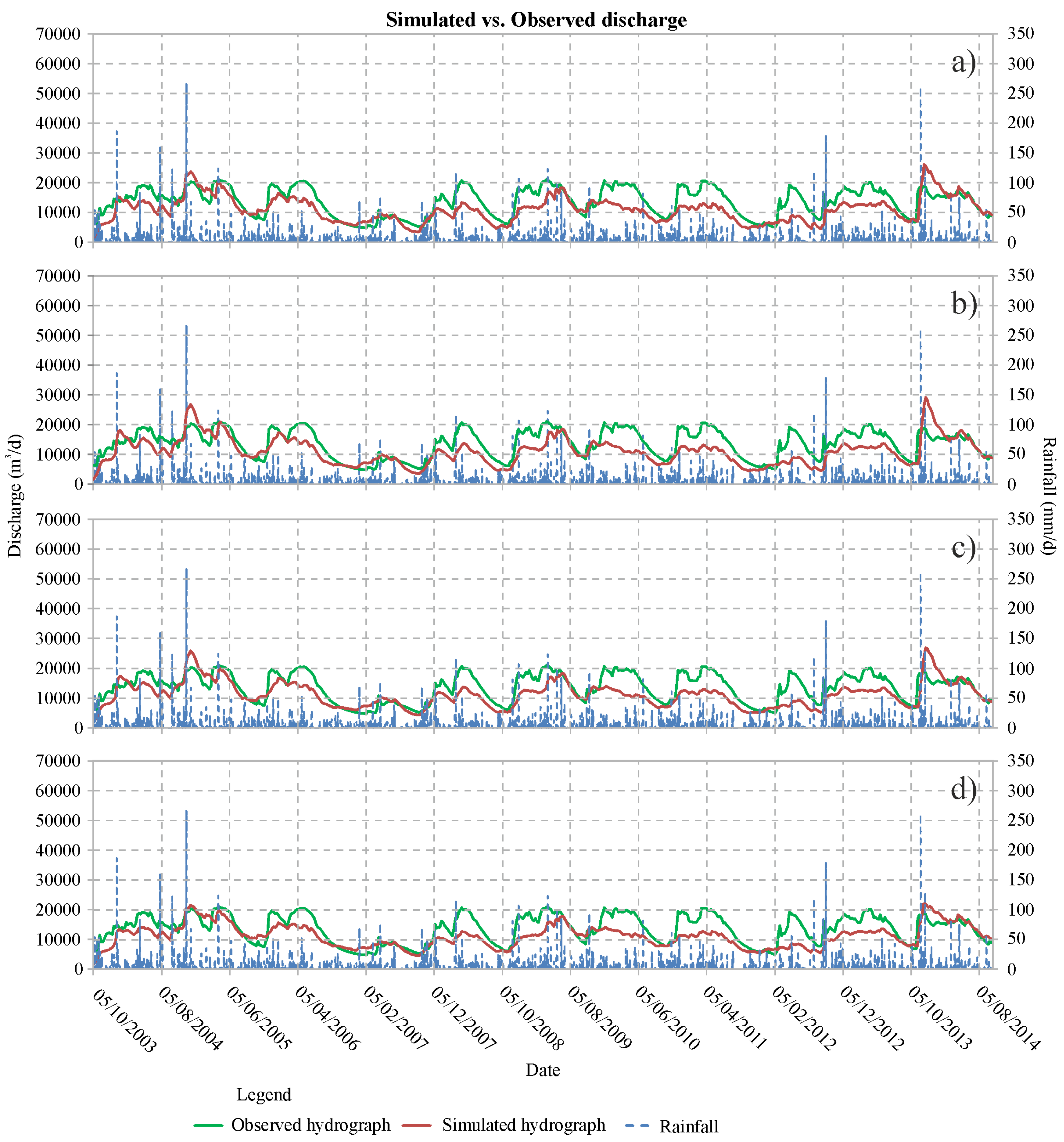
The uncertainty analysis was performed using four models with increasing complexity, with a minimum of 10 to a maximum of 22 adjustable parameters.

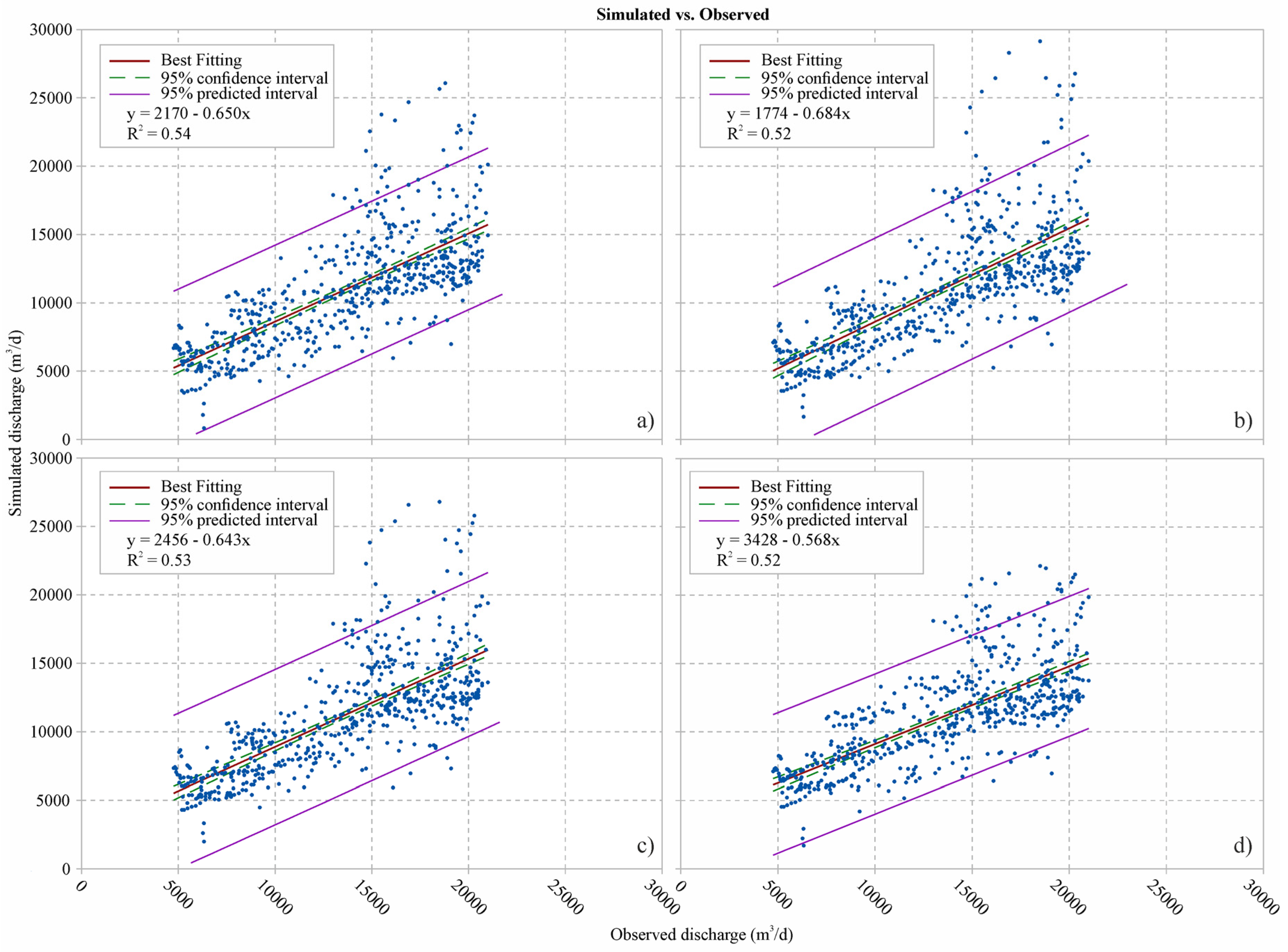
Figure 9 shows the simulated vs. observed discharges for all of the models.

Table 5. Statistical index derived from PEST analysis. ME_w, Average value of the weighted residuals; MAE_w, Absolute average value of the weighted residuals; σ_r², variance of weight residuals; σ_w, standard deviation; Φ (SSWR), sum of squared of the weighted residuals; R, correlation index.

Model	MEw	MAEw	σr2	σ	Φ	R
M2Z	−0.300	0.390	0.14	0.37	133	0.73
M3Z	−0.371	0.509	0.40	0.60	225	0.72
M4Z	−0.556	0.764	0.59	0.80	517	0.73
M5Z	−0.550	0.740	0.55	0.74	491	0.72

shows the results from the application of the main statistical indexes to the weighted residuals of each model. The weight used was evaluated considering the inverse of the standard deviation from the PEST analysis [20,66]. The reference variance should therefore be equal to 1 [20,63]; lower values represent a good fit between simulated and observed data, and higher values indicate a bad fit.

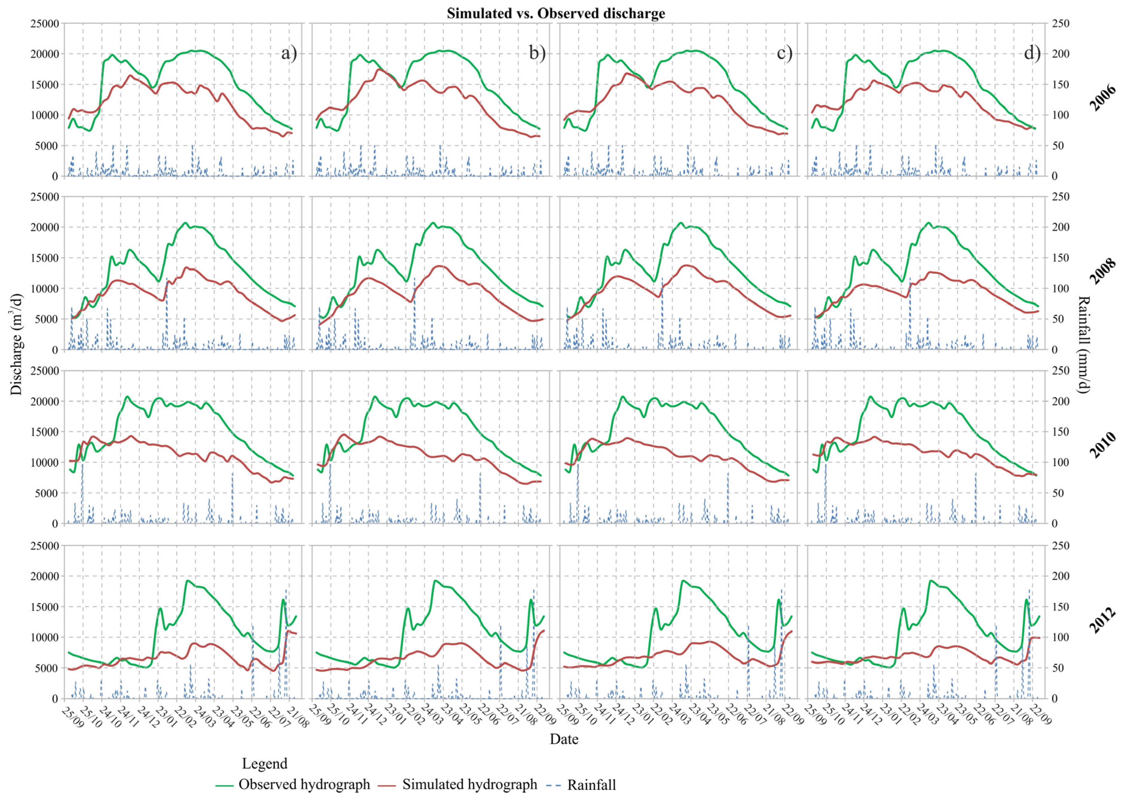
A detailed comparison between the simulated and observed hydrographs was made for the hydrologic years 2006, 2008, 2010 and 2012 (Figure 10); the figure shows that all of the models exhibited a similar trend and lack in the discharge (

Table 6. Difference between simulated and observed total discharge for the single year considered (ΔQ).

Model	2006	2008	2010	2012
	ΔQ (m3)	ΔQ (m3)	ΔQ (m3)	ΔQ (m3)
M2Z	1,119,329	1,428,274	1,489,013	1,343,655
M3Z	1,035,046	1,455,953	1,534,658	1,403,962
M4Z	1,054,714	1,284,587	1,538,168	1,258,872
M5Z	978,568	1,353,970	1,313,571	1,239,845
Average	1,046,914	1,380,696	1,468,853	1,311,584

).

The regression analysis showed a bad fit between the simulated and observed data based on the slope of the best fit line (Figure 11).

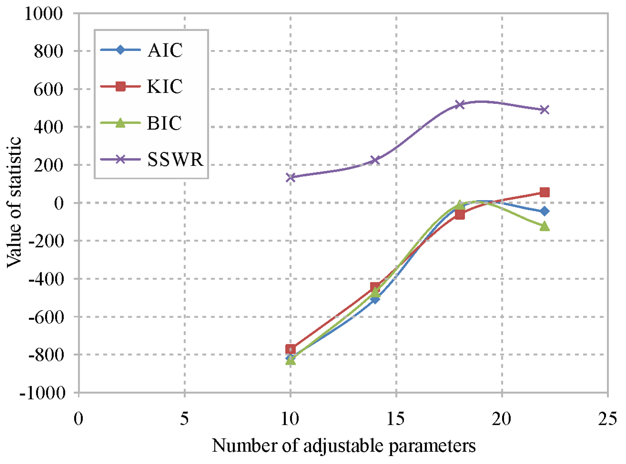
The analysis of the AIC, BIC and KIC coefficients allowed a determination of the best of the four proposed configurations: the coefficient AICc, in this case equal to AIC, was not considered. The information criteria show relative values, and the absolute values are nonsense; the scale of the y-axis in Figure 12 is therefore omitted. Finally, the Akaike weight (Equation (8)) was calculated to evaluate the likelihood of the models; values of 100% indicate the best model, and a value close to zero indicates a negligible model (

Table 7. Difference of the Akaike information criterion (AIC), Bayesian information criterion (BIC), and Kashyap’s information criterion (KIC) values and likelihood of the flow models from the Akaike Weights (AIC w_i).

Model	AIC	KIC	BIC	AIC wi
M2Z	0	0	0	1.00
M3Z	310.85	328.26	357.71	0.00
M4Z	797.66	710.75	817.64	0.00
M5Z	775.75	827.97	706.83	0.00

).

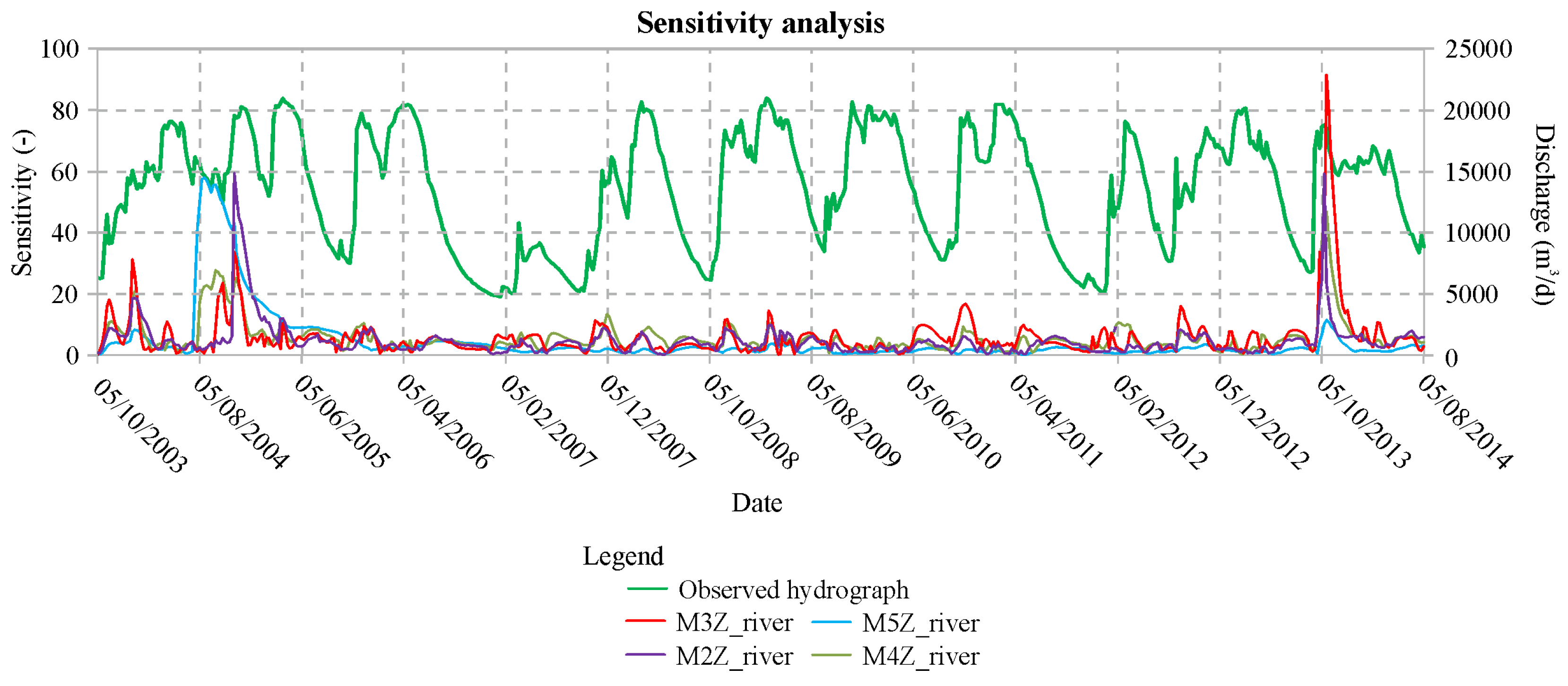
3.2. Sensitivity Analysis

The dimensional sensitivity was evaluated in relation to the observation group for each of the considered models (Figure 13).

The sensitivity analysis was very useful for evaluating the capacity of the models to represent the observed data.

For the proposed models, the sensitivity analysis showed comparable trends, but in particular the value was higher for the model with few parameters. In general, increasing the number of adjustable parameters decreased the sensitivity to the observation data within the model calibration [34].

All the proposed models showed a higher sensitivity for the observations matching the rainfall peaks (i.e., those of 5 August 2004 and 5 October 2013). In more detail, the models with three and four zones showed a higher sensitivity for the peak of rainfall on 5 October 2013, but the models with two and five zones were more sensitive for the peak on 05 August 2004.

4. Discussion

Based on the aforementioned analyses, it was possible to evaluate the goodness of the proposed models (Table 5). The variance, which was less than 1 in all of the considered models, indicates a good correspondence; the lowest value, in particular, corresponds to the model with two zones and a limited number of adjustable parameters. On the contrary, R, which was constant for all of the models, is apparently lower than the recommended value [66]. This result was also confirmed by the scatterline graph, in which the slope of the best-fit line was different than 1 (Figure 11). Even the simulated hydrographs (Figure 9) for all of the models had average errors from 0.038 and 0.040 m³/s, which were too high with respect to the observed discharges at the springs. The error is comparable among the models but slightly increases with the number of zones (and consequently with the number of adjustable parameters); this is due to the problem of equifinality, in which increasing the parameter space can increase the number of optimum solutions available and reducing the performance of all “optimums” [67]. As a consequence, the model with two zones and a low number of adjustable parameters remained the most suitable among the models investigated in relation to the available data. The analysis of the AIC, BIC and KIC parameters confirmed these results.

In addition, the AIC w_j, which was 100%, confirmed the goodness of the model with two zones among the models tested; on the contrary, the other models had values close to zero (Table 7). Engelhardt et al. [34] carried out an analysis of the significance of the BIC, KIC and AIC parameters. The first two parameters indicated that the best model had the lowest number of adjustable parameters, whereas AIC indicated that the best model had a higher number of parameters; the Akaike weight definitively confirmed the result expressed by the AIC parameter. However, because AIC ignores the potential error related to the geometry of the model, the authors stated that the choosing the KIC parameter could be the best solution, which confirmed the result achieved by [40]. Foglia et al. [30] conducted a multi-model analysis using AIC and BIC supported by a cross-validation, and they concluded that both information criteria selected the same optimal model with only three adjusted parameters.

The solution obtained in the present study could be related to the use of a single type of observational data; in fact the information criteria considers different model as optimal if a large number of observational data are available [34].

The detailed analyses carried out for single hydrologic years (Figure 10) instead showed good approximations of the hydrograph shape (discrete spatial distribution of the hydrogeological parameters); nevertheless, the simulated discharge showed a general underestimation in the observed discharge of approximately 1,500,000 m³/year on average (Table 6).

The selected model simulated a mean annual discharge of approximately 44,021,000 m³ over the entire period of investigation, but the mean annual discharge calculated by means of the spring hydrograph analysis and water budget, on the other hand, indicated a value of 55,515,801 m³. The results confirmed that infiltration in the study area plays a very important role because it feeds approximately 80% of the total discharges to the springs, and, as a consequence, approximately 20% should come from a neighboring aquifer.

5. Conclusions

The analysis was conducted by increasing complexity through increasing the number of adjustable parameters using the FEFLOW computer program and PEST automatic calibration; for each of the models under evaluation, the differences between the simulated and observed data were evaluated using the main statistical index and information criteria to evaluate the associated errors and uncertainties. The optimal model was evaluated using the differences between the simulated and observed water budgets to understand the goodness of the hypothesized conceptual model.

All of the models under consideration had small values of the main statistical index as well as those for the reference variance and the correlation index, which highlights the complexity of the geometry that controls the flow at the springs. The differences between observed and simulated data ranges, on average, between 0.038 and 0.040 m³/s; therefore, it seems probably high compared to the discharges at the springs. In relation to the four models evaluated, the information criteria in parallel with the Akaike weight identified the model with two zones, i.e., the model with the smallest number of adjustable parameters, to be the most suitable. Using that model, a total discharge for the whole period 2004–2014 of approximately 44,021,000 m³ was determined, compared with the average total observed at the springs of approximately 54,688,330 m³, which implied a contribution from infiltration of approximately 80% and a minor contribution of approximately 20% that was probably derived from the nearby basal aquifer on the western side of the area.

The comparison between the simulated and observed spring hydrographs showed a good shape correspondence but a general overestimation of the discharge, which indicates a good correspondence with the rainfall time series and consequently with the estimated water budget and a probably incorrect extension of the aquifer structure. The statistical analysis showed similar results with comparable discharge differences for each model, which indicated the same lack in available data independent of the geometrical model. In conclusion, the study confirmed that recharge contributes more than half of the total outflow at the springs but is not able to completely feed the springs, and it is necessary to invoke an external contributor, which is probably flow from the close Basal aquifer on the western side.

In conclusion, the aim of the paper would be not to provide a definitive solution, rather to foster debate and restrict uncertainty about assessment of different alternative models. Therefore the study presented is preliminary and designed to assess, in relation of available data, the real extension of the model. The analysis allowed an understanding of the uncertainties and errors associated with the hypothesized conceptual model in relation to the available data and its consequent limitations, showed the necessity of acquiring new data (e.g., new fluvial discharge monitoring, at least once per year, refining the measured discharges at the springs using the instruments installed by the University of Camerino in 2014 and geochemical surveys) and modifying the conceptual model (e.g., extending the study area) in order to improve and verify the achieved results.