The Effect of Energy Constraints on Water Allocation Decisions: The Elaboration and Application of a System-Wide Economic-Water-Energy Model (SEWEM)

Abstract

Worldwide, demand for water, energy, and food are on the rise due to population and industrial growth. Because of such increasing demands and in spite of the limitedness of key resources, more efficient ways to meet these demands become obligatory. Especially considering the multiple interlinkages between water, energy, and food/livelihood systems, an integrated management of key resources such as water, land, and energy deems essential for realizing synergetic efficiencies, for consistent policy decisions, and for sustainable development, in particular across the river basins of the world. Therefore, the general framework of a system-wide economic-water-energy model (SEWEM), which is applicable across river basins and adjustable to different spatial scales such as sub-catchments, is presented here to meet the demands for an effective analytical tool in dealing with water-energy-food/livelihood nexus challenges. Previous hydro-economic models often ignored energy requirements, for instance, for irrigation water supply, as well as energy supply constraints, which recurrently might have led to an overestimation of the optimal levels of ground and surface water uses. The SEWEM was developed to address this gap and analyze how optimal levels of surface and groundwater uses, as well as on irrigation and power production benefits, change in response to the consideration of energy supply constraints and energy requirements for water pumping and other agricultural production operations. This is illustrated for the case of the Aral Sea Basin (ASB) in Central Asia, where surface and groundwater supplies heavily depend on pumping and thus on energy availability. The findings underlined the overestimations of optimal water uses by a hydro-economic model that neglects energy constraints. Moreover, geographical conditions have affected the changes in optimal ratios of surface and groundwater uses and water distributions across the river basin when energy restrictions are taken into account. The results confirmed the importance of the consideration of energy constraints for the assessment of optimal water and land uses, and the essential role of an integrated analysis of water, energy, and food/livelihood systems for better-informed policy-making. Despite the added value of the SEWEM that can consider energy system constraints, further fine-tunings would make it even more relevant for addressing additional questions related to basin management. For example, improvements can be expected through considering the system dynamics, ecological aspects, income distribution effects, trade relationships, and institutional restrictions.

1. Introduction

Gaining food, water, and energy security for the ever-increasing population and expanding economies worldwide has never become such a great challenge as nowadays [1,2,3,4,5,6,7]. Several United Nations Sustainable Development Goals (SDGs) underscore this intention by setting the targets of increasing the number of population with adequate water and energy access (SDGs 6 and 7), reducing the negative consequences of water and climate abnormalities (SDG 13), and adapting technologies to secure food supply and reduce malnutrition and hunger (SDG 2) [8]. It has thus been acknowledged once more that an efficient use of the scarce water and energy resources is of the utmost importance to ease the current and future insecurity of food supply and reach the target of sustainable economic growth [6,9,10].

Economic analysis and modeling tools play a key role in assessing the efficient use of resources [9,11,12,13,14,15]. However, in spite of the close interlinkages between water, energy, and food/livelihood management systems, the management of these systems by separate ministries and institutions, as typical in many countries, have resulted in conflicting decisions [5]. A well-known, but not the only example, is the conflict over water sharing between hydropower generation and irrigation [16,17]. Although hydropower generation does not require a consumptive water use (except to compensate for evaporative losses from reservoirs), differences in seasonal water demands for hydropower generation and agriculture production are at the core of cross-sectoral conflicts. For instance, higher demands for energy during cold winter months, which would require water releases during winter periods, would reduce water availability for meeting peak irrigation water demands during summer periods [17,18]. On the other hand, synergistic examples of energy and food production system development do exist. For instance, irrigation operations and technological modernizations usually go hand in hand with a higher energy consumption, while energy production may depend on a biofuel-based production (agricultural byproducts, biofuel crops, etc.) [5,9,19]. Considering the strong interactions and interdependences of water, energy, and food production/livelihood systems, an integrated assessment and management of these systems should be at the center of policies on a sustainable use of scarce resources for economic growth.

Owing to the frequent occurrence of a separate management of water, energy, and food/livelihood systems, most of the existing water-economic models do not consider water demand for energy generation (except hydropower) or energy needs to ensure water supply for food production [15]. At the same time, energy planning models have focused on energy production and its distribution across sectors, but did not usually consider the dependence of energy production on water consumption or energy requirements for surface and ground water extraction through pumping [20,21,22]. More recently, integrated modeling tools that are capable of considering water and energy systems simultaneously have been developed [6,10]. Yet, these models aim at minimizing the gap between supply and demand for water and energy. Thus, despite a focus on water and energy flows in a production system, a cost-benefit analysis of water and energy provision and uses together has not been thoroughly considered yet, although being of high relevance to decision-makers and planners alike. Therefore, a general framework for a system-wide economic-water-energy model (SEWEM) was developed for addressing an integrated economic assessment of highly interlinked water, energy, and food/livelihood systems.

While elaborating an analytical tool capable of assessing the multiple challenges related to the water-energy-food/livelihood nexus, the focus here is on a detailed presentation and description of the structure of the SEWEM developed. For showing the relevance and importance of taking into account energy constraints during decision-making on optimal water allocation across a river basin and thus proving the relevance of integrated economic-water-energy management, the SEWEM was applied to the case of the Aral Sea Basin in Central Asia where water, energy, and food/livelihood challenges have reached an alarming height [17]. Given the high energy requirements for surface and groundwater pumping in this case study region, the model outputs present the effects of energy constraints on optimal surface and groundwater use changes as well as sequential changes in economic benefits from irrigation and hydropower production.

2. Novelties and the Design of the SEWEM

2.1. Novelties in the SEWEM

The SEWEM is a further development of basin-wide hydro-economic models [23,24,25,26,27,28], enabling the modeling framework for additionally analyzing energy production alternatives and energy demand restrictions for agricultural and industrial production and water supply systems. Since water is a resource “across administrative borders,” and given the strong interdependence between precipitation, groundwater, and surface water resources within river basin boundaries, SEWEM is developed for assessing the basin-wide management of water resources [24]. Previously, hydro-economic models have been elaborated to deal with irrigation systems, particularly for assessing optimal levels of crop specific water uses, inter-sectoral water allocations, and agricultural and hydropower production over space and time. These models mostly consider hydropower and crop production as potential competing sectors for water [15]. Municipal and industrial water uses have been ignored or considered in a simplified way, for instance, by assuming fixed water uses or supposing linear or nonlinear relationships between water uses and outputs only [15]. The “conventional” hydro-economic models allow nevertheless for simulating an optimal allocation of water for irrigation, food production, and environment. Yet, as long as energy constraints are neglected, these models may over- or underestimate optimal water uses. Hence, once the existing interlinkages between water, energy, and food/livelihood systems are reflected in hydro-economic models, the accuracy of such models may improve. Furthermore, once these interlinkages are adequately included, river basin management models will become  effective analytical tools relevant for analyzing multiple water-energy-food/livelihood nexus challenges, such as: (i) What are the impacts of increasing energy prices on pumping surface or groundwater resources and food production and prices? (ii) How are irrigation modernizations likely to impact water use, environmental water availability, and energy demand? (iii) How can renewable energy technologies, such as solar and wind power generation, enhance energy supply for surface and groundwater extractions and consequently support securing water and food supplies? (iv) How financially viable are efficiency improvements in the water and energy uses and capacity expansions of energy generation and pumping stations? The SEWEM was developed to meet the demand for such an analytical tool and hence to contribute to the global debate on the water-energy-food/livelihood nexus. To meet these demands, several improvements compared to commonly used hydro-economic models were included (Figure 1). Hence, compared to many existing hydro-economic models, SEWEM additionally considers: (i) detailed energy requirements for production operations as well as for surface and groundwater extractions through pumping; (ii) energy supply, not only through hydropower production, but also through alternative energy sources (e.g., thermal power, renewable energies, etc.); (iii) water consumption for cooling thermal power towers and for producing green energies; and (iv) the dependence of urban and industrial sector performance on both water and energy resources.

2.2. Selection of the Modeling Approach

Integrated modeling of water and energy systems is based on partial or general equilibrium approaches [15]. The partial equilibrium models are based on simulation and/or optimization approaches and usually address detailed spatial and temporal patterns of water and/or energy systems. Yet, these models are used to predominantly assess direct economic revenues or benefits of water and/or energy uses [12,15]. In contrast, economy-wide models based on input-output or on computable general equilibrium (CGE) modeling approaches are used to assess economy-wide income levels and their distributions, or internal and external trade effects due to changes in the water and/or energy systems [15,29,30,31]. However, owing to the typical structure of economy-wide models, they usually consider water or energy accounts at highly aggregated scale, thus ignoring spatial and temporal patterns of water and energy uses [15,30,32,33]. Hence, when aiming at understanding and analyzing the complex interlinkages between water, energy, and food/livelihood systems, hydro-economic models should be capable of addressing spatial and temporal patterns of water and energy consumptions concurrently. The optimization approaches are more suitable than the approaches based on a CGE model when aiming at a detailed representation of spatial and temporal patterns of water, land, and energy supplies and uses. Therefore, the SEWEM was developed using an optimization approach.

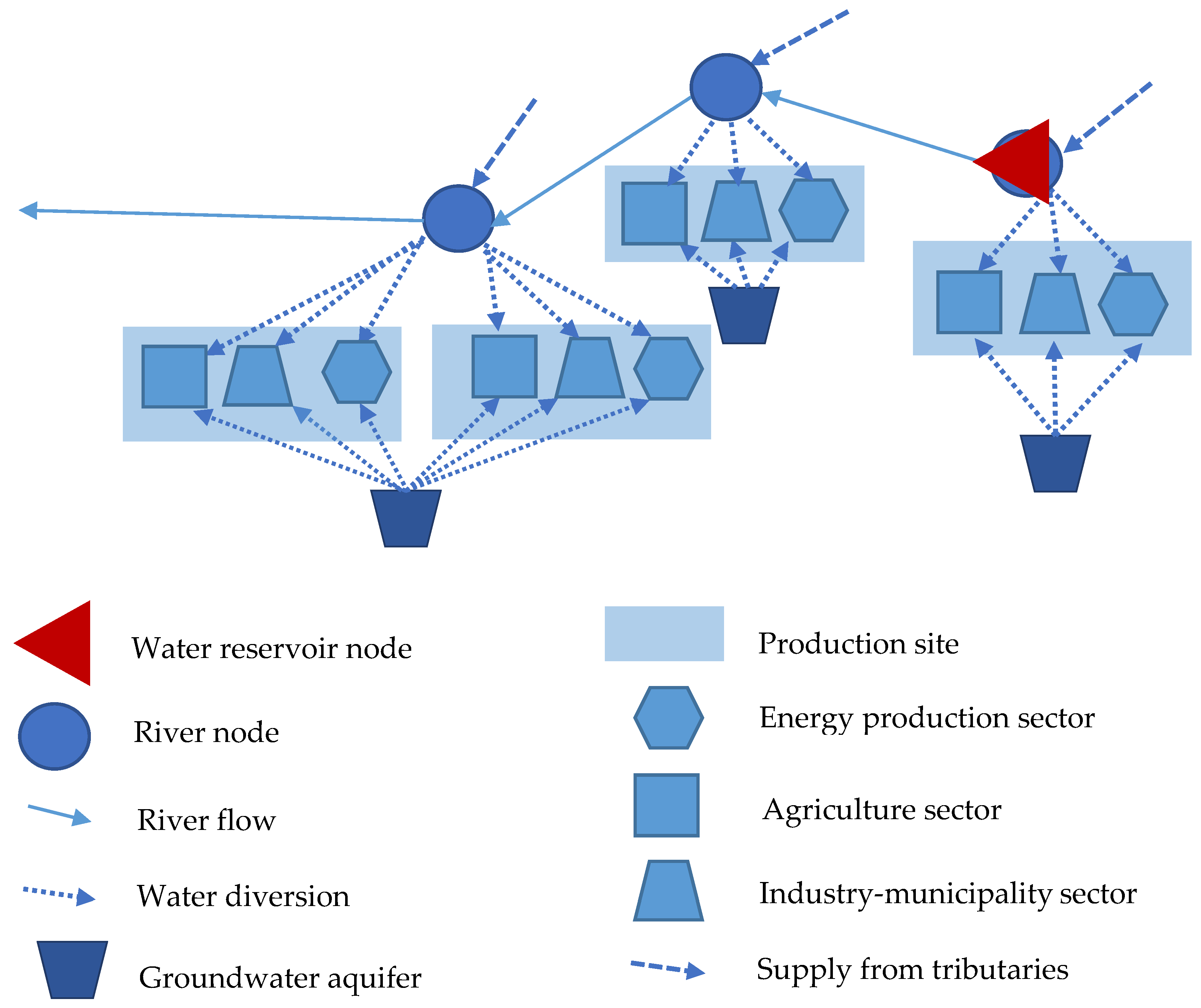
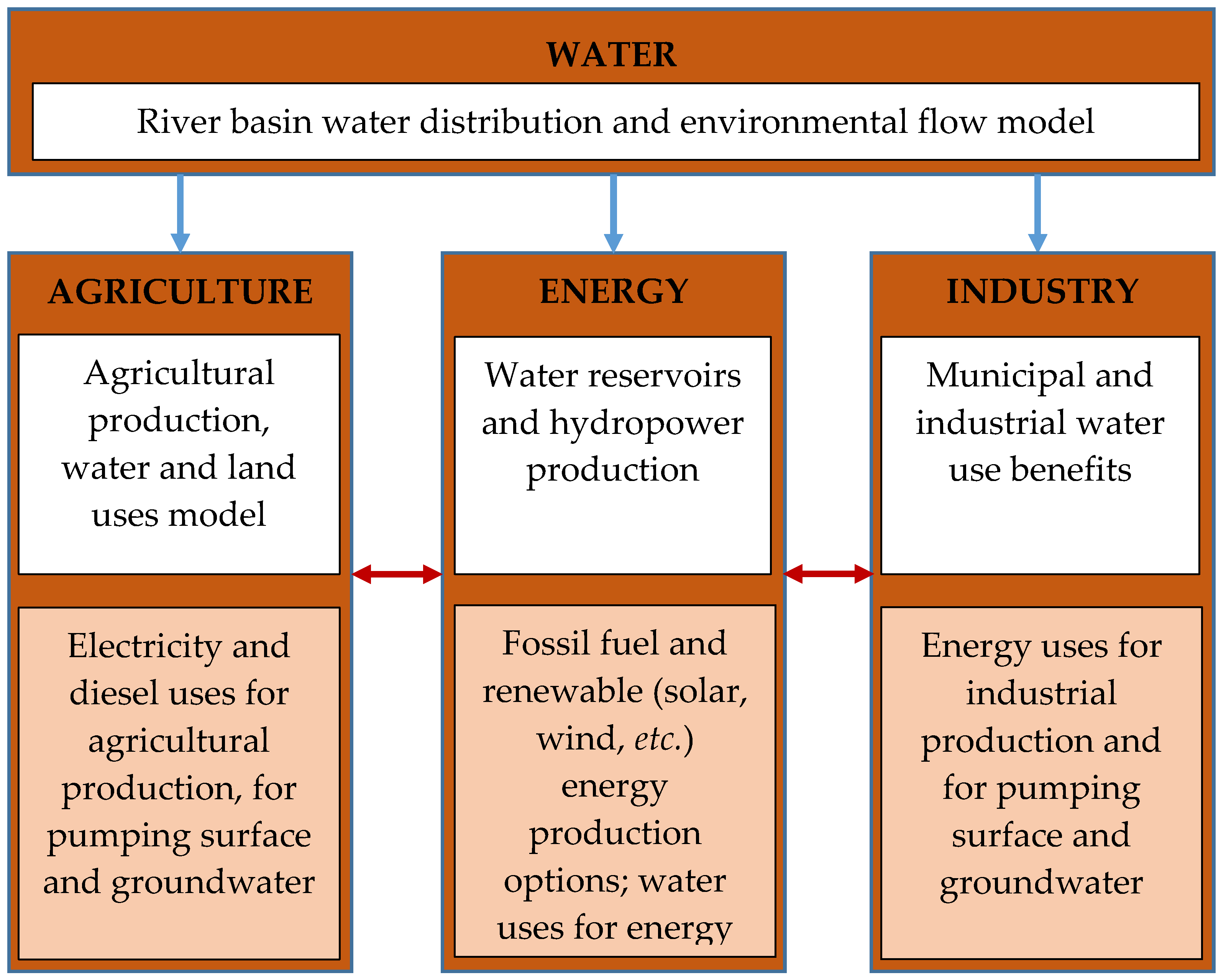
2.3. The Model Design

The core of the SEWEM is a system of equations representing a river basin system. It includes all surface and groundwater interlinkages along the river. Water uses and return flows of the production systems (the energy, agriculture, and urban and municipal sectors) are also considered. Groundwater aquifers are considered in parallel with the river nodes; thus, production sites may divert water from both surface and groundwater sources. Equations are included to relate water withdrawals and return flows with the production processes and thus to connect the core of the model with the production systems. The objective function of the SEWEM considers a maximization of the gross margins of all production sectors.

Given that all water uses and flows are interdependent and can thus effectively be traced within basin boundaries [24,34], the SEWEM is developed at a basin-scale (Scheme 1). Reservoirs and/or river nodes along a river are connected through the flow of the river. Water supply can originate from upstream tributaries as well as from local surface and groundwater sources. Three major economic sectors (or water users) are considered in the updated SEWEM: agriculture, industry-municipality, and energy production, which require water diversions from the river or reservoir nodes. Furthermore, the SEWEM foresees that a fraction of the flows delivered for production can return back to the surface and groundwater aquifers, e.g., through percolation or with drainage or wastewater flows (the so-called “return flows”; see Section 3.2 for more details of these interlinkages).

The objective function in the SEWEM maximizes the gross margins in agriculture, industry, and energy sectors across the production sites ($d$) and considers benefits from environmental flows (Scheme 2). Gross margins are calculated as the difference between revenues and production costs. Considering the focus of the study (e.g., a detailed analysis of water and energy system interlinkages), water and energy supply costs are calculated separately from the “other production costs”. The model additionally allows for an analysis of the costs of optimal water and energy use efficiency improvements and the costs of expanding energy production and water pumping stations. These aspects are included since water use efficiency improvements and a mixed use of surface and drainage water is required as a climate change adaptation measures across the arid regions of the world, while improved energy use efficiency and cleaner energy production technologies are essential as climate change mitigation measures. Agricultural outputs are calculated as the multiplication of yields to total cropped area. Crop yield reduction rates depend on seasonal water deficits, as is the case in agronomic models [35,36]. The impact of water and energy uses on the industrial value added is formulated using a Constant Elasticity of Substitution (CES) function. A linear function is considered to estimate relationships between water uses and energy outputs. Energy is used not only for production operations, but also for pumping surface water, groundwater, and drainage water. A detailed presentation of the water and energy systems is presented in Section 3.2 and Section 3.3.

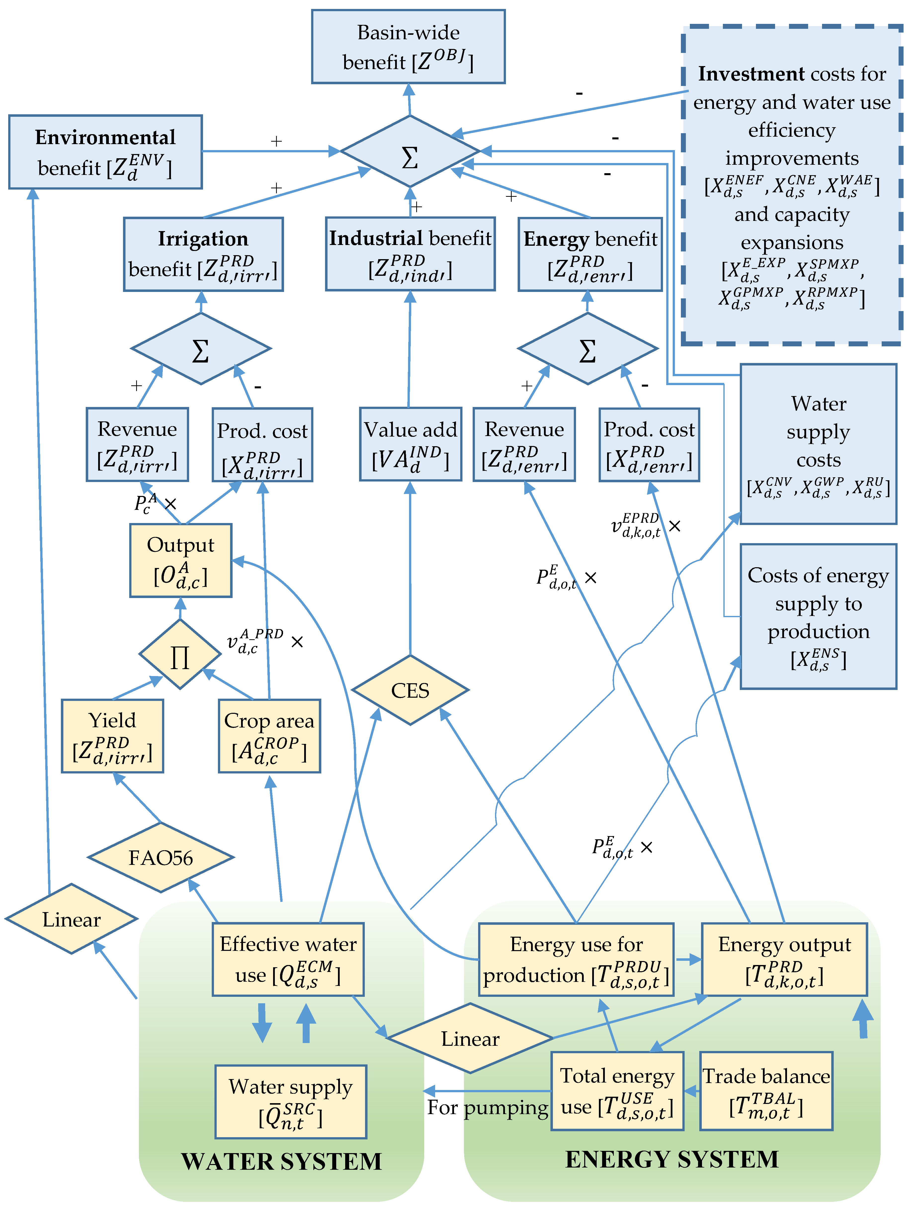
3. The Main Equations of the SEWEM

This section briefs on the key equations of the SEWEM, which represents the intra- and inter-relationships of the water, energy, and agricultural and industrial production systems. First, the objective function and economic assessments in the SEWEM are presented, which is followed by a sequential presentation of the equational constraints in the model related to water, energy, and agricultural and industrial production (food/livelihood) systems. Model variables and variable attributes (upper scripts) are written in uppercase letters, while lowercase letters are used for defining the model parameters and indices (sets) of the parameters and variables. Only key equations of the SEWEM are described in this section, but a full set of the model equations is presented in the Supplementary Materials.

3.1. Objective Function and Economic Analysis

3.1.1. The Objective Function and Sector-Specific Gross Margins

The sum of the benefits ($Z^{OBJ}$) from production (across the production sites $d$ and sectors $s$) and environmental system services is formulated as

$$Z^{OBJ}={\displaystyle \sum }_d{\displaystyle \sum }_s{Z}_{d,s}^{PRD}+{\displaystyle \sum }_n{Z}_n^{ENV}$$

(1)

where $Z_{d,s}^{PRD}$ represents the benefit in each of the three production sectors considered (energy production, industry, and agriculture) at production site $d$, $Z_n^{ENV}$ is the benefit from the environmental flow.

The sector-specific gross margins ($Z_{d,s}^{PRD}$) are calculated as the difference between economic wealth (or revenue) ($W_{d,s}^{PRD}$) and costs:

$$Z_{d,s}^{PRD}=W_{d,s}^{PRD}-X_{d,s}^{PRD}-X_{d,s}^{ENS}-X_{d,s}^{CNV}-X_{d,s}^{GWP}-X_{d,s}^{RU}-X_{d,s}^{ENEF}-X_{d,s}^{E\_EXP}-X_{d,s}^{CNE}-X_{d,s}^{WAE}-X_{d,s}^{SPMXP}-X_{d,s}^{GPMXP}-X_{d,s}^{RPMXP}$$

(2)

where

$X_{d,s}^{PRD}$ is the cost of production (other than energy and water supply costs, e.g., the sum of the costs of materials, hired labor, hired machinery, etc.);

$X_{d,s}^{ENS}$ is the cost of energy commodities delivered to the production site;

$X_{d,s}^{CNV}$ is the cost of delivering surface water to the production sectors;

$X_{d,s}^{GWP}$ is the cost of groundwater pumping used for industrial production;

$X_{d,s}^{RU}$ is the cost of the re-use of return water;

$X_{d,s}^{ENEF}$ is the cost of improving the energy use efficiency (energy use efficiency cost is a cost occurred in parallel with increased energy savings (installing energy efficient pumps, fluorescent light bulbs, etc.));

$X_{d,s}^{CNE}$ is the cost of improving the conveyance efficiency (conveyance efficiency improvement cost is a cost of saving a certain amount of water by increasing conveyance efficiency (e.g. through lining, plastic cover, etc.));

$X_{d,s}^{WAE}$ is the cost of improving the water use efficiency in the production sector $s$ (water use efficiency improvement cost is a cost induced when saving certain amount of water in a particular sector or at a production site by improving water applications (e.g., by implementing drip irrigation, subsurface irrigation, etc.));

$X_{d,s}^{E\_EXP}$ is the cost of expanding the power production capacity (expansion costs are those costs required to increase the capacity of energy production plants (e.g., by constructing additional power generation plants));

$X_{d,s}^{SPMXP}$ is the cost of expanding surface water supply (these costs occur with the expansion of water pumping stations (e.g. by constructing additional water pumping stations));

$X_{d,s}^{GPMXP}$ is the cost of expanding the groundwater pumping capacity;

$X_{d,s}^{RPMXP}$ is the cost of expanding the drainage water pumping capacity.

3.1.2. Sector-Specific Wealth (Revenues) and Production Costs

Wealth, expressed as total revenues in the energy production sector, is calculated considering energy commodity prices ($P_{d,o,t}^E$) and outputs ($T_{d,k,o,t}^{PRD}$):

$$W_{d,\prime enr\prime }^{PRD}={\displaystyle \sum }_k{\displaystyle \sum }_{o\in KOLINK}{\displaystyle \sum }_t\left(P_{d,o,t}^E{T}_{d,k,o,t}^{PRD}\right)$$

(3)

Meanwhile, the production costs in the energy sector are calculated by multiplying the average variable cost (e.g., hired labor costs, raw materials, etc.) to total energy commodity output.

Wealth in the industrial production sector ($W_{d,\prime ind\prime }^{PRD}$) is considered as equal to the industrial value added ($V{A}_d^{IND}$):

$$W_{d,\prime ind\prime }^{PRD}=V{A}_d^{IND}$$

(4)

Total revenues in the agricultural sector is calculated considering crop prices ($P_c^A$) and crop production outputs ($O_{d,c}^A$):

$$W_{d,\prime agr\prime }^{PRD}={\displaystyle \sum }_c\left(P_c^A{O}_{d,c}^A\right)$$

(5)

Crop production ($O_{d,c}^A$) is calculated as the product of crop yield and cropped area. Crop yields in turn depend on monthly water scarcity levels. Cropped areas are restricted by maximum available cropping areas along the rivers. Additional formulations that represent the relationships between water use and crop yields as well as potential irrigated area constraints are provided through Equations (S77)–(S83) in the Supplementary Materials. The production costs at the irrigation sites (here considered at the field level) consider the costs other than for water and energy supply (e.g., fertilizer, chemicals, seed, wages, etc.) and the costs for harvesting and after-harvest storage/transportation.

3.1.3. The Costs of Energy and Water Supply

The energy supply cost for production is calculated as:

$$X_{d,s}^{ENS}={\displaystyle \sum }_t\left({\displaystyle \sum }_o{P}_{d,o,t}^E T_{d,s,o,t}^{PRDU}\right)$$

(6)

where $P_{d,o,t}^E$ is the price of an energy commodity, and $T_{d,s,o,t}^{PRDU}$ is the energy use for production operations in sector $s$.

The surface water conveyance costs ($X_{d,s}^{CNV}$) are estimated as the sum of the energy costs to pump water and the costs for keeping gravitation needed for supplying water from river nodes:

$$X_{d,s}^{CNV}={\displaystyle \sum }_t\left(v_{d,s,t}^{GRV}{Q}_{d,s,t}^{GRV}+{\displaystyle \sum }_o\left(P_{d,o,t}^E T_{d,s,o,t}^{SPMP}+v_{d,s,o,t}^{SPMP}\right)Q_{d,s,o,t}^{SPMP}\right)$$

(7)

where

$v_{d,s,t}^{GRV}$ is the fixed cost per unit of surface water delivered using gravity;

$v_{d,s,o,t}^{SPMP}$ is the cost per unit of pumped surface water (hired labor, operation and maintenance, etc.);

$T_{d,s,o,t}^{SPMP}$ is the energy requirement per unit of surface water pumped;

$Q_{d,s,o,t}^{SPMP}$ is the amount of surface water pumped.

The energy costs for groundwater supply are calculated as the sum of the electricity, diesel, and other (operation and maintenance) costs for extracting groundwater for the irrigation of crops:

$$X_{d,s}^{GWP}={\displaystyle \sum }_t\left({\displaystyle \sum }_o\left(P_{d,o,t}^E T_{d,s,o,t}^{GPMP}+v_{d,o,t}^{GPMP}\right)Q_{d,s,o,t}^{GPMP}\right)$$

(8)

where

$v_{d,o,t}^{GPMP}$ is the non-energy-related cost (hired labor, operation and maintenance, etc.) of pumping per unit of pumped groundwater;

$T_{d,s,o,t}^{GPMP}$ is the amount of energy per unit of groundwater extracted through pumping;

$Q_{d,s,o,t}^{GPMP}$ is the amount of groundwater pumped.

The cost of using the return water in a demand sites is calculated as the sum of the electricity, diesel, and other (operation and maintenance) costs for extracting the groundwater:

$$X_{d,s}^{RU}={\displaystyle \sum }_t\left({\displaystyle \sum }_o\left(P_{d,o,t}^E T_{d,s,o,t}^{RPMP}+v_{d,s,o,t}^{RPMP}\right)Q_{d,s,o,t}^{RPMP}\right)$$

(9)

where

$v_{d,s,o,t}^{RPMP}$ are the non-energy-related costs (hired labor, operation and maintenance, etc.) per unit of drainage water pumped for re-use;

$T_{d,s,o,t}^{RPMP}$ is the energy requirement per unit of return water re-use;

$Q_{d,s,o,t}^{RPMP}$ is the amount of return water re-use.

Details on the calculation of different costs related to water and energy use efficiency improvements and capacity expansions of hydropower generation plants and water pumping stations are presented through Equations (S12)–(S23) in the Supplementary Materials.

3.2. Water System

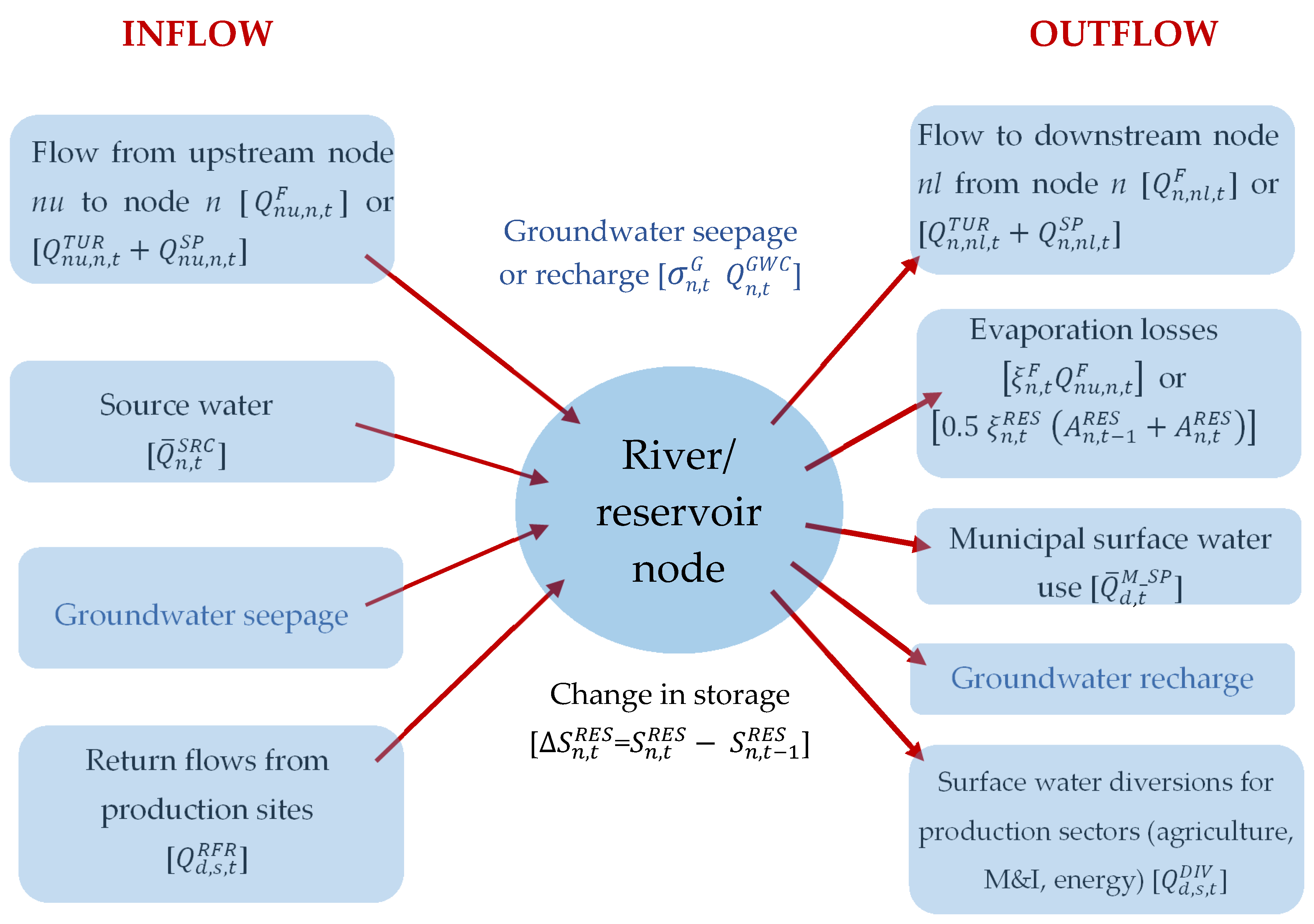
3.2.1. Water Balance at River Node (Reservoir)

The water balance at the river and reservoir nodes in the SEWEM is based on the equality of all inflows to the node with all outflows from the node (Scheme 3). Water inflows are assumed to stem from upstream nodes, from surface water supply sources, from groundwater seepage to the river, and from return flows. Water outflows are those to downstream nodes, to production sites (e.g., irrigation fields, energy, and municipal-industrial sites), as evaporative losses, and losses to groundwater aquifers. In case of the reservoir nodes, changes in water storage are added.

Following this definition, the water balance in river and reservoir nodes can be formulated as:

$$\begin{gathered} {\overline{Q}}_{n,t}^{INF}+\left(1-{\xi }_{n,t}^F\right)\left[{\displaystyle \sum }_{nu\in NNLINK}\left(1-{\sigma }_{nu}^{RES}\right)Q_{nu,n,t}^F+{\displaystyle \sum }_{nu\in NNLINK}{\sigma }_{nu}^{RES}\left(Q_{nu,n,t}^{TUR}+Q_{nu,n,t}^{SP}\right)\right] \\ +{\displaystyle \sum }_s{\displaystyle \sum }_{d\in DNLINK}{Q}_{d,s,t}^{RFR} \\ ={\sigma }_n^{RES}\left[\Delta S_{n,t}^{RES}+\frac{{\xi }_{n,t}^{RES}}{2}\left(A_{n,t-1}^{RES}+A_{n,t}^{RES}\right)\right]+\left(1-{\sigma }_n^{RES}\right){\displaystyle \sum }_{nl\in NNLINK}{Q}_{n,nl,t}^F \\ +{\sigma }_n^{RES}{\displaystyle \sum }_{nl\in NNLINK}\left(Q_{n,nl,t}^{TUR}+Q_{n,nl,t}^{SP}\right)+{\displaystyle \sum }_{d\in NDLINK}\left({\displaystyle \sum }_s{Q}_{d,s,t}^{DIV}+{\overline{Q}}_{n,t}^{M\_SP}\right)+{\sigma }_{n,t}^G{Q}_{n,t}^{GWC} \end{gathered}$$

(10)

where

${\overline{Q}}_{n,t}^{INF}$ is the flow from the source node (runoff) at time $t$;

${\xi }_{n,t}^F$is the rate (in %) of evaporative loss of flows to node $n$;

$Q_{nu,n,t}^F$ is the river flow from the upstream node $nu$ to node $n$ (given a link $\left(nu,n\right)\in NNLINK$ between these nodes);

${\sigma }_n^{RES}$is a binary parameter that equals to 1 if the node $n$ is a reservoir, or 0 otherwise;

$Q_{nu,n,t}^{TUR}$ and $Q_{nu,n,t}^{SP}$ are flows through the turbines and spillways flowing to node $n$ from the upstream reservoir node $nu$, respectively;

$Q_{n,s,t}^{RFR}$is the return flow to the river node $n$, e.g., from irrigated production, of from municipal and industrial, and energy production $s$;

$Q_{n,t}^{GWC}$ is the aquifer recharge with water stemming from the river node $n$;

$S_{n,t}^{RES}$ is reservoir storage volume at node n;

${\xi }_{n,t}^{RES}$ is the evaporative loss (in depth per unit time) from the surface of the reservoir;

$A_{n,t}^{RES}$ is the surface area of the reservoir;

$Q_{d,s,t}^{DIV}$ is the surface water withdrawal from river node to the production site $d$ and sector $s$ (e.g., irrigation, municipal and industrial, power production sector);

${\sigma }_{n,t}^G$ is a binary parameter that takes a value of either −1, 0, or 1 depending on the direction of the flow in-between the groundwater aquifer and the river system, which thus may vary over time and in space (if ${\sigma }_{n,t}^G=1$, then groundwater recharge occurs; if ${\sigma }_{n,t}^G=-1$, then groundwater seepage to the river node occurs; ${\sigma }_{n,t}^G=0$ indicates no water flow between river node and groundwater aquifer);

${\overline{Q}}_{d,t}^{M\_SP}$ is the surface water use by municipality (Note: municipal water use is assumed to be fixed and separate from industrial water use since residential water use is often prioritized in water allocation decisions).

Additional constraints related to the capacity or maximum water level at the reservoirs, and the relationships between reservoir head and volume are presented through Equations (S25)–(S28) in the Supplementary Materials.

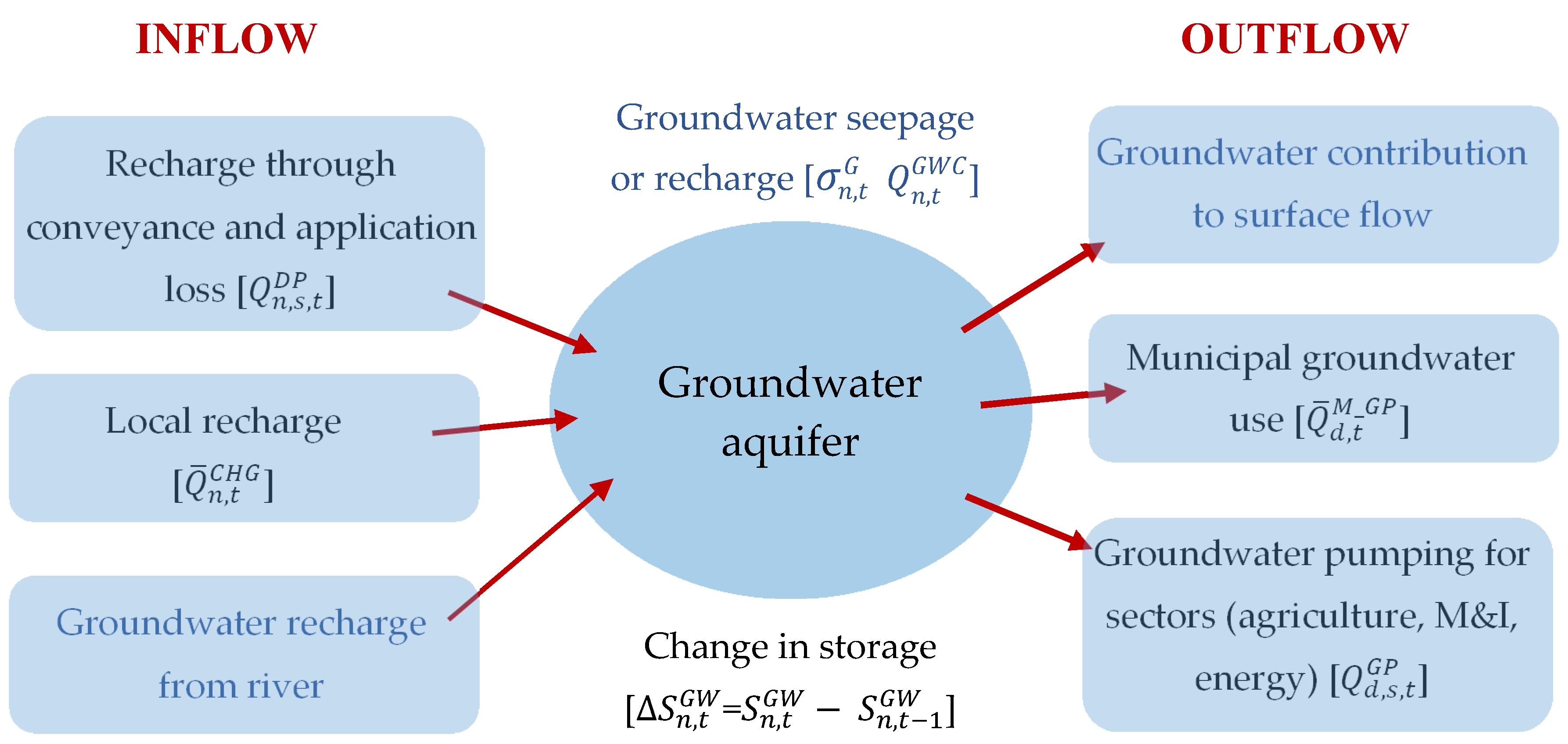
3.2.2. Groundwater Balance

Groundwater aquifers are considered in parallel with each river node. The production sites connected to a particular river node can also use water from the related groundwater aquifer. Like the surface water balance in the nodes, the groundwater balance considers an equity of total inflows and outflows plus water volume changes in the aquifer (Scheme 4). Groundwater volume changes can be provoked by percolation from production sites, fields, and irrigation canals, groundwater use and water seepage to (and from) the river.

Following this description, the water balance relationship in groundwater aquifers is:

$${\overline{Q}}_{n,t}^{CHG}+{\sigma }_{n,t}^G{Q}_{n,t}^{GWC}+{\displaystyle \sum }_{d\in NDLINK}{\displaystyle \sum }_s{Q}_{d,s,t}^{DP}=\Delta S_{n,t}^{GW}+{\displaystyle \sum }_{d\in NDLINK}\left({\displaystyle \sum }_s{Q}_{d,s,t}^{GP}+{\overline{Q}}_{d,t}^{M\_GP}\right)$$

(11)

where

${\overline{Q}}_{n,t}^{CHG}$ is the monthly groundwater aquifer charge;

$Q_{d,s,t}^{DP}$ is the deep percolation (during conveyance and water application (use) at production sites);

$S_{n,t}^{GW}$ is the water volume in the groundwater aquifer, which is parallel to river node $n$;

$Q_{d,s,t}^{GP}$ is the groundwater use by sector $s$ at node $n$;

${\overline{Q}}_{d,t}^{M\_GP}$ is the groundwater use by the municipal sector.

Additional constraints that represent for instance maximum groundwater aquifer heads and factors that determine groundwater seepage and volume changes are provided through Equations (S30)–(S32) in the Supplementary Materials.

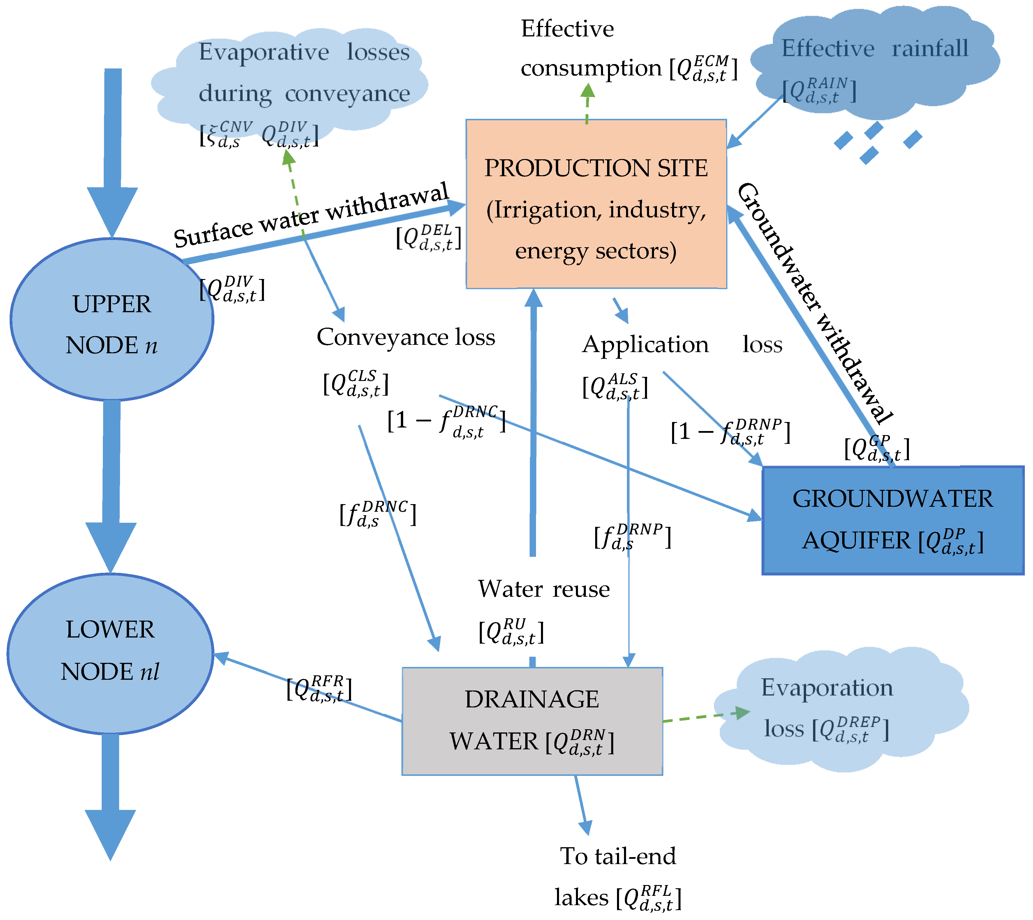
3.2.3. Water Supply and Use Relationships at Production Sites

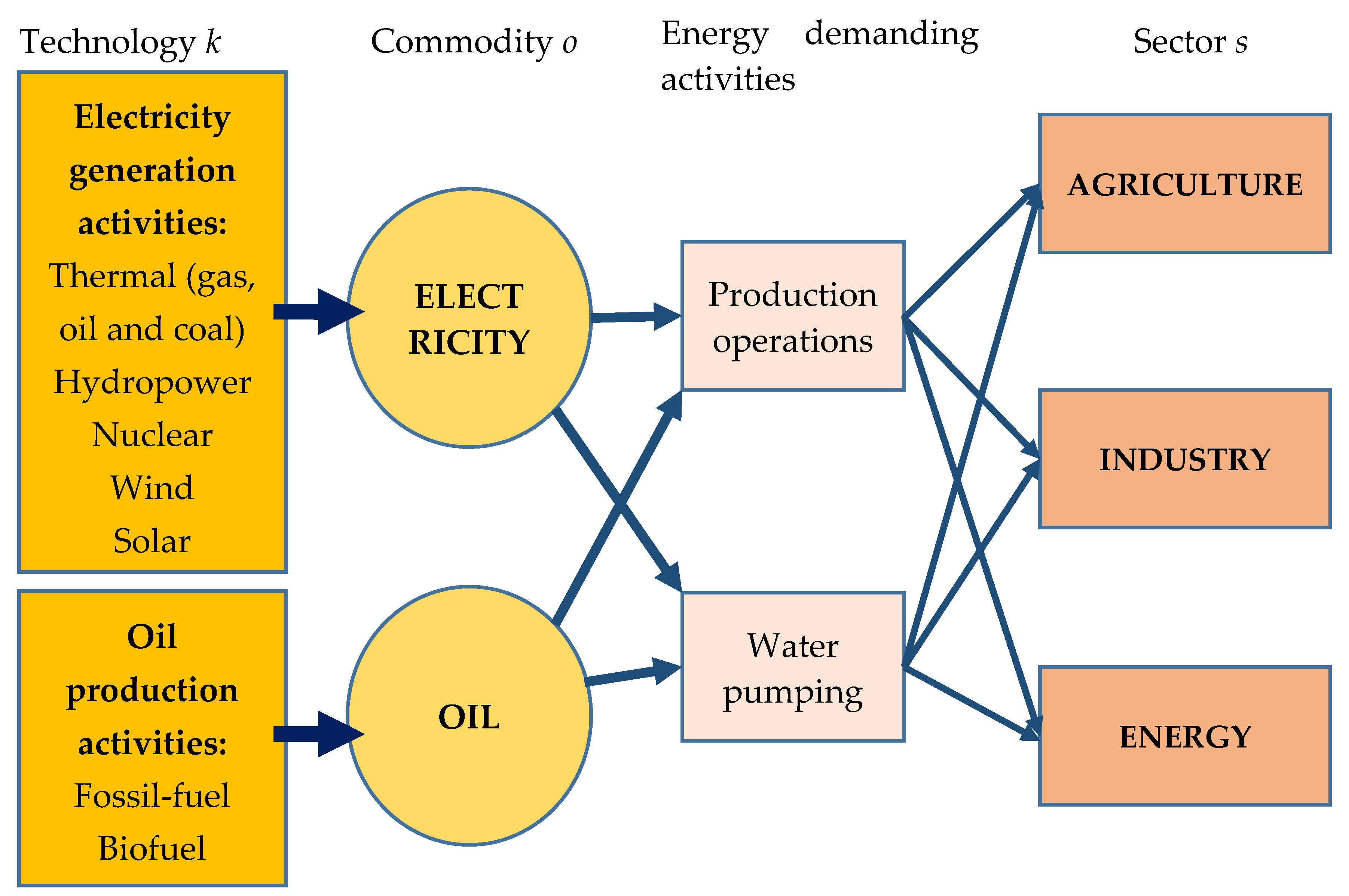
The water balance at any production node considers water conveyance, effective consumption, deep percolation, and return-flow relationships (Scheme 5). Surface water diverted for production is partially lost during conveyance owing to non-productive evaporation losses, and seepage to the groundwater aquifers and drainage systems. Water use for any production site originates from the surface water sources, groundwater pumping, or reuse of drainage water. In the case of agriculture, for instance, additional water to crops is assumed to become available through precipitation. According to the water balance relationships, only a part of the water delivered to a production site is effectively used, while the remaining water is lost. The water lost either joins the groundwater aquifer or ends up as drainage water. Return flows (e.g., drainage waters) are split among the river, non-productive evaporation losses, and flows into the sinks located at the ends of drainage canals.

Total water delivered to the production site from river nodes ($Q_{d,s,t}^{DEL}$) was estimated by considering conveyance efficiency ($E_{d,s}^{CNV}$), evaporation losses (${\xi }_{d,s}^{CNV}$), and water withdrawals ($Q_{d,s,t}^{DIV}$) for the production purposes:

$$Q_{d,s,t}^{DEL}=\left(1-{\xi }_{d,s}^{CNV}\right)Q_{d,s,t}^{DIV}{E}_{d,s}^{CNV}$$

(12)

Total water use or application at a production site ($Q_{d,s,t}^{USE}$) originates from surface ($Q_{d,s,t}^{DEL}$), aquifer ($Q_{d,s,t}^{GP}$), and drainage water ($Q_{d,s,t}^{RU}$) sources:

$$Q_{d,s,t}^{USE}=Q_{d,s,t}^{DEL}+Q_{d,s,t}^{GP}+Q_{d,s,t}^{RU}$$

(13)

The applied water ($Q_{d,s,t}^{USE}$) is either effectively consumed or lost through evaporation or return flows:

$$Q_{d,s,t}^{USE}=\left(Q_{d,s,t}^{ECM}-Q_{d,s,t}^{RAIN}\right)+Q_{d,s,t}^{ALS}$$

(14)

where $Q_{d,s,t}^{RU}$ is the re-use of the return flow, $Q_{d,s,t}^{RAIN}$ is the effective rainfall (for crops only), $Q_{d,s,t}^{ECM}$ is the effective water consumption, and $Q_{d,s,t}^{ALS}$ is the loss of water during application.

Water losses during conveyance are estimated as

$$Q_{d,s,t}^{CLS}=\left(1-{\xi }_{d,s}^{CNV}\right)Q_{d,s,t}^{DIV}\left(1-E_{d,s}^{CNV}\right)$$

(15)

where ${\xi }_{d,s}^{CNV}$ is a coefficient indicating evaporation losses.

Part of the losses during conveyance and water applications joins the drainage systems. Thus, the drainage waters ($Q_{d,s,t}^{DRN}$) are composed of shares of water losses during conveyance and water applications:

$$Q_{d,s,t}^{DRN}=Q_{d,s,t}^{CLS}{f}_{d,s}^{DRNC}+Q_{d,s,t}^{ALS}{f}_{d,s}^{DRNP}$$

(16)

$f_{d,s}^{DRNP}$ and $f_{d,s}^{DRNC}$ are fractions of water losses during water applications and conveyance, respectively, and end up as drainage water.

Part of the losses during conveyance and water applications seeps into the groundwater aquifer ($Q_{d,s,t}^{DP}$) through percolation:

$$Q_{d,s,t}^{DP}=Q_{d,s,t}^{CLS}\left(1-f_{d,s}^{DRNC}\right)+Q_{d,s,t}^{ALS}\left(1-f_{d,s}^{DRNP}\right)$$

(17)

The return flow to the river from any production site and sector ($Q_{d,s,t}^{RFR}$) is calculated as the remaining drainage water after subtracting the amounts of flows to the tail-end depressions, losses to evaporation, and re-uses:

$$Q_{d,s,t}^{RFR}\le Q_{d,s,t}^{DRN}-Q_{d,s,t}^{RFL}-Q_{d,s,t}^{DREP}-Q_{d,s,t}^{RU}$$

(18)

where $Q_{d,s,t}^{RU}$ is the amount of water re-use, $Q_{d,s,t}^{RFL}$ is the flow to the tail-end sinks, and $Q_{d,s,t}^{DREP}$ is the evaporative losses from the drainage systems calculated as a fixed ratio of drainage waters.

More detailed representations of water distribution within the sectors (e.g., water use by crops, energy generation activities, water pumping using electricity or liquid fuel, etc.) are given through Equations (S40)–(S62) in the Supplementary Material.

3.3. Energy System

Energy generation is assumed to be based on the different energy production technologies, while the energy use is considered for different production activities (Scheme 6).

The energy supply to the regional market $m$ ($T_{m,o,t}^{SUP}$) is the sum of energy production ($T_{d,k,o,t}^{PRD}$) by different technologies $k$ at each of the production site ($d$) that is connected to this market ($n\in MDLINK$):

$$T_{m,o,t}^{SUP}={\displaystyle \sum }_{d\in MDLINK}{\displaystyle \sum }_{k\in KOLINK}{T}_{d,k,o,t}^{PRD}$$

(19)

The total energy (generated by electricity or diesel) supplied to the energy market $m$ is assumed to be distributed among the production sectors $s$ connected to the regional energy market ($\left(m,d\right)\in MDLINK$):

$$T_{m,o,t}^{SUP}={\overline{T}}_{m,o,t}^{TBAL}+{\displaystyle \sum }_{d\in MDLINK}{\displaystyle \sum }_s\left[\left(1+r_{d,s,o,t}^{ELOSS}\right)\left(T_{d,s,o,t}^{USE}+{\overline{T}}_{d,o,t}^{M\_USE}\right)\right]$$

(20)

where

$T_{d,s,o,t}^{USE}$ is the energy use (both for production operations and for pumping water from surface, ground, and drainage water sources) by the production sectors considered (agriculture, energy, and industry);

${\overline{T}}_{d,o,t}^{M\_USE}$ is the energy use by the municipal sector (separate from the energy use by the industry and considered as fixed assuming a priority of the municipal sector in energy allocation decisions);

${\overline{T}}_{d,o,t}^{TBAL}$ is the energy trade balance. This takes a positive value in case energy is exported out of the regional market, but a negative value when energy is imported to the regional market);

$r_{d,s,o,t}^{ELOSS}$ is a discount coefficient that takes into account the energy losses during transportation (transmission) and distribution.

The total energy demand by production sector $s$ ($T_{d,s,o,t}^{USE}$) in period $t$ is accumulated as the sum of the energy uses for pumping surface water, groundwater, re-use of return flow, and running production activities ($T_{d,s,o,t}^{PRDU}$):

$$T_{d,s,o,t}^{USE}=T_{d,s,o}^{SPMP}{Q}_{d,s,o,t}^{SPMP}+T_{d,s,o,t}^{GPMP}{Q}_{d,s,o,t}^{GPM}+T_{d,s,o}^{RPMP}{Q}_{d,s,o,t}^{RPMP}+T_{d,s,o,t}^{PRDU}$$

(21)

where

$T_{d,s,o}^{SPMP}$ is the energy demand to deliver one unit of surface water to an irrigation site;

$T_{d,s,o,t}^{GPMP}$ is the energy demand to pump one unit of groundwater (varies depending on groundwater depth);

$T_{d,s,o}^{RPMP}$ is the energy requirement to pump one unit of water out of the drainage-collector system.

A full set of equations that represent the energy generation and use relationships in the model are presented through Equations (S66)–(S74) in the Supplementary Material.

4. Implementation of the Model

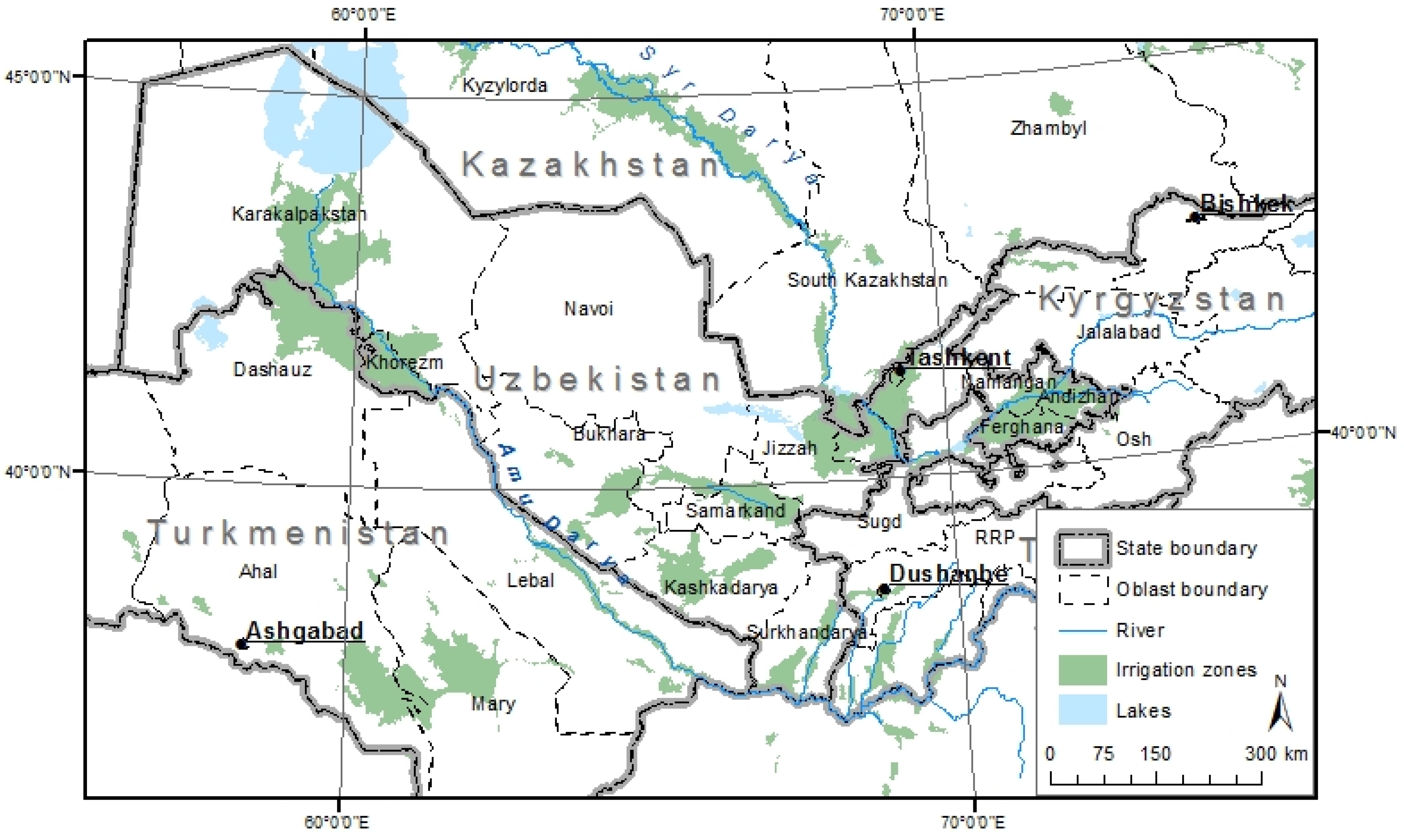
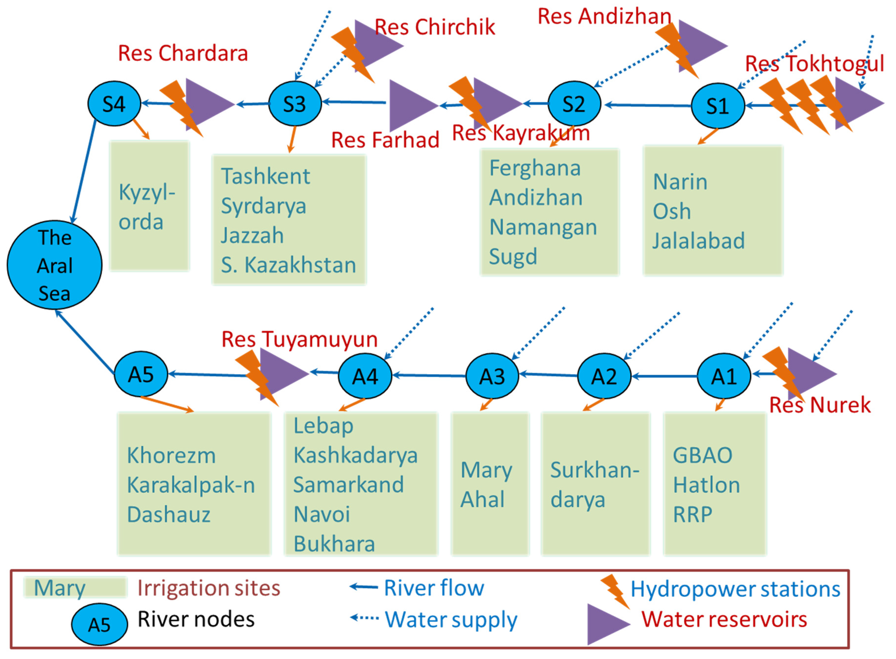
4.1. Description of the Study Area and River Network Scheme

Following the completion of the SEWEM, it was parametrized for the case of the Aral Sea Basin (ASB) in Central Asia and next implemented to show the potential impact of energy constraints on water and land allocation decisions on the scale of a basin. Earlier versions of the model that included a detailed representation of river basin water allocation, agricultural production, hydropower generation, surface and groundwater aquifer relationships, as well as options to improve water use efficiency, had been used to assess the economic and water saving effects of irrigation technologies as well as to analyze the trade-offs between irrigation and hydropower development [17,27]. Therefore, detailed discussions on water and land uses in the basin are presented elsewhere [17,27], while the focus here is on the water, energy, and irrigation system interlinkages in the ASB.

Despite abundantly available water resources at basin scale, all of Central Asia is saddled with a water problem. Moreover, due to the predicted growth in population, irrigation expansion, and industrial development, the pressure on these water resources is predicted to increase, which in turn will challenge managers and users of water alike even more than today. To cope effectively with the expected water challenges, improved water resources planning and management is a prime pathway to cope with the increased water demands in the most efficient way while, in addition, aiming at improving water productivity across all sectors of the economy. Water productivity can be improved through the adoption of irrigation technologies such as drip or sprinkler irrigation, or through a re-allocation or diversification of the water supply, for example by changing pumping capacities along the rivers. Furthermore, additional energy production may be needed to satisfy the additional energy demands linked to increased irrigation water withdrawals, which may in turn require additional water, thus challenging an irrigation expansion. Since such means and options require substantial amounts of energy, the introduction, use, or spread of innovations has consequences for both the energy demand and supply systems.

The majority of the ASB coincides with the territories of the five Central Asian countries—Uzbekistan, Kazakhstan, Turkmenistan, Tajikistan, and Kyrgyzstan (Figure 2) [37,38]. More than 60% of the population in the basin lives in rural areas and their livelihood directly depends on irrigation and thus water availability from the rivers—the Amu Darya and Syr Darya [38]. For more than three millennia, waters from these two key rivers have been vital for the development and blossoming of the ancient cultures in the region, which went hand in hand with agricultural development. Water from both rivers originates from the mountain ranges of the Pamirs and Tien-Shan located in the upstream countries of Kyrgyzstan, Tajikistan, and Afghanistan. During the Soviet era (1924–1991), and particularly since the late 1950s, water from both rivers was extracted excessively to supply the immense irrigation systems. Cotton production was particularly extended to gain cotton self-sufficiency in the former Soviet Union both through the expansion of irrigated croplands and at the expense of replacing staple crops. Consequently, cotton covered more than half of the irrigated croplands in Uzbekistan in the pre-independence period. Though cotton production was slightly reduced following independence, it has been maintained because of its importance for generating hard currency revenues [39,40]. For improving food and income security and for boosting sustainable economic growth, croplands have also been passed over to households to grow fruits, vegetables, and staple crops. As a result, irrigated winter wheat production grew rapidly in importance after independence in 1991 to gain grain self-sufficiency in Uzbekistan, Turkmenistan, and Tajikistan [41]. Thus, the size of the irrigated croplands has been extended to more than 7 million ha (Mha) during the last five to six decades [42]. Particularly, the construction of the Amu-Bukhara (Uzbekistan), Karshi (Uzbekistan), and Karakum (Turkmenistan) canals, which have been equipped with large pumping stations to lift water to the massive cropping areas in Bukhara, Kashkadarya, and Mary provinces, evidences the extent of the irrigation development in a very short time [43]. Yet, the expansion of irrigation has resulted in increased irrigation water withdrawals also, which in the end has substantially contributed to the desiccation of the Aral Sea [37,39,44,45,46].

Although roughly 85% of the total surface water resources in the region are formed within the upstream countries Kyrgyzstan, Tajikistan and Afghanistan, the chief water users are the downstream nations Uzbekistan, Turkmenistan, and Kazakhstan. During the Soviet Union era, this artificially created ill-balance in “production” and consumption of water was initially well-managed. The centrally planned system of water quotas regulated water allocation among the five Central Asian republics with the overall aim of providing irrigation water to downstream regions in the summer for maximizing crop production. Meanwhile, in exchange for water, the energy-scarce upstream republics (Kyrgyzstan and Tajikistan) received fossil fuels (coal and gas) to generate electricity and heat at heavily subsidized prices. Irrigation practices relied on surface water resources, as evidenced by the share of groundwater sources to satisfy crop water demand, which is limited to 3%–4% of total water withdrawals only [47]. The surface water withdrawals largely depend on pumping that requires substantial amounts of energy [48]. These energy demands for pumping were partially met through excess hydropower generation by the upstream countries during summer [49]. Yet, following independence from the Soviet Union, this centrally managed “water-energy-food/livelihood nexus” collapsed. Currently, large quantities of water are released by the upstream countries during winter for generating their highly needed electric power to satisfy their own heating demands during this peak season [50,51]. However, while doing so, less water remains to satisfy the water demand in the downstream countries, particularly during the summer irrigation seasons.

Due to the initial set up and interdependencies, the highest economic gains can be achieved only through re-vitalizing the previous intensive cooperation among the countries in Central Asia, while aiming at a basin-wide optimization of water allocation as frequently suggested [52]. Since this is not the case anymore, an integrated assessment of water and energy allocations could revamp the urge to apply optimal levels of water demand for improved food and energy security. Climate-change-induced reductions in river runoff under conditions of increasing demands for water due to a growing population and industrial growth requires additional sources of water supply. Given the limited use of non-surface water (currently groundwater uses are ca. 3%–4% of total water uses), an increased use of groundwater and drainage water re-uses could ease the recurrently occurring water stresses [48]. However, given the heavy dependence of irrigation water supply, especially groundwater extraction for irrigation, on energy availability, and the limitedness of energy supply due to a sky-rocketing of energy prices following independence, a consideration of energy requirement restrictions and the possibilities of expanding alternative energy production options may provide an additional insight on economically relevant levels of surface and groundwater uses and land allocations. Although many advocate better planning based on an integrated assessment of water, energy, and food/livelihood systems [52], real progress has been modest because only the hydrological and economical aspects had been taken into account in previous hydro-economic models, while energy aspects had usually been ignored. The application of the SEWEM addresses these deficiencies.

The river network scheme of SEWEM applied to the case of the ASB considered production activities across the provinces through which the two main rivers in Central Asia—the Amu Darya and Syr Darya—flow (Scheme 7). Furthermore, only large hydropower production plants and large reservoirs have been included. Water supplies originated mainly from the upstream river reaches, and only partially from the mid-stream reaches. Driven by data limitations and the large, spatial-scale of the analysis intended, the river basin scheme of the model considered the aggregated river nodes and production sites only.

4.2. Model Database, Assumptions, Scenarios, and Solutions

The database of the SEWEM could be composed after tapping multiple primary and secondary sources (

Table 1. Main sources of the SEWEM database.

#	Data Description	Source
1	Water uses by sectors, irrigated land, agricultural yields, agricultural production costs and benefits	SIC-ICWC [53,54], EC-TACIS [55]
2	Costs for improving water application and conveyance efficiencies	Cai [56], SIC-ICWC [57]
3	Seasonal crop coefficients for estimating relationships between monthly water uses and crop yield	Cai [56], Schieder [58]
4	Parameters for depicting the relationships between reservoir head and volume, hydropower production outputs and costs	SIC-ICWC [59], EC-IFAS [60]
5	Costs, benefits, and development potentials of alternative energy production	CER [61], World Bank [62]

). The information on land and water uses, water supplies, agricultural yields and outputs, and agricultural production benefits and costs are based on reports prepared by SIC-ICWC [53,54] and EC-TACIS [55]. Crop prices have been additionally cross-checked and improved based on market survey data by the ZEF/UNESCO project. The costs for improving the water application and conveyance efficiencies are based on studies conducted by Cai [56] and SIC-ICWC [57]. The seasonal crop coefficients used for estimating the relationships between water use and crop yield are based on Cai [56] and Schieder [58]. Hydropower production and the parameters characterizing the relationships between reservoir head and volume are based on various modeling studies conducted in the region [59,60]. Costs, benefits, as well as development potentials of alternative energy production across the basin have been reported by CER [61] and the World Bank [62]. When data was assessed as inadequate or insufficient for model calibration, simplified versions of the energy and agricultural commodity demand functions had been considered assuming an absolute price elasticity of demand, e.g., by assuming fixed energy and agricultural commodity prices. A more detailed presentation of data and sources can be found in Bekchanov [38]. The SEWEM model is calibrated considering “normal water supply,” which is assumed to be an average of the supplies observed between 1980 and 2000. Based on data availability, all economic costs and benefits are considered at price levels of 2005.

Since the SEWEM is based on an optimization approach, a full cooperation among the riparian countries and provinces in the basin is assumed. Hence, during the test-case, the findings of the optimization run mirror the case when all five countries in Central Asia would cooperate with each other to gain the highest, basin-wide gains and while assuming that these benefits are shared fairly among these countries.

To underscore the impact on the sectoral gross margins as well as the spatial allocation of water and land resources when considering the energy sub-system, two runs, called hereafter “experiments,” were prepared. In the first experiment, the energy component was excluded (except for hydropower production) from the model by deactivating the Equations (20)–(22) that reflect energy production and consumptions. Thus, in Equations (7)–（10) that relate to energy and water supply costs, several variables such as energy prices ($P_{d,o,t}^E$), energy uses by sectors ($T_{d,s,o,t}^{PRDU}$), and energy requirements per unit of surface water supply ($T_{d,s,o,t}^{SPMP}$), groundwater supply ($T_{d,s,o,t}^{GPMP}$), and drainage water pumping ($T_{d,s,o,t}^{RPMP}$) were disconnected from the energy balance equations and used only for calculating the energy and water supply costs. In contrast, in the second experiment, all equations related to energy production and use had been activated and became hence part of the analyses. Additionally, activated were those routines addressing energy uses for pumping and production processes that are constrained by energy availability according to the equations of the energy block as described in Section 3.3. The differences between the findings of both experiments thus are an indication of contrasting optimal water use and benefits when additionally considering an alternative, non-hydropower-based energy production system and the energy requirement constraints for irrigation water supply. The SEWEM is coded in GAMS and solved using the Conopt3 Solver.

4.3. Model Simulation Results

To show the importance of an inclusion of those constraints related to energy production and consumption on surface and groundwater use decisions, the related modeling outcomes are presented across all the sub-regions (here provinces) of the ASB (

Table 2. Optimal levels of groundwater (GW) and surface water (SW) withdrawals without (Experiment 1) and while (Experiment 2) considering the energy production and consumption sub-module. Provinces underlined are in Tajikistan, those underlined and in italics are in Kyrgyzstan, and those in italics are in Turkmenistan. Provinces in italics and bold are in Kazakhstan, and those in a normal typeface (i.e., not underlined, in italics, or bold) are in Uzbekistan.

Basin	Provinces	Exp1: Without Energy Component			Exp2: With Energy Component			Difference between Exp1 and Exp2
		GW (million m3)	SW (million m3)		GW (million m3)	SW (million m3)		GW (%)	SW (%)
Amu Darya	GBAO	50	314		19	370		−63	18
	Khatlon	410	1722		412	1933		0	12
	RRP	0	893		0	893		n/a	0
	Surkhandarya	292	6711		292	6443		0	−4
	Mary	0	8730		0	7559		n/a	−13
	Ahal	0	6100		0	4047		n/a	−34
	Lebap	0	5757		0	5757		n/a	0
	Kashkadarya	508	7836		317	4729		−38	−40
	Samarkand	457	8594		171	8946		−63	4
	Navoi	131	3264		49	3262		−62	0
	Bukhara	199	4881		199	3056		0	−37
	Khorezm	0	3719		0	3788		n/a	2
	Karakalpakstan	0	7011		0	6976		n/a	0
	Dashauz	0	7079		0	7103		n/a	0
Syr Darya	Narin	36	286		35	288		−1	1
	Osh	53	497		50	499		−5	0
	Jalalabad	39	428		38	428		−3	0
	Ferghana	284	4390		273	4408		−4	0
	Andizhan	150	2874		150	2874		0	0
	Namangan	251	3693		224	3682		−11	0
	Sugd	183	1757		168	1754		−8	0
	Tashkent	485	4283		485	4286		0	0
	Syrdarya	159	4160		135	4187		−15	1
	Jizzah	176	3642		182	2775		3	−24
	S.Kazakhstan	0	4351		0	4542		n/a	4
	Kyzylorda	0	2003		0	2003		n/a	0
	Total:	3865	104,975		3199	96,589		−17	−8

Note: GBAO—Gorno-Badakhshan Autonomous Oblast; RRP—Regions of the republican subordination.

). For instance, several locations showed a high sensitivity of surface and groundwater pumping when considering the imposed energy use constraints, particularly in the mountainous provinces such as Gorno-Badakhshan Autonomous Oblast (GBAO) in Tajikistan, or the Samarkand and Navoi provinces in Uzbekistan. Consequently, the size of the irrigated areas in such locations would reduce by more than 60% when considering such energy use restrictions. Moreover, in Bukhara and Kashkadarya provinces (both Uzbekistan), irrigation heavily depends on the extraction of massive amounts of surface water through pumping; hence, optimal surface water use would be reduced by almost 40% when energy use restrictions are considered. In the Mary and Ahal provinces of Turkmenistan, irrigation water losses used to be enormous, since irrigated agriculture is practiced on sandy soils. Consequently, irrigation water delivery and distribution requires a substantial amount of energy use per unit of consumed water. Therefore, surface water uses in these regions are likely to decrease (e.g., by 13% and 34% respectively) when facing energy use restrictions. On the other hand, reductions in basin-wide irrigation benefits caused by an absolute reduction in water use in some provinces (e.g., Samarkand, Navoi, Mary, Ahal) were compensated for in part by an increased surface water use in other provinces with higher marginal water use benefits such as in GBAO and Khatlon (Tajikistan) by 18% and 12%, respectively. Because of the energy use constraints introduced in the model, optimal levels of groundwater and surface water uses basin-wide would decrease by 17% and 8%, respectively. The differences in results imply possible overestimations of optimal water uses in most hydro-economic models when energy requirements for water supply and energy supply restrictions are ignored.

Changes in irrigation-driven benefits would follow the pattern of water use changes across the provinces (

Table 3. Optimal levels of irrigation benefits without (Experiment 1) and with (Experiment 2) considering the energy production and consumption sub-module. Provinces underlined are in Tajikistan, those underlined and in italics are in Kyrgyzstan, those in italics are in Turkmenistan, those in italics and bold are in Kazakhstan, and those in a normal typeface (i.e., not underlined, in italics, or bold) are in Uzbekistan.

Basin	Provinces	Irrigation Benefits (million USD)			Difference between Exp1 and Exp2 (%)
		Exp1: Without Energy Constraints	Exp2: With Energy Constraints
Amu Darya	GBAO	35	35		1
	Khatlon	176	184		4
	RRP	59	59		1
	Surkhandarya	126	131		4
	Mary	233	219		−6
	Ahal	76	66		−13
	Lebap	142	143		1
	Kashkadarya	377	341		−9
	Samarkand	198	202		2
	Navoi	47	43		−8
	Bukhara	83	60		−28
	Khorezm	107	106		−1
	Karakalpakstan	190	187		−1
	Dashauz	208	208		0
Syr Darya	Narin	12	13		6
	Osh	52	53		2
	Jalalabad	56	57		2
	Ferghana	117	121		4
	Andizhan	162	164		1
	Namangan	161	170		5
	Sugd	80	86		7
	Tashkent	177	181		2
	Syrdarya	174	178		2
	Jizzah	80	66		−17
	S.Kazakhstan	177	183		3
	Kyzylorda	73	73		−1
	Total:	3378	3328		−1

Note: GBAO—Gorno-Badakhshan Autonomous Oblast; RRP—Regions of the Republican subordination.

). Since reductions in groundwater extraction through pumping could be compensated for through an increased use of surface water (for instance in GBAO (Tajikistan) and Samarkand (Uzbekistan)), optimal irrigation benefits in such regions slightly increased (by 1% and 2%, respectively). In addition, in the Mary province (Turkmenistan), overall irrigation benefits would decrease by 6% and in Ahal province (Turkmenistan) even by 13%. Moderate reductions of irrigation benefits would likely occur in the Kashkadarya and Navoi provinces of Uzbekistan. On the other hand, the introduction of energy requirement restrictions would substantially reduce the irrigation benefits in Jizzakh (Uzbekistan) by 17% and in Bukhara (Uzbekistan) even by 28%. However, at the basin level, a decline in overall benefit is modest since losses in some provinces are being counterbalanced by increased water use and higher benefits in the provinces with higher marginal water use benefits. Thus, when introducing constraints related to energy production and consumption, overall basin-wide benefits would decrease by about 1%.

When introducing options for energy production and distribution other than hydropower, the latter would be impacted, albeit only slightly, by the increased competition of alternative power production options (e.g., solar and wind). This is due to the currently low costs of hydropower production (

Table 4. Optimal levels of hydropower production benefits (million USD) without (Experiment 1) and with (Experiment 2) considering the energy production and consumption sub-module.

Basin	Provinces	Hydropower Benefits (million USD)			Difference between Exp1 and Exp2 (%)
		Exp1: Without Energy Block	Exp2: With Energy Block
Amu Darya	Nurek	183	189		3
	Tuyamuyun	7	9		28
Syr Darya	Tokhtogul (KG)	101	99		-2
	Kurupsay (KG)	30	29		-2
	Tashkumir (KG)	16	16		-2
	Shamaldisay (KG)	6	5		-2
	Uchkurgan (UZ)	21	20		-2
	Andizhan (UZ)	9	10		12
	Kayrakum (TJ)	9	9		0
	Farhad (UZ)	1	1		1
	Shardara (KZ)	5	5		7
	Chirchik (UZ)	28	31		11
	Total:	413	422		2

Notes: GBAO—Gorno-Badakhshan Autonomous Oblast; RRP—Regions of the Republican subordination; KG–Kyrgyzstan; TJ—Tajikistan; UZ—Uzbekistan, KZ—Kazakhstan.

). For instance, only a slight increase (by 2%) of hydropower production outputs is predicted through Experiment 2 (thus with the activation of the energy module). However, given the change in irrigation water withdrawals all along both rivers due to the assumed energy constraints for pumping (Experiment 2), outputs and benefits of hydropower generation slightly varied across the hydropower production stations. Relatively large changes in hydropower production are likely to occur in the smaller power production stations located in the Tuyamuyun and Andizhan reservoirs (both Uzbekistan). With the improved database on alternative energy production costs and with a more comprehensive sensitivity analysis [7], the SEWEM could provide more robust conclusions showing the competitiveness of different energy production options.

The simulation results underlined the relevance and necessity of an integrated water, energy, and food production/livelihood management strategy in the region. In this way, the assessments may prevent possible overestimations of optimal water uses, usually resulting from runs by hydro-economic models that ignore energy use and availability constraints. Hence, the findings with the updated SEWEM underscore the usefulness of the developed model equations for such an analysis. While drawing on these, the model outputs can still be improved, and consequently support better policy-discussions and decision-making by improving the reliability of the data sets and the accuracy of assumptions considered. Data quality can be particularly improved through collaborative approaches (e.g., focus-group discussions with experts from the relevant ministries, additional socio-economic surveys with water users, etc.).

Regarding the applicability of the nexus approach in the ASB, its implementation is unquestionably relevant given the several regionally specific conditions in the ASB (

Table 5. Drivers and challenges of implementing a transboundary, nexus-based, resource management.

Drivers of Implementing a Nexus Approach

Challenges for Applying a Nexus Approach

Climate change is expected to reduce water availability throughout the entire ASB region Efficiency of using water and energy resources is very low in the ASB Consequently, environmental pollution and degradation processes are acute and escalating Resources are heterogeneously distributed across the basin but an efficient, basin wide use will provide the highest benefits Water and energy resources and economies are strongly interdependent in the ASB

Water, energy and food livelihood security is highly politicized Management of water, energy, and food sectors are isolated National level policies on resources use are not consistent with regional legislation and policies Water, energy and food sectors are highly subsidized, and still not market-oriented

). First of all, expected reductions in water availability, for instance, due to climate change, amid a growing demand for water and energy resources, necessitates alternative options for resources use and management. Given this and while considering the current (very) low efficiency of irrigation water use [52], increasing the efficiency of water and energy uses, reducing food waste, and implementing cleaner energy production have never been so important as they are now. Yet, the current heterogeneous distribution of the resources, as reflected by a land abundance in the downstream countries in contrast to water abundance and hydropower production potential in the upstream countries, also implies mutual benefits when aiming at an integrated/cooperative use of the basin-wide resources. Furthermore, given the strong interdependence of water resources with energy, food markets, and economies in the ASB, a cooperation and integrated management of resources may render much greater benefits. Nevertheless, the challenges of implementing the nexus approach remains since water, energy, and food/livelihood security is highly politicized in the ASB. Moreover, as long as the practical management of water, energy, and food/livelihood systems remains in isolation, the implementation of the nexus approach is seriously hindered. The implementation of the nexus approach, especially in a transboundary river basin, remains quite challenging, unless the national laws and regulations become consistent with inter-governmental agreements and rules. Finally, a low-market orientation and high-subsidization of the water, energy, and food sectors may prevents price signals from distributing the resources more efficiently. As long as national interests over water and energy uses prevail over basin-wide mutual interests, prospective conflicts may escalate. Hence, water managers, users, and political decision-makers alike should be interested in improved benefits and for all riparian countries. This may demand seeking for compromising solutions and sharing basin resources, but this is economically justifiable, as evidenced by the findings of the present analyses that underlined the importance of an integrated management of all economic sectors through improved cooperation. A consistent legislation on the use of water, land, capital, and energy resources across the basin countries is a prerequisite for such a collaboration. Obviously, this demands a wider understanding and implementation of the nexus approach.

4.4. The Potential Applications, Shortcomings, and Further Fine-Tunings of the SEWEM

As an initial step, the application of SEWEM focused on the case of the Aral Sea Basin, yet the model obviously is applicable to other basins as well or even sub-basins within basins, likely with little efforts. In the first place, an update of the database while considering the specifics, characteristics and circumstances of basins would be needed. However, changes and usages of the SEWEM require the availability of a license for the GAMS software and an understanding of the GAMS language.

The presented version of the SEWEM model is particularly useful when aiming at assessing the optimal ratio of surface and groundwater extraction through pumping and while concurrently considering energy demands for such extractions and energy supply restrictions. The SEWEM is appropriate also when aiming at finding optimal levels of producing “green” energy (e.g., wind and solar energy) or for optimal land and water allocations to satisfy food and biofuel production, or when addressing trade-offs and synergies in situations typified by irrigation and power production development. Moreover, the lowest cost options for improving water and energy use efficiency can be assessed. On the other hand, these improvements are only initial steps in the development of a comprehensive analytical tool that allows for a truly integrated analysis of water, energy, and food/livelihood systems. Therefore, further improvements are demanded and envisaged.

The current version of the SEWEM does not consider flexible water uses in the municipal sector, neglects inter-regional agricultural and energy commodity trade relationships, and does not take into account multi-annual water and energy system changes. Hence, once the SEWEM is able to reflect flexible water uses and opportunities for water-saving within the municipal sector, it can effectively assess the economic feasibility of water use efficiency improvements in the municipal sector. This would make the SEWEM particularly relevant to basins with large shares of municipal water use and thus with substantial scope for water savings in this municipal sector. Furthermore, the current version of SEWEM considers energy production and uses within each country based on the assumption of a fixed national energy trade balance. Hence, the practical relevance of the model outputs can be improved when the SEWEM can reflect inter-country energy trades and prices in the basin for instance by considering supply-and-demand relationships. Furthermore, when considering the system dynamics by the SEWEM, a long-term planning of investment costs, depreciation, and returns related to resource use efficiency improvements and changes in power production and water supply capacities could become feasible. With the inclusion of such dynamic aspects, the SEWEM may further support long-term investment planning for instance when decision-makers are interested in improving their understanding on the development of renewable energy versus the development of irrigation technology improvements. Finally, when improving the environmental sub-module of the SEWEM, and when considering the long-term dynamics of the water systems and water quality, the next version of the SEWEM could be used for assessing the long-term repercussions of environmental changes such as sea/lake desiccation, deforestation, aquifer salinity change, salt accumulations in soils, and land degradation processes. The consideration of such dynamics can be essential for the analysis of iterative processes of new learning and improvement feedbacks in transboundary water, energy, and food/livelihood systems. This is relevant since the decisions for cooperation and mutual efforts of introducing technological and environmental changes are iterative and thus may require longer periods of time before completion. Particularly, the institutional aspects due to political boundaries within a river basin and thus multi-stakeholder involvement, as well as new learning and feedback loops in basin resources management, can be addressed when combining SEWEM with the approaches used in Multi-Objective Programming with Equilibrium Constraints (MOPEC; [63,64]). Such MOPEC approaches, for instance, allow for an analysis of the heterogeneous interests and power of stakeholders in a basin rather than solely assuming basin-wide cooperation and mutual benefit sharing, which in fact seems to be an ideal case. Once linking the SEWEM approach to Computable General Equilibrium (CGE) modeling techniques, the next generation of the SEWEM could be used for analyzing the impacts of water, energy, and food/livelihood system changes on poverty alleviation, income distribution, and comparative advantages of national economic systems.

5. Summary and Conclusions

The predicted scarcity of water and energy resources is reflected in constantly growing energy and food prices already. Given the increasing gap between demands for, and supplies of, key resources, an integrated and more efficient use of these resources is both highly relevant and challenging. To meet the increasing demands for such an integrated assessment of water, energy, and food production/livelihood management systems, a comprehensive analytical tool was developed with the aim of simultaneously assessing options of resource use efficiency improvements. The SEWEM model was tested in the case of the Aral Sea Basin in Central Asia and used to explore the (un)importance of considering energy requirements and supply constraints on water and land allocation decisions. This assessment was made possible through comparing the outcomes of runs by activating or de-activating the energy sub-module in the SEWEM. The findings illustrated that, when neglecting energy use and availability constraints, which is usually the case in “conventional” hydro-economic models, the recommended optimal water uses have been overestimated. Moreover, given the heterogeneity of geographical conditions (e.g., caused by soil structure, elevation, and climate) along river basins, considerations of energy restrictions will impact on the optimal levels of regionally specific water and land uses. Thus, an integrated assessment and management of water, food, and energy systems would provide more relevant and practical recommendations over effective resources use.

Despite the current relevance of the SEWEM for effectively addressing challenges related to water, energy, and food/livelihood nexuses, it can still be improved since it does not (yet) consider long-term dynamics of investments, nor environmental system changes such as those caused by salinity accumulation in soils. Including a module on interregional trade of agricultural and energy commodities would enable the model for a meaningful analysis of cross-sectoral strategies of trade for instance when looking for possibilities of exchanging food for energy or energy for water among riparian regions. Thus, further improvements in the SEWEM, e.g., through the inclusion of dynamics, ecological aspects, and inter-country trade, would render the current version even more relevant and suitable for an analysis of institutional aspects of integrated management of water, energy, and food/livelihood systems. A further integration of the SEWEM with existing economy-wide model approaches would make it suitable for analyzing relationships among resource uses, income distribution, poverty alleviation, and fiscal policies, consequently triggering more effective policy recommendations on sustainable development.

References

1. Von Braun, J.; Swaminathan, M.S.; Rosegrant, M.W. Agriculture, Food Security, Nutrition and the Millennium Development Goals; International Food Policy Research Institute (IFPRI): New York, NY, USA, 2003. [Google Scholar]
2. Rijsberman, F.R. Water Scarcity: Fact or fiction? Agric. Water Manag. 2006, 80, 5–22. [Google Scholar] [CrossRef]
3. Alcamo, J.; Florke, M.; Marker, M. Future long-term changes in global water resources driven by socio-economic and climatic changes. Hydrol. Sci. J. 2007, 52, 247–275. [Google Scholar] [CrossRef]
4. Rosegrant, M.W.; Ringler, C.; Zhu, T. Water for agriculture: Maintaining food security under growing scarcity. Ann. Rev. Environ. Res. 2009, 34, 205–222. [Google Scholar] [CrossRef]
5. Ringler, C.; Bhaduri, A.; Lawford, R. The Nexus across Water, Energy, Land and Food (WELF): Potential for Improved Resource Use Efficiency? Curr. Opin. Environ. Sustain. 2013, 5, 617–624. [Google Scholar] [CrossRef]
6. Howells, M.; Hermann, S.; Welsch, M.; Bazilian, M.; Segerstroem, R.; Alfstad, T.; Gielen, D.; Rogner, H.; Fisher, G.; van Velthuizen, H.; et al. Integrated analysis of climate change, land-use, energy and water strategies. Nat. Clim. Chang. 2013, 3, 621–626. [Google Scholar] [CrossRef]
7. Mancosu, N.; Snyder, R.L.; Kyriakakis, G.; Spano, D. Water Scarcity and Future Challenges for Food Production. Water 2015, 7, 975–992. [Google Scholar] [CrossRef]
8. United Nations (UN) Transforming Our World: the 2030 Agenda for Sustainable Development (A/RES/70/1), 2015. Available online: http://www.un.org/ga/search/view_doc.asp?symbol=A/RES/70/1&Lang=E (accessed on 5 February 2016).
9. McCornick, P.G.; Awulachew, S.B.; Abebe, M. Water-food-energy-environment synergies and tradeoffs: Major issues and case studies. Water Policy 2008, 10, 23–36. [Google Scholar] [CrossRef]
10. Bazilian, M.; Rogner, H.; Howells, M.; Hermann, S.; Arent, D.; Gielen, D.; Steduto, P.; Mueller, A.; Komor, P.; Tol, R.S.J.; et al. Considering the energy, water and food nexus: Towards an integrated modelling approach. Energy Policy 2011, 39, 7896–7906. [Google Scholar] [CrossRef]
11. Young, R.A. Determining the Economic Value of Water: Concepts and Methods; Resources for the Future: Washington, DC, USA, 2005. [Google Scholar]
12. Harou, J.J.; Pulido-Velazquez, M.; Rosenberg, D.E.; Medellin-Azuara, J.; Lund, J.R.; Howitt, R.E. Hydro-economic models: Concepts, design, applications and future prospects. J. Hydrol. 2009, 375, 627–643. [Google Scholar] [CrossRef]
13. Booker, J.F.; Howitt, R.E.; Michelson, A.M.; Young, R.A. Economics and the modeling of water resources and policies. Nat. Resour. Model. 2012, 25, 168–218. [Google Scholar] [CrossRef]
14. Brown, C.M.; Lund, J.R.; Cai, X.; Reed, P.M.; Zagona, E.A.; Ostfeld, A.; Hall, J.; Characklis, G.W.; Yu, W.; Brekke, L. The future of water resources systems analysis: Toward a scientific framework for sustainable water management. Water Resour. Res. 2015, 51, 1–15. [Google Scholar]
15. Bekchanov, M.; Sood, A.; Jeuland, M. Review of Hydro-Economic Models to Address River Basin Management Problems: Structure, Applications and Research Gaps; IWMI Working Paper 167; International Water Management Institute (IWMI): Colombo, Sri Lanka, 2015. [Google Scholar]
16. Ringler, C.; Bhaduri, A.; Lawford, R. The Nexus across Water, Energy, Land and Food (WELF): Potential for Improved Resource Use Efficiency? Curr. Opin. Environ. Sustain. 2013, 5, 617–624. [Google Scholar] [CrossRef]
17. Strzepek, K.M.; Gary, W.Y.; Tol, R.S.J.; Rosegrant, M.W. The value of the high Aswan Dam to the Egyptian economy. Ecol. Econ. 2008, 66, 117–126. [Google Scholar] [CrossRef]
18. Bekchanov, M.; Ringler, C.; Bhaduri, A.; Jeuland, M. How would the Rogun Dam affect water and energy scarcity in Central Asia? Water Int. 2015, 40. [Google Scholar] [CrossRef]
19. Eshchanov, B.R.; Stultjes, M.G.P.; Salaev, S.K.; Eshchanov, R.A. Rogun Dam—Path to Energy Independence or Security Threat? Sustainability 2011, 3, 1573–1592. [Google Scholar] [CrossRef]
20. Daher, B.T.; Mohtar, R.H. Water-energy-food (WEF) Nexus Tool 2.0: Guiding integrative resource planning and decision-making. Water Int. 2015, 40. [Google Scholar] [CrossRef]
21. Heaps, C. Integrated Energy-Environment Modelling and LEAP; SEI-Boston and Tellus Institute: Boston, MA, USA, 2002. [Google Scholar]
22. International Energy Agency (IEA). World Energy Model—Methodology and Assumptions; World Energy Outlook 2007; IEA: Paris, France, 2007. [Google Scholar]
23. Rosegrant, M.W.; Ringler, C.; McKinney, D.C.; Cai, X.; Keller, A.; Donoso, G. Integrated economic-hydrologic water modeling at the basin scale: The Maipo river basin. Agric. Econ. 2000, 24, 33–46. [Google Scholar]
24. Ringler, C.; Von Braun, J.; Rosegrant, M.W. Water policy analysis for the Mekong River Basin. Water Int. 2004, 29, 30–42. [Google Scholar] [CrossRef]
25. Ringler, C.; Huy, N.V.; Msangi, S. Water allocation policy modeling for the Dong Nai River Basin: An integrated perspective. J. Am. Water Resour. Assoc. 2006, 42, 1465–1482. [Google Scholar] [CrossRef]
26. Cai, X.; Rosegrant, M.W. Irrigation technology choices under hydrologic uncertainty: A case study from Maipo River Basin, Chile. Water Resour. Res. 2004, 40, W04103. [Google Scholar] [CrossRef]
27. Bekchanov, M.; Ringler, C.; Bhaduri, A.; Jeuland, M. Optimizing Irrigation Efficiency Improvements in the Aral Sea Basin. Water Resour. Econ. 2016, 13, 30–45. [Google Scholar] [CrossRef]
28. Cai, X.; McKinney, D.C.; Rosegrant, M.W. Sustainability analysis for irrigation water management in the Aral Sea region. Agric. Syst. 2003, 76, 1043–1066. [Google Scholar] [CrossRef]
29. Lofgren, H.; Harris, R.L.; Robinson, S. A Standard Computable General Equilibrium (CGE) Model in GAMS; Discussion Paper No. 75; International Food Policy Research Institute (IFPRI), Trade and Macroeconomics Division (TMD): Washington, DC, USA, 2002. [Google Scholar]
30. Böhringer, C.; Löschel, A. Computable general equilibrium models for sustainability impact assessment: Status quo and prospects. Ecol. Econ. 2006, 60, 49–64. [Google Scholar] [CrossRef]
31. Dinar, A. Water and Economy-Wide Policy Interventions. Found. Trends Microecon. 2014, 10, 85–165. [Google Scholar] [CrossRef]
32. Berck, P.; Robinson, S.; Goldman, G. The use of computable general equilibrium models to assess water policies. In The Economics and Management of Water and Drainage in Agriculture; Dinar, A., Zilberman, D., Eds.; Kluwer Academic Publishers: Boston, MA, USA, 1991. [Google Scholar]
33. Lennox, J.A.; Diukanova, O. Modelling regional general equilibrium effects and irrigation in Canterbury. Water Policy 2011, 13, 250–264. [Google Scholar] [CrossRef]
34. Keller, A.; Keller, J. Effective Efficiency: A Water Use Efficiency Concept for Allocating Freshwater Resources; Water Resources and Irrigation Division (Discussion Paper 22); Center for Economic Policy Studies, Winrock International: Arlington, VA, USA, 1995. [Google Scholar]
35. Cai, X.; Ringler, C.; Rosegrant, M.W. Modeling Water Resources Management at the Basin Level: Methodology and Application to the Maipo River Basin; IFPRI Research Report 146; International Food Policy Research Institute (IFPRI): Washington, DC, USA, 2006. [Google Scholar]
36. Doorenbos, J.; Kassam, A.H. Yield Response to Water; FAO Irrigation and Drainage Paper No. 33; Food and Agricultural Organization (FAO): Rome, Italy, 1979. [Google Scholar]
37. Micklin, P. The past, present, and future of the Aral Sea. Lakes Reserv. Res. Manag. 2010, 15, 193–213. [Google Scholar] [CrossRef]
38. Bekchanov, M. Efficient Water Allocation and Water Conservation Modeling. Ph.D. Thesis, Bonn University, Bonn, Germany, 2014. [Google Scholar]
39. Spoor, M. Transition to market economies in former Soviet Central Asia: Dependency, cotton and water. Eur. J. Dev. Res. 1993, 5, 142–148. [Google Scholar] [CrossRef]
40. Rudenko, I.; Lamers, J.P.A. The Aral Sea: An ecological disaster. Case study 8-6. In Food Policy for Developing Countries: Case Studies; Pinstrup-Andersen, P., Cheng, F., Eds.; Cornell University: Ithaca, NY, USA, 2010. [Google Scholar]
41. Martius, C.; Froebrich, J.; Nuppenau, E.-A. Water resource management for improving environmental security and rural livelihoods in the irrigated Amu Darya lowlands. In Facing Global Environmental Change: Environmental, Human, Energy, Food, Health and Water Security Concepts; Brauch, H.G., Oswald Spring, U., Grin, J., Mesjasz, C., Kameri-Mbote, P., Behera, N.C., Chourou, B., Krummenacher, H., Eds.; Hexagon Series on Human and Environmental Security and Peace; Springer: Heidelberg, Germany, 2009. [Google Scholar]
42. O’Hara, S. Central Asia’s water resources: Contemporary and future management issues. Water Resour. Dev. 2000, 16, 423–441. [Google Scholar] [CrossRef]
43. Wegerich, K. Handing over the Sunset: External Factors Influencing the Establishment of Water User Associations in Uzbekistan: Evidence from Khorezm Province; Cuvillier Verlag: Göttingen, Germany, 2010. [Google Scholar]
44. Bekchanov, M.; Bhaduri, A.; Ringler, C. Potential gains from water rights trading in the Aral Sea Basin. Agric. Water Manag. 2015, 152, 41–56. [Google Scholar] [CrossRef]
45. Bekchanov, M.; Ringler, C.; Bhaduri, A. A water rights trading approach to increasing inflows to the Aral Sea. Land Degrad. Dev. 2015. [Google Scholar] [CrossRef]
46. Rakhmatullaev, S.; Huneau, F.; Le Coustumer, P.; Motelica-Heino, M. Sustainable irrigated agricultural production of countries in economic transition: Challenges and Opportunities (A case study of Uzbekistan, Central Asia). In Agricultural Production; Felix, C.W., Ed.; Nova Science Publishers: New York, NY, USA, 2010; pp. 139–161. [Google Scholar]
47. Rakhmatullaev, S.; Huneau, F.; Kazbekov, J.; Le Coustumer, P.; Jumanov, J.; El Oifi, B.; Motelica-Heino, M.; Hrkal, Z. Groundwater resources and management in the Amu Darya River Basin (Central Asia). Environ. Earth Sci. 2009, 59, 1183–1193. [Google Scholar] [CrossRef] [Green Version]
48. Rakhmatullaev, S.; Abdullaev, I. Central Asian irrigation sector in a climate change context: Some reflections. J. Water Clim. Chang. 2014, 5, 341–356. [Google Scholar] [CrossRef]
49. Dukhovny, V.A.; de Schutter, J.L.G. Water in Central Asia: Past, Present, Future; Taylor and Francis: London, UK, 2011. [Google Scholar]
50. Wegerich, K.; Olsson, O.; Froebrich, J. Reliving the past in a changed environment: hydropower ambitions, opportunities and constraints in Tajikistan. Energy Policy 2007, 35, 3815–3825. [Google Scholar] [CrossRef]
51. Rakhmatullaev, S.; Huneau, F.; Le Coustumer, P.; Motelica-Heino, M.; Bakiev, M. Facts and perspectives of water reservoirs in Central Asia: A special focus on Uzbekistan. Water 2010, 2, 307–320. [Google Scholar] [CrossRef]
52. Varis, O. Curb vast water use in Central Asia. Nature 2014, 514, 27–29. [Google Scholar] [CrossRef] [PubMed]
53. Scientific-Information Center of Interstate Comission of Water Coordination in the Aral Sea Basin (SIC-ICWC). Data on Crop Production Costs and Benefits Collected from Different SIC-ICWC Reports. Unpublished work. 2008. [Google Scholar]
54. SIC-ICWC. CAREWIB (Central Asian Regional Water Information Base), 2011. Available online: www.cawater-info.net (accessed on 27 January 2012).
55. The European Commission Technical Assistance the Commonwealth of Independent States (EC-TACIS). Formulation & Analysis of Regional Strategies on Land and Water Resources; WARMAP Project Report; EC-TACIS: Tashkent, Uzbekistan, 1997. [Google Scholar]
56. Cai, X. Modeling Framework for Sustainable Water Resources Management. Ph.D. Dissertation, University of Texas at Austin, Austin, TX, USA, 1999. [Google Scholar]
57. SIC-ICWC. Ways of Water Conservation: Results of WUFMAS Sub-Project, WARMAP-2 Project (TACIS) and Sub Component A-2 of GEF Project “Water Resources and Environment Management in the Aral Sea Basin”; SIC-ICWC: Tashkent, Uzbekistan, 2002. [Google Scholar]
58. Schieder, T. Analysis of Water Use and Crop Allocation for the Khorezm Region in Uzbekistan Using an Integrated Hydrologic-Economic Model. Ph.D. Thesis, Bonn University, Bonn, Germany, 2011. [Google Scholar]
59. SIC-ICWC. The Database of the Aral Sea Basin Optimization Model (ASBOM); Excel File; SIC-ICWC: Tashkent, Uzbekistan, 2003. [Google Scholar]
60. Executive Committee of International Fund for Saving the Aral Sea (EC IFAS). The Aral Sea Basin Economic Allocation Model BEAM, 2013. Available online: www.ec-ifas.org (accessed on 20 August 2013).
61. Center for Economic Research (CER). Alternative Energy Source: Potentials for Development in Uzbekistan; CER: Tashkent, Uzbekistan, 2011. [Google Scholar]
62. Fields, D.; Kochnakyan, A.; Stuggins, G.; Besant-Jones, J. Tajikistan’s Winter Energy Crisis: Electricity Supply and Demand Alternatives; The World Bank: Washington, DC, USA, 2012. [Google Scholar]
63. Britz, W.; Ferris, M.; Kuhn, A. Modeling water allocating institutions based on Multiple Optimization Problems with Equilibrium Constraints. Environ. Model. Softw. 2013, 46, 196–207. [Google Scholar] [CrossRef]
64. Kuhn, A.; Britz, W.; Willy, D.K.; van Oel, P. Simulating the viability of water institutions under volatile rainfall conditions—The case of the Lake Naivasha Basin. Environ. Model. Softw. 2016, 75, 373–387. [Google Scholar] [CrossRef]
Figure 1. Main components and extensions included in the system-wide economic-water-energy model (SEWEM). Key components of existing hydro-economic models are represented in boxes with a white background (see also Bekchanov et al. [15] for a more detailed review of hydro-economic models and their shortcomings). The additional features now included in SEWEM to reflect water-energy-food/livelihood nexus linkages are represented in the boxes with a light reddish background.
Water 08 00253 g001
Scheme 1. The sample river node network scheme of the system-wide economic-water-energy model (SEWEM).
Water 08 00253 sch001
Scheme 2. Structure of the system-wide economic-water-energy model (SEWEM). Source: Authors’ elaboration. Notes: Model variables are in rectangular boxes; functional relationships between the variables are in rhombus; arrows indicate existence and impact direction of relationships between variables; the light blue color is used for economic variables and the light red color for physically measurable variables; the green color is used for the systems; CES—Constant Elasticity of Substitution; ∏—multiplication function; ∑—summation function.
Water 08 00253 sch002
Scheme 3. Water balance at the river/reservoir node of the system-wide economic-water-energy model (SEWEM). Source: Authors’ presentation.
Water 08 00253 sch003
Scheme 4. Groundwater aquifer balance considered in the system-wide economic-water-energy model (SEWEM). Source: Authors’ elaboration.
Water 08 00253 sch004
Scheme 5. Water balance in the production sites considered in the system-wide economic-water-energy model (SEWEM). Source: Modified after Bekchanov [27].
Water 08 00253 sch005
Scheme 6. Energy production and energy use relationships considered in the system-wide economic-water-energy model (SEWEM). Source: Authors’ elaboration.
Water 08 00253 sch006
Figure 2. The location of rivers and irrigated areas in Central Asia. Source: GIS Lab of NGO KRASS at Urgench State University.
Water 08 00253 g002
Scheme 7. The river network scheme of the Aral Sea Basin (ASB). Source: Modified after Bekchanov et al. [27].
Water 08 00253 sch007