Article

An Ensemble Empirical Mode Decomposition, Self-Organizing Map, and Linear Genetic Programming Approach for Forecasting River Streamflow

Department of Civil & Environmental Engineering, University of Texas at San Antonio, One UTSA Circle, San Antonio, TX 78249, USA
*
Author to whom correspondence should be addressed.
Water 2016, 8(6), 247; https://doi.org/10.3390/w8060247
Submission received: 31 March 2016 / Revised: 24 May 2016 / Accepted: 31 May 2016 / Published: 9 June 2016

Abstract

:
This study focused on employing Linear Genetic Programming (LGP), Ensemble Empirical Mode Decomposition (EEMD), and the Self-Organizing Map (SOM) in modeling the rainfall–runoff relationship in a mid-size catchment. Models were assessed with regard to their ability to capture daily discharge at Lock and Dam 10 along the Kentucky River as well as the hybrid design of EEM-SOM-LGP to make predictions multiple time-steps ahead. Different model designs were implemented to demonstrate the improvements of hybrid designs compared to LGP as a standalone application. Additionally, LGP was utilized to gain a better understanding of the catchment in question and to assess its ability to capture different aspects of the flow hydrograph. As a standalone application, LGP was able to outperform published Artificial Neural Network (ANN) results over the same dataset, posting an average absolute relative error (AARE) of 17.118 and Nash-Sutcliff (E) of 0.937. Utilizing EEMD derived IMF runoff subcomponents for forecasting daily discharge resulted in an AARE of 14.232 and E of 0.981. Clustering the EEMD-derived input space through an SOM before LGP application returned the strongest results, posting an AARE of 10.122 and E of 0.987. Applying LGP to the distinctive low and high flow seasons demonstrated a loss in correlation for the low flow season with an under-predictive nature signified by a normalized mean biased error (NMBE) of −2.353. Separating the rising and falling trends of the hydrograph showed that the falling trends were more easily captured with an AARE of 8.511 and E of 0.968 compared to the rising trends AARE of 38.744 and E of 0.948. Utilizing the EEMD-SOM-LGP design to make predictions multiple-time-steps ahead resulted in a AARE of 43.365 and E of 0.902 for predicting streamflow three days ahead. The results demonstrate the effectiveness of utilizing EEMD and an SOM in conjunction with LGP for streamflow forecasting.

Graphical Abstract

1. Introduction

As the current demand for freshwater in many regions outweighs the available supply, the need to effectively manage freshwater as a resource has become greater than ever with hydrologic forecast modeling playing a key role in its management. Fortunately, this increased obligation has been met with rapid technological advancements allowing for the development of hydrologic prediction models of high accuracy. One key aspect of hydrologic modeling is rainfall–runoff modeling, where streamflow, indicating the availability of water in a catchment, is forecasted for a multitude of purposes, such as drought management, flood control, the design of hydraulic structures, hydropower generation, maintenance of minimum ecological requirements, and municipal and irrigational supply. The time-varying, spatially-distributed, and non-linear nature of runoff generation is influenced by an array of interconnected and diverse factors that can be hard to define [1]. These factors include storm characteristics, climatic characteristics influencing meteorological shifts, the catchment’s initial state, as well as the geomorphological characteristics of a catchment. As a result, numerous modeling techniques have been implemented to model these systems. Early methods, such as Mulvaney’s Rational Method [2], focused on deriving empirical relationships between influencing factors to predict runoff or peak discharge [3], while modern methods rely heavily on computational power and can be categorized as either physically-based, conceptual, or data-driven models. The simplest and easiest to implement of the modern computational methods are referred to as data-driven models and require at a minimum only past streamflow and rainfall data [4]. Physically based and conceptual models also often require expertise for the implementation of sophisticated mathematical tools [5]. Instead, data-driven models are able to capture the relationships driving the transformation of precipitation into streamflow by relying on information rooted within the hydrologic time-series.
Numerous data-driven techniques have been implemented to portray the nonlinear and non-stationary relationship between rainfall and runoff for specific catchments. Of these, genetic programming (GP) has proven advantageous over other methods as it self-optimizes both parameter coefficients and the functional relationships between input variables while excluding the user’s need to optimize model architecture, proving key advantages over more popularized data-driven techniques, such as artificial neural network models [6]. A number of studies highlight the effectiveness of GP for forecasting hydrologic events. Parasuraman et al. [7] used the GP to model the evapotranspiration process, relying on a number of variables and comparing results with those of an ANN and the traditional Penman-Monteith (PM) method, with results indicating that GP and ANNs performed similarly, with both outperforming the PM method. Havlíček et al. [1] combined GP with a set of conceptual functions resulting in improved streamflow forecasting when compared to stand-alone GP and ANN models. Aytek et al. [8] used gene expression programming, a subset of GP, to model streamflow, determining that GP performed with similar results compared to feed forward back propagation ANNs. Mehr et al. [9] compared linear genetic programming (LGP) to a hybrid wavelet analysis-artificial neural network for modeling a series of gauge stations, concluding that LGP outperformed the neural network. Srinivasulu et al. [10] implemented a series of ANN models for streamflow predictions at Lock and Dam 10 on the Kentucky River, with the best performing model being trained through a real-coded genetic algorithm.
Numerous examples highlighting the effectiveness of incorporating data-driven techniques into hybrid designs can be found in literature (e.g., [11,12]). Nourani et al. [13] developed a hybrid wavelet transform and adaptive neural-fuzzy interface system model to decompose daily runoff and precipitation time-series, applying each decomposed signal as input data to predict runoff one time-step ahead. Kisi et al. [14] used a similar technique, but instead with genetic programming as the symbolic regression method. Wang et al. [15] applied an ensemble empirical mode decomposition-particle swarm optimization–support vector machine hybrid model to first decompose a precipitation time-series into its respective sub-series, then selected the parameters with the highest impact, and lastly predicted monthly runoff one time-step ahead. The ensemble empirical mode decomposition (EEMD) has shown great promise in the decomposition of nonlinear and non-stationary time-series while avoiding the a priori user-derived data assumptions required in more popularized methods such as wavelet transform [16]. To separate data into like clusters, the unsupervised classification technique of a self-organizing map (SOM) is implemented as it has shown a high propensity for classifying multidimensional data onto a two-dimensional space [17]. Srinivasulu et al. [10] noted the applicability of this method when coupled with an ANN and its superiority in handling noisy data when compared to other methods such as k-means clustering. Another example of its application in hydrology is found in Ismail et al. [18], who grouped historic river flow data through an SOM for the prediction of monthly streamflow using a least squares support vector machine model. Numerous other studies have attempted to model streamflow predictions by dividing input data through hydrograph characteristics, or have attempted to use data-driven modeling to make predictions multiple time-steps ahead (e.g., [19,20,21,22,23]).
The objectives of this study are to (a) investigate the applicability of LGP for modeling the rainfall–runoff process; (b) to explore the impact of preprocessing the runoff data through EEMD and clustering the input space through an SOM on the predictive capability of LGP; (c) to assess the seasonal effects of runoff for the study area by grouping the input information into high and low flow seasons; (d) to report the ability of LGP to fit to datasets representing the rising and falling trends of the hydrograph; and (e) to determine the ability of the hybrid design for making predictions multiple time-steps ahead. Rainfall and discharge data was derived from the Kentucky River Basin, with forecasts being made for daily average streamflow values. Each produced model was evaluated based on a set of statistical measures.

2. Methodology

The computational techniques employed in this study are linear genetic programming (LGP), ensemble empirical mode decomposition (EEMD), and the self-organizing map (SOM). The study area was focused on the Kentucky River Basin. A brief overview of the study area and each technique is presented here.

2.1. Study Area

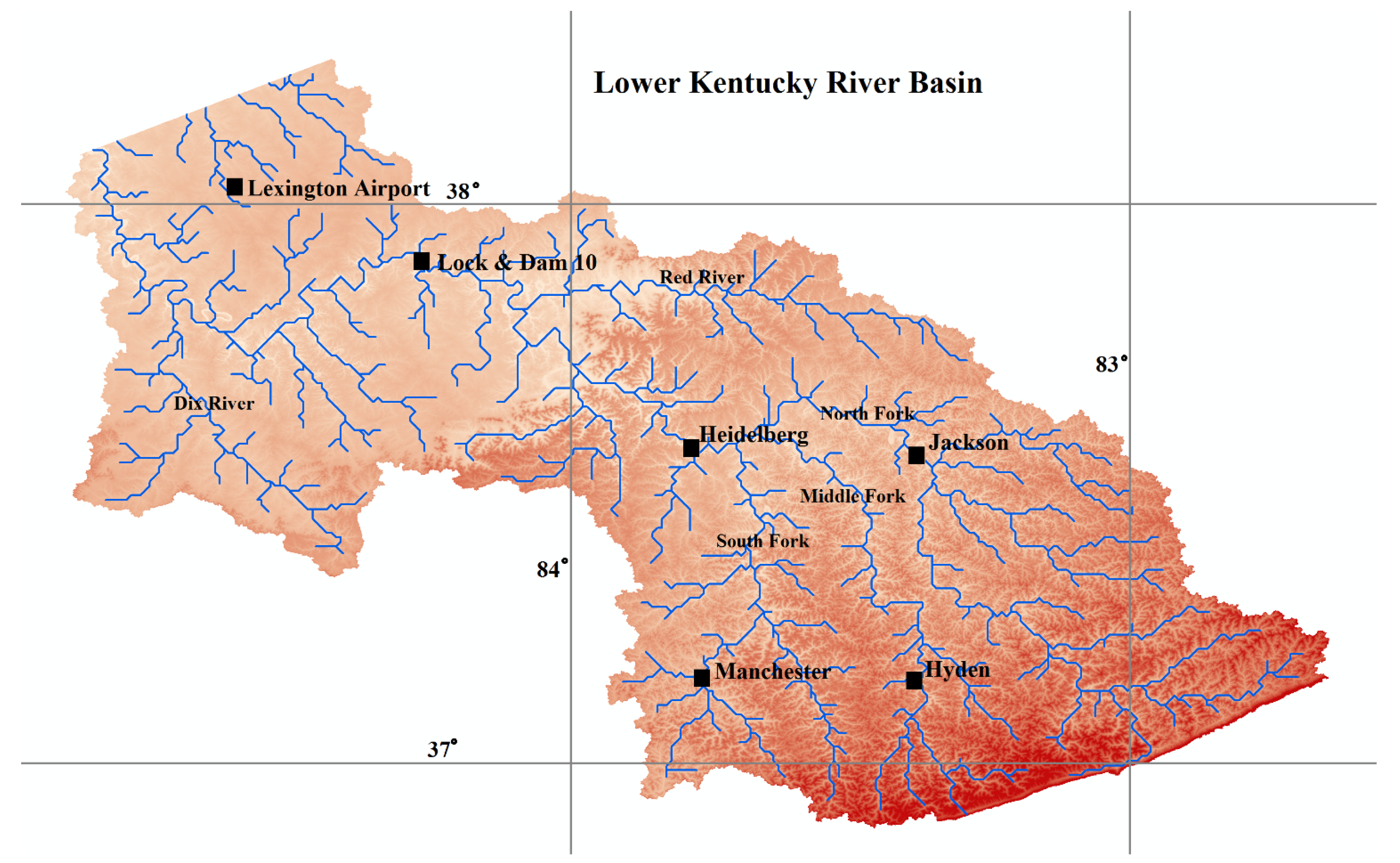
A diagram of the study area is shown in Figure 1. Data used for the study include daily average streamflow (m3/s) and average daily total rainfall (mm), with streamflow data being measured at a single location at Lock and Dam 10, south of Winchester, along the Kentucky River, and precipitation data being taken from an average of 5 gauges, at Manchester, Hyden, Jackson, Heidelberg, and Lexington Airport. The rain gauges at Manchester, Hyden, Jackson, and Heidelberg were chosen as their locations lie along the river network and directly supply to runoff at Lock and Dam 10. The rain gauge at Lexington Airport was chosen as it lies just north of Lock and Dam 10 and provides supplementary information regarding precipitation in the basin.
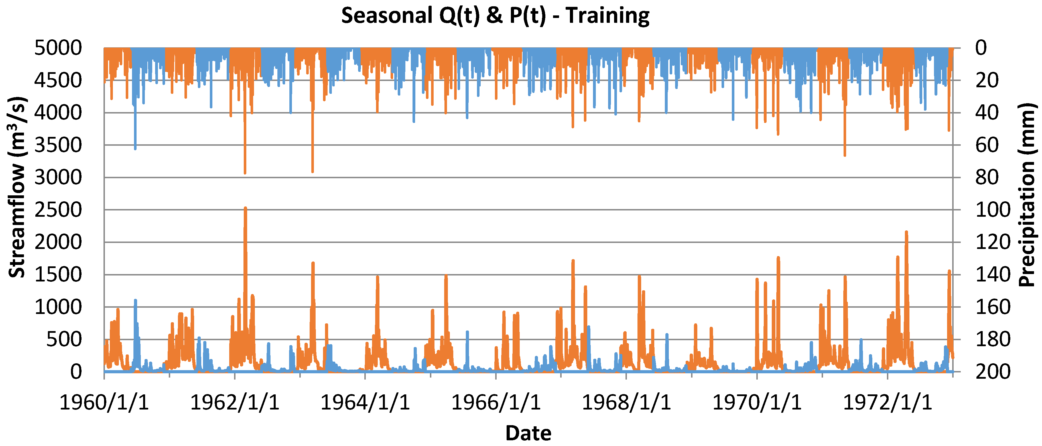
The Kentucky River Basin is a midsize catchment that covers 42 counties in Kentucky and encompasses a dense network of tributaries and streams with a length of 25,700 km. The major tributaries in the basin include: Eagle Creek, Dix River, Elkhorn Creek, Red River, North Fork Kentucky River, Middle Fork Kentucky River, and South Fork Kentucky River. The average slope of the Kentucky River is 0.13 m/km with the elevation of the river ranging from 243 to 305 m above sea level. The yearly average depth of rainfall for the basin is 1168 mm [24], with the climate being described as moist-continental. The average annual temperature within the basin is 13 °C with the minimum daily temperature being near −4 °C in January and February, and the maximum daily temperature being near 31 °C in July and August [25]. Along the Kentucky River there are a series of 14 locks constructed between the mid-nineteenth century to early twentieth century [26,27]. The drainage area influencing the outlet at Lock and Dam 10 is approximately 10,240.8 km2 [10] with the underlying geology being highly karst [28]. Streamflow and precipitation data were obtained from the USGS at waterdata.usgs.gov and consist of 9496 dates split into two 13 year periods from 1 January 1960 to 31 December 1972, and from 1 January 1977 to 31 December 1989. For each model, the first 13-year period was used for model training while the second 13-year period was used for model validation. Consistency in the datasets used allowed for more meaningful comparative assessment. The runoff and precipitation records for each of the two datasets are depicted in Figure 2 and Figure 3.

2.2. Linear Genetic Programming

LGP is a subset of genetic algorithms (GA), where evolutionary operators selectively breed and mutate a population of solutions to improve the best overall model. Algorithm 1 displays an image of a simple LGP with its corresponding algebraic structure. Unlike GA, which depicts equations in a representative tree-based structure, LGP portrays equations linearly, with the corresponding output from an initial instruction being further calculated through subsequent instructions, with instructions being represented as arithmetic operators. For example, in Algorithm 1 the LGP contains the arithmetic operators: plus (+), minus (−), square root (sqrt), and absolute value (abs). Within LGP, arithmetic operators are referred to as functional sets. For the study, the commercial software Discipulus™ [29] was utilized. Discipulus™ groups sets, on instructions, into 32-bit blocks of binary code allowing the software to interact directly with a machine’s registers and produce processing times that can be 60–200 faster than genetic algorithms. Individual solutions in LGP are referred to as programs as they are a sequence of instructions developed to perform a specified task.
Algorithm 1. Example of simple LGP (Linear Genetic Programming), with corresponding algebraic structure.
Water 08 00247 i001
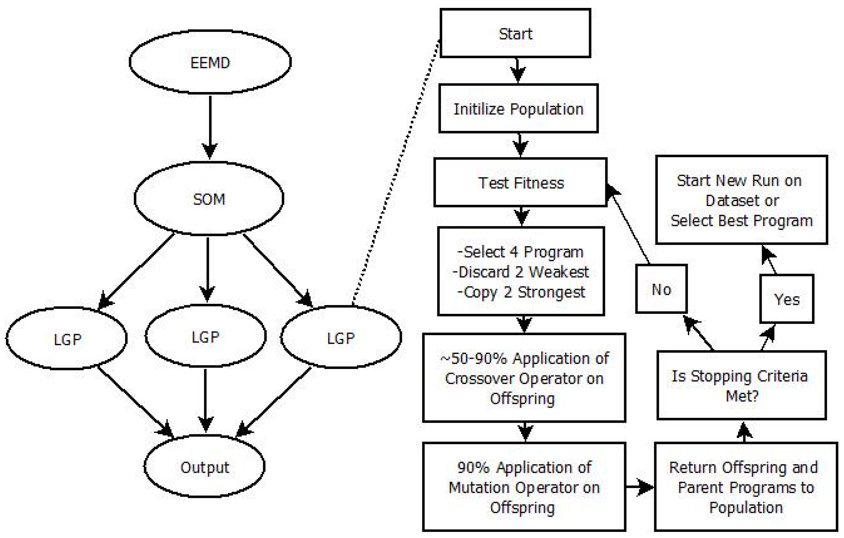
Creating models through LGP requires generating a random population of programs from the supplied input and output variables and improving those programs through a set of Darwinian operators that are applied over successive generations. The Darwinian operators come in the form of either mutation or crossover operators and are applied through a mating scheme referred to as tournament selection. Figure 4 depicts the mechanism of tournament selection along with the hybrid design implemented in this study. In tournament selection, four programs are randomly selected from the initial population and are evaluated based on their fitness. This study utilized the mean squared error (MSE) of individual programs as the statistical parameter for evaluating individual program fitness. Of the four programs selected, the two with the lowest MSE are selected and copied, creating two new offspring programs. The two programs that have a higher MSE, and thus are less fit, are discarded from the population entirely. The offspring programs then have the likelihood of exchanging algorithm information or generating new bits of algorithm through the application of either crossover or mutation operators. Crossover operators are the first to be applied and are done so with an application rate between 50% and 90% for individual project runs as selected randomly by the software. If a crossover operator is applied during a specific generation it will come in the form of either a homologous crossover operator, resulting in the exchange of instructions of equal length and starting location, or non-homologous, resulting in the exchange of instructions of different length and starting location. If a crossover operator was selected to be applied, homologous crossover operators were applied at a rate of 95% as to not bog down the processing time by creating a population of programs that vary extensively in length. The selection of the starting location is purely random, although it must be between individual instruction blocks which, as mentioned, are 32-bit blocks of binary code.
After the likelihood of crossover operators being applied, the application of mutation operators are applied with the purpose of generating new algorithmic information that may not have been present within the initial population. Unlike traditional applications of genetic algorithms, which aim to mimic a more natural evolution of the algorithmic population, the tournament selection scheme applied in this study applied mutation operators to roughly 90% of all offspring, allowing for an environment with a much higher rate of program evolution. Mutation operators come in three forms, with the selection of which one to be applied being chosen randomly and with equal likelihood. Of these, the block mutation operator discards an existing instruction block within an individual offspring program and regenerates the instruction block with new algorithmic information, the instruction mutation operator discards an individual instruction within an instruction block and generates a new algorithmic instruction to replace it, and the data mutation operator discards an individual terminal set (variable or constant) [11]. Once both a crossover and mutation operator have had the opportunity to be applied, both parents and both offspring programs are returned to the population for the possibility of being selected in further generations, allowing for the possibility of creating a new best-fit program. The stopping criteria for an individual program run was set at 1000 generations without best program improvement. The software allows for a multi-run environment so that multiple project runs could be implemented on the same input data, allowing for a wider selection of potential models for each objective.

2.3. Ensemble Empirical Mode Decomposition

The role of Empirical Mode Decomposition (EMD) is to decompose a natural, or synthetic, time-series into a number of separate oscillating trends, with each additional trend being the extracted zero-mean representation of the previous subcomponent. All subcomponents, except for the last extracted subcomponent, are referred to as Intrinsic Mode Functions (IMFs) with the final subcomponent portraying the overall trend of the data and being referred to as the residue. Together, each IMF, plus the final residual, sums to the original time-series. Individual components are labeled IMFs only if they meet two criteria. Firstly, for the component in question, the number of zero crossings and the number of extreme (minima and maxima) must be equal or differ by no more than one. Secondly, the mean value of the cubic spline interpolated envelope, defined as the space between the connected local maxima and connected local minima, must have a value near zero [30], with the degree of error allowed being set by the user. EMD is defined through the following set of rules:
(1)
Identify all local minima and local maxima of an original time-series x(t).
(2)
Create an upper envelope (eupper) by connecting all local maxima, and a lower envelope (elower) by connecting all local minima through the use of cubic spline interpolation.
(3)
Calculate the mean value of the upper and lower envelopes through the equation:
m ( t ) = [ e u p p e r ( t ) +   e l o w e r ( t ) 2 ]
(4)
Extract the computed mean value m(t) from the time-series x(t), with the difference being d(t):
d ( t ) = x ( t ) m ( t )
(5)
Check d(t) to see if it meets the defined requirements of an IMF. If the requirements are met then d(t) becomes the ith IMF denoted as ci(t) and the remaining x(t) is then referred to as the remaining residue r(t) denoted as r(t) = x(t) − ci(t) so that the process can continue and the next IMF can be extracted. If the requirements are not met then the process continues with d(t) replacing x(t) in the above equation and steps (1)–(5) being performed on the remaining d(t) until ci(t) is found.
(6)
Steps (1)–(5) are repeated until either r(t) becomes a monotonic function or the number of extrema becomes less than or equal to one.
(7)
Once completed, the original time-series x(t) can be expressed as the sum of the IMFs and the final residue r(t), with n representing the number of IMFs in the summation:
x ( t ) =   i = 1 n c i ( t ) + r ( t )
The iterative process of extracting IMFs through EMD portrays subcomponents representing different oscillating trends within the data that vary in amplitude are of successively lower frequency but maintain consistency in time. Each of these oscillating trends may reveal additional information related to the original time-series as they may be associated with different phenomena, known or unknown. For example, higher frequency trends are likely related to seasonal events, while lower frequency trends could be linked to yearly or decadal cycles. The total number of IMFs extracted per time-series is not user-specified and depends on the inherent nature of the original time-series. This study found, that for the two datasets utilized, EEMD was able to extract an equal number of IMFs. As EMD introduces the problem of mode mixing, an individual IMF having oscillations of highly varying amplitude or frequency, a modified version of EEMD presented by Torres et al. [31], was utilized for this study. The method relies on a set of user-defined variables, which are the noise standard deviation ( ε ), ensemble size (I), and the maximum number of iterations per realization. The method is applied on top of the existing structure of EMD, with the main focus being adding varying degrees of white noise to the original time-series and each extracted subcomponent while performing EMD on each until I is reached. Once I is reached, an ensemble average of the component in question is calculated and determined as the true IMF. Mathematically, this can be represented as:
(1)
Decompose through EMD I realizations of x(t) + ε · w 2 , where w represents white noise. Then take the ensemble average through:
c i ( t ) ¯ = 1 I 1 I c i ( t )
(2)
Then, instead of step (5), as above, calculate the remaining residue as:
r ( t )   =   x ( t )     c i ( t ) ¯

2.4. Self-Organizing Map

A Kohonen’s SOM is an unsupervised classification technique that requires no a priori knowledge of the data [32]. SOMs are a form of neural networks and consist of an input layer, an output layer, and connected weights between each input and output neuron. Neurons in the output layer are associated by topological relationships and are represented on a two-dimensional lattice. The goal of an SOM is to group input data by their common features through an unsupervised training algorithm, with the intention of mimicking the brain’s ability to store like information in closely associated neurons for greater efficiency through shorter synaptic connections.
An SOM is able to achieve data clustering through a number of steps that are repeated iteratively. The first step is the initialization of the connection weights with small random values. Next, competition takes place between output neurons for the lowest value squared Euclidean distance between the input and weight vectors. The winning neuron from competition, referred to as the best matching unit (BMU), marks the center of a topological neighborhood of excited neurons, where influence decreases the further the distance from the winning neuron. Lastly, excited neurons adjust their linked connected weights by minimizing the squared Euclidean distance between the input and weight vectors [17]. Mathematically, this is expressed as:
  • First finding the BMU:
    d j ( x ) =   i = 1 n ( x i w i ) 2
    where xi is the current input vector, wi is the current weight vector, and n is the number of weights.
  • Determining the radius of the neighborhood:
    σ ( t ) =   σ 0 e (   t λ )
    where t is the current iteration, λ is a time constant, and σ 0 is the radius of the map.
  • Determining the time constant:
    λ = s e t   n u m b e r   o f   i t e r a t i o n s r a d i u s   o f   t h e   m a p
  • Adjusting the weights of the neuron:
    w ( t + 1 ) = w ( t ) + Θ ( t ) L ( t ) ( x ( t ) w ( t ) )
    where w ( t + 1 ) is the new weight of a neuron.
  • Applying a learning rate to Equation (4) above:
    L ( t ) = L 0 e t λ
    where L0 is the learning rate from the previous step.
  • Recalculating the distance from the BMU
    Θ ( t ) = e d 2 2 σ 2 ( t )
    where d is the distance of an individual node from the BMU.
The squared Euclidean distance is used to avoid unnecessary computation time that may be imposed by the square root function. Equation (1)’s purpose is to provide a scale for comparing each node to the supplied input vector. Equations (2) and (5) employ exponential decay, where at t = 0 they are at their max and approach zero as t increases. Equation (4) is the learning function for the output nodes. The difference between the current input vector and current weight vector provides a means for nodes more dissimilar to the BMU to learn more than those that are similar. Equation (6) is designed to make nodes closer to the BMU learn more than nodes further away. For this study, the commercial software Viscovery SOMine [33] was implemented to perform SOM data clustering.

3. Model Development

Three separate objectives were demonstrated in this study. The first was to assess the effectiveness of LGP as a standalone application. LGP-1 though LGP-3 assessed LGP’s ability to predict daily streamflow with known precipitation. LGP-4 shows LGP’s ability to capture the observable low and high flow seasons present within the basin. LGP-5 depicts LGP’s ability to capture the rising and falling trends of the hydrograph. The second objective was to assess the functionality of implementing LGP into hybrid designs focusing on additional data processing. LGP-6 & LGP-7 implemented an SOM to classify the data into three clusters, with LGP models being run on each cluster and with the final output data from each model being combined. LGP-8 implemented EEMD to decompose the runoff time-series into a number of subcomponents to provide additional predictive information for LGP to capture daily streamflow amounts. LGP-9 preprocessed the data through both an SOM and EEMD to assess the effectiveness of clustering the decomposed runoff time-series and standard information for capturing streamflow through LGP. The third objective focuses on the practicality of the method as it assessed the effectiveness of using LGP and the hybrid design to predict streamflow multiple time-steps ahead. The best performing design is reported and is denoted as LGP 10 with the hybrid structure of EEMD-SOM-LGP.

3.1. LGP as a Standalone Application

The first objective of this study was to assess LGP as a standalone application for capturing streamflow. Furthermore, results were compared to published ANN models derived from the same dataset and with an identical objective. Numerous LGP models were derived. Appropriate input variable sets for the basin were determined from trial and error, based on the average impact and frequency of occurrence of individual variables in an initial model containing 10 days of previous runoff information and precipitation from the current day to nine days prior (Table S1 in Supplementary Material), along with the statistical performance of each produced model. Table 1 displays the most important of these produced models, along with including the best performing published ANN model that was trained through a genetic algorithm [10]. LGP-2 contains variables, all with a 100% frequency of occurrence. LGP-3 contains variables, all with an average impact above 1%.
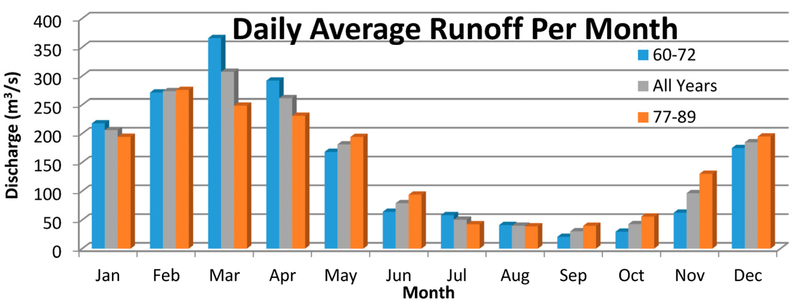
In addition, models were assessed based on their ability to capture the observable high and low flow periods (LGP-4), as well the rising and falling trends of the hydrograph (LGP-5). The input variables for these models are listed in Table 2. As seen in Figure 2 and Figure 3, clear variations in the catchment’s response to precipitation can be observed. This is further demonstrated by Figure 5, with the selection of the low flow season being from June through November and the high flow season being from December through May. LGP-4 utilized the input variable set from LGP-3 for direct comparison. In LGP-5, the rising and falling sections of the hydrograph were split at peak and base values, with each requiring at least 3 days of continuous trend. The falling section of LGP-5 incorporated an extra day of precipitation to account for the importance of incorporating delayed precipitation information on the falling sequences, as determined by trial and error (Tables S4 and S5).

3.2. LGP in Hybrid Application with EEMD and SOM

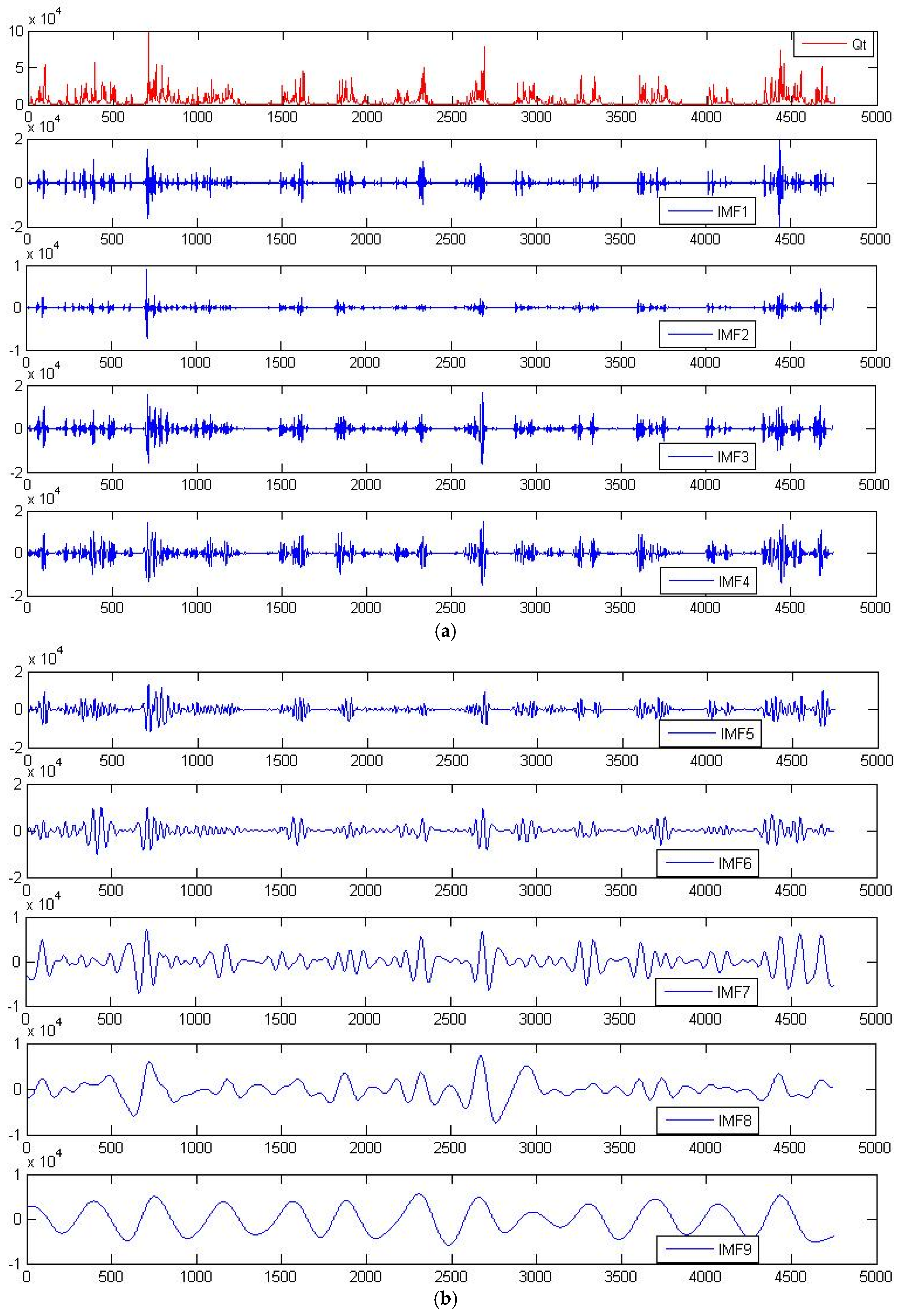
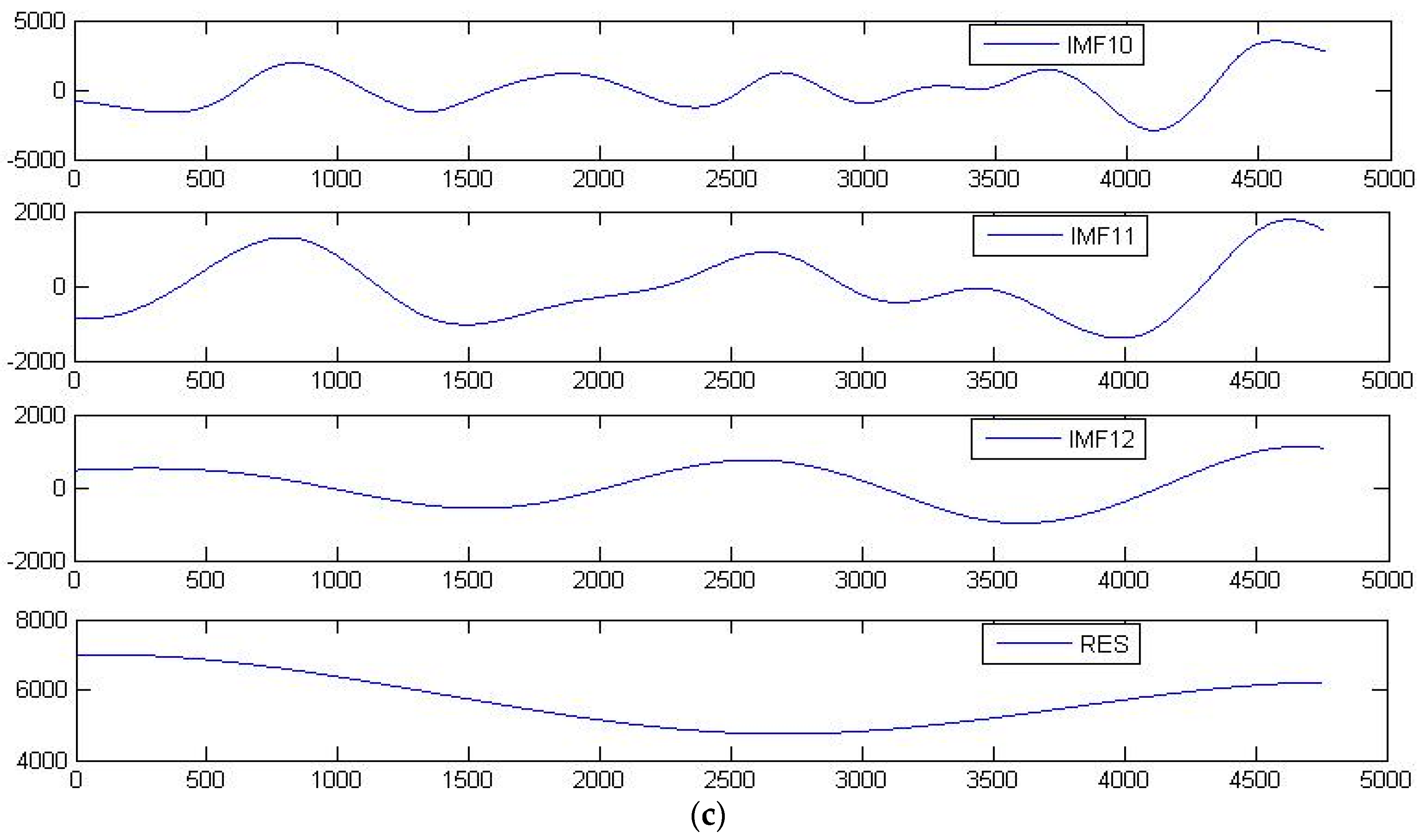
To improve the effectiveness of utilizing LGP for capturing streamflow, the second objective focused on implementing LGP models into hybrid designs. The data decomposition technique of EEMD was employed to deconstruct the original runoff time-series into a number of subcomponents, while an SOM was utilized to classify the input space into a number of classes, with separate LGP models being run on each. Figure 6 depicts the 12 IMFs derived from EEMD for the validation dataset. As can be observed, the high-frequency IMFs display periods of increased volatility before and after heavy flows. EEMD was implemented to improve the autocorrelation of runoff information and to give LGP more information when associating past flows with capturing output information. Although the number of generated IMFs cannot be user-specified, an equal number of IMFs were created for both the training and validation datasets. The SOM design consisted of mapping the input vectors onto a two-dimensional 1000 neuron lattice, with each SOM model consisting of 3 or 4 classes. The classes reflected a class of low precipitation and low flows, a class of high precipitation and medium flows, a class of low precipitation and increasing high volume flows, and a class of low precipitation and decreasing high volume flows (with the latter two classes being combined in the 3 class models).
LGP-6 & LGP-7 were created for direct comparison with LGP-2 & LGP-3 and utilized an SOM before LGP application. Each model was split into 3 classes with the output data being combined for analysis. LGP-8 utilized EEMD-derived runoff information to assess its impact on the performance of LGP for capturing streamflow within the basin. IMF components were stretched to the previous 3 days (i.e., IMF 1(t−1), IMF 1(t−2), IMF 1(t−3), IMF 2(t−1) … etc.). Like LGP-2 & LGP-3, which were the best-performing models from a set of models with different variable sets, the variable set for LGP-8 was determined through trial and error based on the average impact and frequency of occurrence in an initial model (Table S8) and numerous subsequently created models (Tables S9 and S10). It was found that utilizing the first 5 IMFs contributed to the greatest statistical performance when utilizing LGP to capture streamflow, which was further implied by a significant tapering off in the average impact and frequency of occurrence for IMFs 6 through 12. It is noted that the selection of IMFs is largely based on the researcher’s a priori knowledge of the original time-series [34]. LGP-9 implemented the variable set from LGP-8, but with the addition of utilizing an SOM to cluster the standard and EEMD-derived input data into 4 separate classes, with the output data being combined for analysis. Table 3 depicts the input variables for each model.

3.3. Practicality of the Method for Forecasting Multiple Time-Steps Ahead

The third objective focused on the practicality of the method with the goal to assess the effectiveness of the EEMD-SOM-LGP hybrid design to predict streamflow multiple days ahead. Other designs, such as LGP as a standalone and EEMD-LGP, were explored, but only the best performing is being reported. Predictions were made for up to four days ahead, with output data from the previous model being used as input data in predicting the next step. The EEMD IMF component, as deemed most influential from LGP-8, were incorporated within the models and were clustered into three classes through an SOM, with individual LGP applications being run on each class. Table 4 depicts the input variables for LGP-10 and LGP-11.

3.4. Model Performance

A set of standard statistical measures were employed to evaluate the performance of each model developed, with each model simply being the best fit program from each project. The applied measures include the average absolute relative error (AARE), Pearson’s correlation coefficient (R), Nash-Sutcliff efficiency (E), normalized mean bias error (NMBE), normalized root mean square error (NRMSE), mean error in estimating peak flow (%MF), and the persistence coefficient (Eper). These measures are portrayed through the following equations:
AARE ( % ) =   1 N t = 1 N | Q o b s ( t ) Q ( t ) Q o b s ( t ) | x   100
R =   t = 1 N ( Q o b s ( t ) Q o b s . m e a n ) ( Q o b s ( t ) Q m e a n ) t = 1 N ( Q o b s ( t ) Q o b s . m e a n ) 2 ( Q ( t ) Q m e a n ) 2
E =   ( t = 1 N ( Q o b s ( t ) Q o b s . m e a n ) 2 ) ( t = 1 N ( Q ( t ) Q o b s ( t ) ) 2 ) ( t = 1 N ( Q o b s ( t ) Q o b s . m e a n ) 2 )
NMBE   ( % ) =   1 N t = 1 N ( Q ( t ) Q o b s ( t ) ) 1 N t = 1 N ( Q o b s ( t ) )   x   100
NRMSE =   [ 1 N t = 1 N ( Q ( t ) Q o b s ( t ) ) 2 ] 1 / 2 1 N t = 1 N ( Q o b s ( t ) )
%MF =   Q m a x Q o b s . m a x Q o b s . m a x   x   100
E per =   ( t = 1 N ( Q o b s ( t ) Q o b s ( t 1 ) ) 2 )   ( d = 1 N ( Q ( t ) Q o b s ( t ) ) 2 ) ( t = 1 N ( Q o b s ( t ) Q o b s ( t 1 ) ) 2 )
Statistical parameters include the predicted flow Q(t) for each day t, the observed flow Qobs(t) for each day t, the number of days included in the dataset N, the mean estimated flow Qmean, the mean observed flow Qobs.mean, the maximum estimated flow Qmax, and the maximum observed flow Qobs.max. The parameter Qobs(t−1) refers to the observed runoff measurement from the previous day.
Each statistical measure provides unique insight into the performance of the models. The AARE provides an unbiased measure for determining a model’s predictive capability through averaging the absolute value of each day’s relative error. The correlation coefficient describes the strength of the linear relationship between predicted and observed flow. The Nash and Sutcliffe coefficient of efficiency (E) provides insight into the linear relationship between predicted and observed flow but also allows describing variance within a model by giving us an indication of the percent of data that falls along the line of best fit [35]. Moriasi et al. [36] note that E values above 0.75 are very satisfactory for streamflow prediction. The NMBE describes a model’s predictive bias. The NRMSE measures the difference between predicted and observed values by normalizing the sample standard deviation, giving an idea of the model’s ability to predict values away from the mean. Error amongst peak predicted and observed flow (%MF) gives engineers a general idea of a model’s reliability for estimations pertaining to hydrologic design. Finally, Eper was calculated, which gives the relative error between the difference in the observed flow and the observed flow of the day before and the difference of the predicted and observed flow.

4. Results and Discussion

Results for the ability of each model to capture discharge at Lock and Dam 10 along the Kentucky River are listed below for the different objectives of this study. Each model was evaluated based on the seven statistical parameters discussed in the previous section.
Table 5 and Table 6 present the performance parameters for the first objective of models, which focused on assessing LGP’s ability to capture streamflow within the basin. LGP-1 shows the strong autocorrelation of runoff information when capturing streamflow within the models. Conversely, it was found that oversupplying LGP models with too many days of precipitation information lead to significant reductions in the performance of the models. For example, including P(t), P(t−1), and P(t−2) with three days of past runoff resulted in an AARE of 50.23 and NMBE of 2.90. This model is labeled LGP 1.7 and can be found in the supplementary material in Tables S2 and S3. It is noted in [37] that including precipitation beyond the catchments lag time can lead to a loss in the predictive capability of data-driven models. The lag time to Lock and Dam 10 has been reported as two days [38]. LGP-2 & LGP-3 display the strength of LGP for creating data-driven models capturing streamflow. Although LGP-2 displayed a stronger AARE and with fewer variables, LGP-3 outperformed LGP-2 in most of the other statistical parameters, aside from capturing the peak flow in the dataset. When compared to the best performing ANN model published in [10], LGP-2 & LGP-3 posted stronger validation AARE values, with similar statistical values for the other validation set parameters. The strongest ANN model published in [10] can be found in Table 5. It was trained through a genetic algorithm and run over the same datasets as the models produced in this study.
Modeling the low and high flow seasons for the basin separately shows a strong under-prediction during the low flow seasons, as indicated by the NMBE in LGP-4. Of the dates associated with the highest relative error in LGP-2 & LGP-3, a majority occurred during months of low flow, suggesting an altered dynamic to the environment during these periods, with potential causes being increased infiltration from the underlying karst geology as the ground becomes less saturated from loss of snowmelt and warmth, increased evaporation of water from pooling along the lock system, and increased municipal and irrigational usage during summer months. LGP-5 shows a greater ease for LGP to model the falling portions of the hydrograph in comparison with the rising trends. Examining the rising portions of the hydrograph’s output shows large degrees of relative error associated with the over-prediction of streamflow on days of small changes in actual streamflow after heavy precipitation, with these events occurring during the low flow season. Additionally, modeling the effect of precipitation error on model performance shows a greater degree of error associated with the undervalued precipitation estimations as compared to overestimations (Tables S6 and S7).
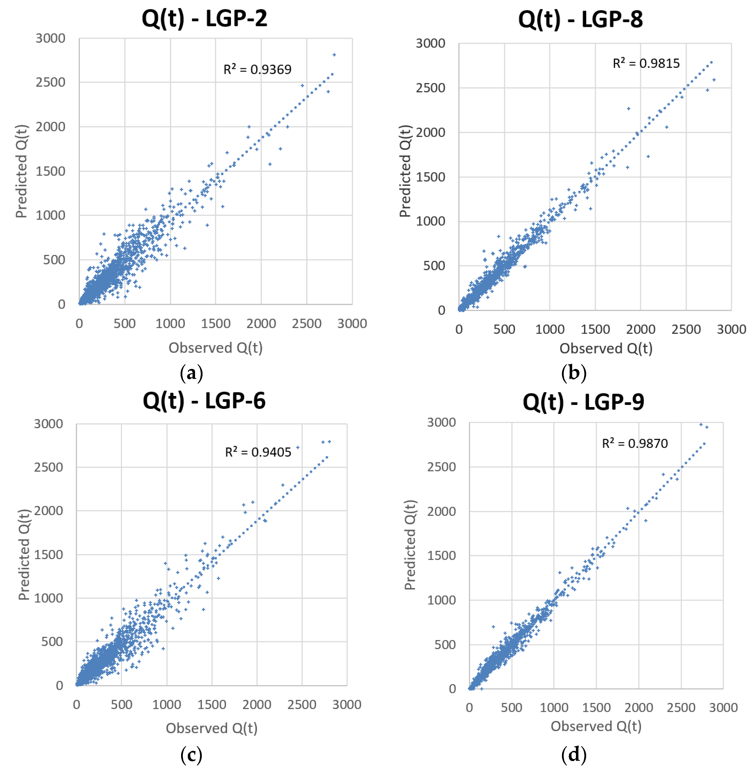
LGP-6 through LGP-9 were assessed incorporating LGP into hybrid designs, with the results presented in Table 7. LGP-6 & LGP-7 were created for direct comparison with LGP-2 & LGP-3 and included an SOM to classify the input space before LGP application on each class. When comparing LGP-6 with LGP-2 it is seen that classifying the input space did not provide a significant reward for the added computation requirement, as some parameters slightly improved (NRMSE, Eper, E) and others regressed (AARE, NMBE). Comparing LGP-7 to LGP-3 resulted in more parameters that improved, but again, the improvements were not enough to justify the added computation requirement and time. LGP-8, which utilized IMF data derived from EEMD in addition to standard rainfall and precipitation information, showed major improvement in reducing AARE and improving E & Eper, while better-predicting values further from the mean, as indicated by its NRMSE. From the set of EEMD included models that resulted in LGP-8, consistently stronger AARE, E, I, NRMSE, and Eper values were found, although it appeared to create a negative bias for %MF. These models, including others, are included in the supplementary material. Further improvement was seen when an SOM was utilized to classify EEMD and standard information before LGP application, as indicated by LGP-9. Of the different designs presented, LGP-9 resulted in the largest reduction in error, with an AARE of 10.122, the strongest Nash-Sutcliffe of 0.987, strongest Eper of 0.931, the strongest ability to predict values away from the mean, with an NRMSE of 0.182, and very low magnitude of over-predicting, with and NMBE of 0.161. Utilizing an SOM in conjunction with EEMD-derived runoff information was shown to significantly improve the performance of models created through LGP. Figure 7 shows a scatter-plot comparison between LGP-2, LGP-6, LGP-8, and LGP-9 for capturing streamflow.
Table 8 displays a comparison of the low, medium, and high magnitude flows for select models. Intervals were derived from generated intervals of streamflow information through an SOM, but were also guided through observable values. The flow intervals composed of low flows between 0 and 28.2 m3/s, medium flows between 28.2 and 282.3 m3/s, and high flows above 282.3 m3/s. LGP-2, which utilized LGP as a standalone application, resulted in an extremely strong AARE, which was not reproduced for any other LGP standalone models created during trial and error, which likely signifies that it is an extreme outlier linear genetic program for this individual basin. LGP-3, LGP-8, & LGP-9 each show more difficulty in predicting low magnitude flows compared to medium and high magnitude flows, with LGP-9 reporting the best results for each interval.
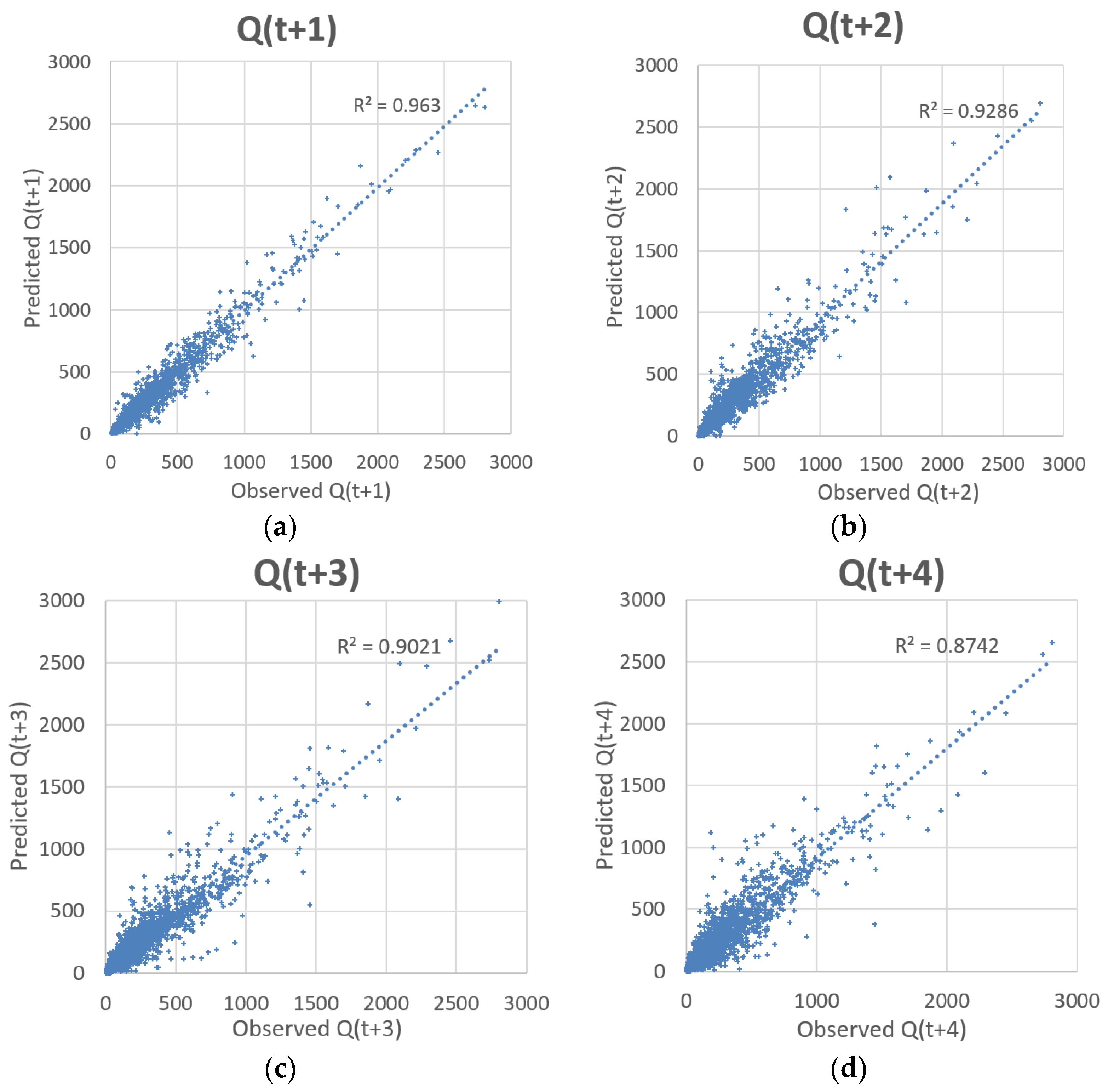
The third and primary objective of this study was to determine the practicality of the method by assessing its ability to predict multiple time-steps ahead. Table 9 displays the statistical performance of the EEMD-SOM-LGP architecture for predicting streamflow at Lock and Dam 10 along the Kentucky River Basin up to 4 days ahead. The hybrid design depicts strong values for predicting streamflow up to two days ahead with acceptable values that can give a good indication on streamflow for days three and four. Figure 8 compares the ability of the EEMD-SOM-LGP design to predict streamflow at different time-steps.
Other model designs were assessed but are not reported (Tables S11–S18). For example, using LGP as a standalone was deemed non-effective, as considerable lag developed between observed and predicted values. To account for the need to include the basin’s response to precipitation when using LGP as a standalone application, models could incorporate forecasted precipitation information, although at the expense of new issues. Utilizing an EEMD-LGP design eliminated this lag and returned strong results, although not as effective as when incorporating an SOM into the model design. For example, at Q(t+3), the EEMD-LGP model returned an AARE of 47.832, an E of 0.889, and an Eper of 0.522, while the EEMD-SOM-LGP design returned an AARE of 43.365, an E of 0.902, and an Eper of 0.591 at Q(t+3). Utilizing the EEMD-SOM-LGP design also minimized the negative effect on %MF, as values without the application of the SOM were all negative and in double digits. For comparative purposes, these models can be found in the supplementary material. Figure 9 compares LGP-10 with LGP as a standalone application for predicting streamflow at three days ahead.

5. Conclusions

This study focused on assessing the effectiveness of LGP as a standalone application and in hybrid designs with EEDM and an SOM to capture streamflow, while also focusing on the ability of the hybrid design to forecast streamflow multiple time-steps ahead. Daily average rainfall and streamflow data from the Kentucky River Basin were utilized to develop each of the models, with a number of different statistical parameters being used to evaluate their performance.
The findings from this study suggest that LGP works very well when utilized with EEMD-derived runoff data, and even better when an SOM is utilized to create separate data classes composed of EEMD-derived runoff information and observed values with each class being run as a separate model. Selecting the appropriate IMFs is largely up to the user’s knowledge of the data, with the five highest frequency IMFs being determined to provide the greatest degree of predictive performance in regards to this catchment.
Utilizing LGP as a standalone application to capture streamflow resulted in very similar findings when compared to the best performing ANN model from [10], which was developed over the same dataset and input variables and trained through a genetic algorithm. Classifying the input space through an SOM before modeling each class through LGP did not prove to be worthwhile without the inclusion of EEMD-derived runoff subcomponents. When EEMD-derived runoff subcomponents were utilized with LGP, all the statistical parameters significantly improved, aside from %MF. Including all three techniques together in an EEMD-SOM-LGP structure resulted in the strongest performance of all the reported models. The design also proved highly effective for making predictions multiple time-steps ahead.
The fast processing environments of LGP, SOM, and EEMD make them very good data-driven techniques for forecast modeling, especially when utilized together. Streamlining all the techniques into a single application would benefit forecast modelers. As the findings from this study are preliminary in nature, they should be reinforced on additional basins and for forecasting other natural signals. Also, developing a more comprehensive method for the selection of the appropriate IMF components could be investigated and implemented, likely further improving results.

Supplementary Materials

The following are available online at www.mdpi.com/2073-4441/8/6/247/s1. Table S1: Average impact and frequency of occurrence for of input parameters of models that used LGP as a standalone application; Table S2: Variables included in LGP standalone models; Table S3: Statistical parameters for LGP standalone models in Table 2; Table S4: Input variables for models depicted separated Rising/Falling trends using LGP as a standalone application; Table S5: Statistical parameters for models depicted separated Rising/Falling trends using LGP as a standalone application as depicted in Table S4; Table S6: Input Variables for tested error in precipitation record using LGP as a standalone application; Table S7: Statistical parameters for tested error in precipitation record using LGP as a standalone application as depicted in Table S6; Table S8: Frequency and average impact of input variables from models using EEMD-LGP design to capture streamflow; Table S9: Input variables for all tested EEMD-LGP models; Table S10: Statistical parameters for EEMD-LGP models depicted in Table S9; Table S11: Output and input variables for LGP as standalone application for predicting ahead; Table S12: Statistical parameters for LGP standalone models for predicting ahead as depicted in Table S11; Table S13: Output and input variables for LGP as standalone with updated precipitation record to account for delays between actual and predicted streamflow (forecasted rainfall would need to be used); Table S14: Statistical parameters for models described in Table S13 which used LGP as a standalone application to predict streamflow multiple time-steps ahead; Table S15: Output and input variables EEMD-LGP models predicting ahead; Table S16: Statistical parameters for models described in Table S15 which used a EEMD-LGP design and the known precipitation record to predict streamflow multiple time-steps ahead; Table S17: Output and input variables for EEMD-LGP models that would require forecasted precipitation; Table S18: Statistical parameters for models in Table S17 which used a EEMD-LGP design to predict streamflow multiple time steaps ahead while requiring forecasted precipitation data.

Author Contributions

Jonathan T. Barge: Research and literature review, model implementation, ideas for adoption of hybrid designs (EEMD, SOM) to improve model performance, primary author of manuscript. Hatim O. Sharif: Original idea for use of LGP in streamflow forecasting at location to compare with published ANN models, data acquisition, consultation on how application can be used in different ways and how to improve manuscript, assisted in literature review, secondary author of manuscript.

Conflicts of Interest

The authors declare no conflict of interest.

References

  1. Vojtěch, K.; Hanel, M.; Máca, P.; Kuráž, M.; Pech, P. Incorporating basic hydrological concepts into genetic programming for rainfall-runoff forecasting. Computing 2013, 95, 363–380. [Google Scholar]
  2. Mulvaney, T.J. On the use of self-registering rain and flood gauges in making observations of the relations of rainfall and flood discharges in a given catchment. Proc. Inst. Civ. Eng. Irel. 1851, 4, 18–33. [Google Scholar]
  3. Beven, K.J. Rainfall-Runoff Modelling: The Primer; John Wiley & Sons: Lancaster, UK, 2011. [Google Scholar]
  4. Nourani, V.; Özgür, K.; Mehdi, K. Two hybrid artificial intelligence approaches for modeling rainfall-runoff process. J. Hydrol. 2011, 402, 41–59. [Google Scholar] [CrossRef]
  5. Babovic, V.; Keijzer, M. Rainfall runoff modelling based on genetic programming. Hydrol. Res. 2002, 5, 331–346. [Google Scholar]
  6. Makkeasorn, A.; Chang, N.-B.; Zhou, X. Short-term streamflow forecasting with global climate change implications—A comparative study between genetic programming and neural network models. J. Hydrol. 2008, 352, 336–354. [Google Scholar] [CrossRef]
  7. Parasuraman, K.; Amin, E.; Sean, K.C. Modelling the dynamics of the evapotranspiration process using genetic programming. Hydrol. Sci. J. 2007, 52, 563–578. [Google Scholar] [CrossRef]
  8. Aytek, A.; Murat, A. An application of artificial intelligence for rainfall-runoff modeling. J. Earth Syst. Sci. 2008, 117, 145–155. [Google Scholar] [CrossRef]
  9. Mehr, A.D.; Ercan, K.; Ehsan, O. Streamflow prediction using linear genetic programming in comparison with a neuro-wavelet technique. J. Hydrol. 2013, 505, 240–249. [Google Scholar] [CrossRef]
  10. Srinivasulu, S.; Ashu, J. A comparative analysis of training methods for artificial neural network rainfall-runoff models. Appl. Soft Comput. 2006, 6, 295–306. [Google Scholar] [CrossRef]
  11. Poli, R.; McPhee, N.; Langdon, W. A Field Guide to Genetic Programming; Creative Commons: San Francisco, CA, USA, 2008. [Google Scholar]
  12. Chang, L.C.; Shen, H.Y.; Wang, Y.F.; Huang, J.Y.; Lin, Y.T. Clustering-based hybrid inundation model for forecasting flood inundation depths. J. Hydrol. 2010, 385, 257–268. [Google Scholar] [CrossRef]
  13. Nourani, V.; Mehdi, K.; Mohammad, T.A. Hybrid wavelet-genetic programming approach to optimize ANN modeling of rainfall-runoff Process. J. Hydrol. Eng. 2011, 17, 724–741. [Google Scholar] [CrossRef]
  14. Kisi, O.; Jalal, S. Precipitation forecasting using wavelet-genetic programming and wavelet-neuro-fuzzy conjunction models. Water Resour. Manag. 2011, 25, 3135–3152. [Google Scholar] [CrossRef]
  15. Wang, W.; Xu, D.M.; Chau, K.W.; Chen, S. Improved annual rainfall-runoff forecasting using PSO–SVM model based on EEMD. J. Hydroinform. 2013, 15, 1377–1390. [Google Scholar] [CrossRef]
  16. Di, C.; Yang, X.; Wang, X. A Four-Stage Hybrid Model for Hydrological Time Series Forecasting. PLoS ONE 2014, 9, e104663. [Google Scholar] [CrossRef] [PubMed]
  17. Murtagh, F.; Hernández-Pajares, M. The Kohonen self-organizing map method: An assessment. J. Classif. 1995, 12, 165–190. [Google Scholar] [CrossRef]
  18. Ismail, S.; Ani, S.; Ruhaidah, S. A hybrid model of self-organizing maps (SOM) and least square support vector machine (LSSVM) for time-series forecasting. Expert Syst. Appl. 2011, 38, 10574–10578. [Google Scholar] [CrossRef]
  19. Ju, Q.; Yu, Z.; Hao, Z.; Ou, G.; Zhao, J.; Liu, D. Division-based rainfall-runoff simulations with BP neural networks and Xinanjiang model. Neurocomputing 2009, 72, 2873–2883. [Google Scholar] [CrossRef]
  20. Jain, A.; Sanaga, S. Integrated approach to model decomposed flow hydrograph using artificial neural network and conceptual techniques. J. Hydrol. 2006, 317, 291–306. [Google Scholar] [CrossRef]
  21. Weissling, B.P.; Xie, H. MODIS Biophysical States and NEXRAD Precipitation in a Statistical Evaluation of Antecedent Moisture Condition and Streamflow. J. Am. Water Resour. Assoc. 2009, 45, 419–433. [Google Scholar] [CrossRef]
  22. Chen, P.-A.; Chang, L.-C.; Chang, F.-J. Reinforced recurrent neural networks for multi-step-ahead flood forecasts. J. Hydrol. 2013, 497, 71–79. [Google Scholar] [CrossRef]
  23. Yang, J.-S.; Yu, S.-P.; Liu, G.-M. Multi-step-ahead predictor design for effective long-term forecast of hydrological signals using a novel wavelet neural network hybrid model. Hydrol. Earth Syst. Sci. 2013, 17, 4981–4993. [Google Scholar] [CrossRef]
  24. Kentucky Geological Survey, Kentucky River Basin Map and Chart by Daniel I. Carey. 2015. Available online: http://kgs.uky.edu/kgsweb/olops/pub/kgs/mc188_12.pdf (accessed on 20 May 2015).
  25. USGS (U.S. Geologic Survey). Water-quality assessment of the Kentucky River Basin, Kentucky—Analysis of available surface-water-quality data through 1986. In National Water-Quality Assessment; USGS Water-Supply Paper 2351; USGS: Reston, VA, USA, 1995. [Google Scholar]
  26. Kentucky River Authority. Kentucky River History—Locks and Dams. 2015. Available online: http://finance.ky.gov/offices/Pages/LocksandDams.aspx (accessed on 20 May 2015). [Google Scholar]
  27. Johnson, L.R.; Charles, E.P. Kentucky River Development: The Commonwealth’s Waterway; Louisville District, U.S. Army Corps of Engineers: Louisville, KY, USA, 1999.
  28. Currens, J.C. Model Ordinance for Development on Karst in Kentucky. In Kentucky Geological Survey; University of Kentucky: Lexington, KY, USA, 2009. [Google Scholar]
  29. Deschaine, L.M.; Frank, D.F. Comparison of Discipulus™ Linear Genetic Programming Soft-ware with Support Vector Machines, Classification Trees, Neural Networks and Human Experts. In White Paper; RML Technologies, Inc.: Boulder, CO, USA, 2004. [Google Scholar]
  30. Wu, Z.H.; Huang, N.E.; Chen, X. The multi-dimensional ensemble empirical mode decomposition method. Adv. Adapt. Data Anal. 2009, 1, 339–372. [Google Scholar] [CrossRef]
  31. Torres, M.E.; Colominas, M.A.; Schlotthauer, G.; Flandrin, P. A complete ensemble empirical mode decomposition with adaptive noise. In Proceedings of the IEEE International Conference on Acoustics, Speech and Signal Processing (ICASSP), Prague, Czech Republic, 22–27 May 2011.
  32. Kohonen, T. The self-organizing map. Proc. IEEE 1990, 78, 1464–1480. [Google Scholar] [CrossRef]
  33. Kastberger, G.; Gerhard, K. Visualization of multiple influences on ocellar flight control in giant honeybees with the data-mining tool Viscovery SOMine. Behav. Res. Methods Instrum. Comput. 2000, 32, 157–168. [Google Scholar] [CrossRef] [PubMed]
  34. Gallego, J.A.; Rocon, E.; Koutsou, A.D.; Pons, J.L. Analysis of kinematic data in pathological tremor with the Hilbert-Huang transform. In Proceedings of the 5th International IEEE/EMBS Conference on Neural Engineering (NER), Cancun, Mexico, 27 April–1 May 2011.
  35. Nash, J.E.; Sutcliffe, J.V. River flow forecasting through conceptual models part I—A discussion of principles. J. Hydrol. 1970, 10, 282–290. [Google Scholar] [CrossRef]
  36. Moriasi, D.N.; Arnold, J.G.; Van Leiw, M.W.; Binger, R.L.; Harmel, R.D.; Veith, T.L. Model evaluation guidelines for systematic quantification of accuracy in watershed simulations. Trans. ASABE 2007, 50, 885–900. [Google Scholar] [CrossRef]
  37. De Vos, N.J.; Rientjes, T.H.M. Constraints of artificial neural networks for rainfall-runoff modelling: Trade-offs in hydrological state representation and model evaluation. Hydrol. Earth Syst. Sci. Discuss. 2005, 2, 365–415. [Google Scholar] [CrossRef]
  38. Ashu, J.; Sudheer, K.P.; Sanaga, S. Identification of physical processes inherent in artificial neural network rainfall runoff models. Hydrol. Process. 2004, 18, 571–581. [Google Scholar]
Figure 1. Map of Lower Kentucky River Basin.
Water 08 00247 g001
Figure 2. Streamflow and precipitation record for the training dataset. Red represents the high flow seasons while blue represents the low flow seasons.
Water 08 00247 g002
Figure 3. Streamflow and precipitation record for the validation dataset. Red represents the high flow seasons while blue represents the low flow seasons.
Water 08 00247 g003
Figure 4. Ensemble Empirical Mode Decomposition-Self-Organizing Map-Linear Genetic Programming structure with tournament selection in LGP.
Water 08 00247 g004
Figure 5. Each month’s average daily average discharge.
Water 08 00247 g005
Figure 6. Runoff time-series and IMF (Intrinsic Mode Functions) signal components for validation dataset. (a) Original validation runoff time-series and first 4 IMF components; (b) IMF components 5 through 9; (c) IMF components 10 through 12 and the final residue.
Water 08 00247 g006aWater 08 00247 g006b
Figure 7. Scatter plots of observed vs. predicted for select models. An improved fit can be seen in the EEMD-LGP (LGP-8) and EEMD-SOM-LGP (LGP-9) models for capturing streamflow. (a) LGP as standalone application; (b) SOM-LGP; (c) EEMD-LGP; (d) EEMD-SOM-LGP.
Water 08 00247 g007
Figure 8. Q(t+3) predicted vs observed for LGP-10 and LGP as a standalone.
Water 08 00247 g008
Figure 9. Scatter plots of observed vs. predicted for models in LGP-10. (a) Streamflow at 1 day ahead; (b) streamflow at 2 days ahead; (c) streamflow at 3 days ahead; (d) streamflow at 4 days ahead.
Water 08 00247 g009
Table 1. Input variables included for LGP as a standalone application along with comparative ANN model.
ModelInput Variables
LGP-1Q(t−1), Q(t−2), Q(t−3)
LGP-2P(t), Q(t−1), Q(t−2)
LGP-3P(t), P(t−1), Q(t−1), Q(t−2), Q(t−3)
ANN [10]P(t), P(t−1), P(t−2), Q(t−1), Q(t−2)
Table 2. Input variables for LGP as standalone application in capturing different aspects of hydrograph.
ModelInput Variables
LGP-4High SeasonP(t), P(t−1), Q(t−1), Q(t−2), Q(t−3)
Low SeasonP(t), P(t−1), Q(t−1), Q(t−2), Q(t−3)
LGP-5Rising TrendsP(t), Q(t−1), Q(t−2)
Falling TrendsP(t), P(t−1), Q(t−1), Q(t−2)
Table 3. Input variables LGP models in hybrid designs untilizing EEMD and SOM.
ModelHybridInput Variables
LGP-6SOM-LGPP(t), Q(t−1), Q(t−2)
LGP-7SOM-LGPP(t), P(t−1), Q(t−1), Q(t−2), Q(t−3)
LGP-8EEMD-LGPP(t), Q(t−1), Q(t−2), Q(t−3) *imf set
LGP-9EEMD-SOM-LGPP(t), Q(t−1), Q(t−2), Q(t−3) *imf set
Notes: *imf set: IMF 1(t−1), IMF 1(t−2), IMF 1(t−3), IMF 2(t−1), IMF 2(t−2), IMF 2(t−3), IMF 3(t−1), IMF 3(t−2), IMF 3(t−3), IMF 4(t−1), IMF 4(t−2), IMF 4(t−3), IMF 5(t−1), IMF 5(t−2), IMF 5(t−3).
Table 4. Output and Input variables for EEMD-SOM-LGP models designed to predict ahead (LGP-10).
Output Input Variables for LGP-10
Q(t+1)P(t), Qpred(t), Q(t−1), Q(t−2), Q(t−3), *imfs
Q(t+2)P(t), Qpred(t+1), Qpred(t), Q(t−1), Q(t−2), Q(t−3), *imfs
Q(t+3)P(t), Qpred(t+2), Qpred(t+1), Qpred(t), Q(t−1), Q(t−2), Q(t−3), *imfs
Q(t+4)P(t), Qpred(t+3), Qpred(t+2), Qpred(t+1), Qpred(t), Q(t−1), Q(t−2), Q(t−3), *imfs
Notes: *imfs: IMF 1(t−1), IMF 1(t−2), IMF 1(t−3), IMF 2(t−1), IMF 2(t−2), IMF 2(t−3), IMF 3(t−1), IMF 3(t−2), IMF 3(t−3), IMF 4(t−1), IMF 4(t−2), IMF 4(t−3), IMF 5(t−1), IMF 5(t−2), IMF 5(t−3).
Table 5. Statistical measures for LGP standalone application.
Model Set 1AAREERNMBENRMSE%MFEper
LGP-1Training38.2610.9110.955−0.0220.485−3.9340.477
Validation38.3050.9010.9490.0830.502−3.5300.477
LGP-2Training17.2230.9430.971−0.8280.387−12.7400.666
Validation17.1180.9370.968−0.9050.4010.1560.666
LGP-3Training22.0260.9420.9700.6150.393−14.6630.656
Validation23.3600.9420.9700.3120.3863.9590.691
ANN [10]Training22.390.9540.976−0.0480.349−2.140.728
Validation23.920.9410.970−0.1720.387−1.620.689
Table 6. Statistical measures for validation dataset of High/Low flow seasons and Rising/Falling portions of hydrograph.
ModelsAAREERNMBENRMSE%MFEper
LGP-4High24.0810.9410.9700.8200.300−0.3590.714
Low29.0510.9200.959−2.3530.650−3.2540.585
LGP-5Rising38.7440.9480.974−0.6030.350−0.0030.735
Falling8.5110.9680.984−1.9740.2361.5900.907
Table 7. Statistical parameters for LGP-6 through LGP-9.
Model Set 2AAREERNMBENRMSE%MFEper
LGP-6Training22.4360.9440.9720.8080.362−3.3110.704
Validation20.6780.9410.970−1.3690.393−0.3440.684
LGP-7Training21.9300.9530.9761.5170.352−2.1040.724
Validation22.7160.9430.9710.2610.3804.5970.700
LGP-8Training13.4540.9840.992−0.9870.207−1.5000.905
Validation14.2320.9810.991−0.4490.220−7.6530.899
LGP-9Training9.1810.9890.995−0.8900.1705.5400.935
Validation10.1220.9870.9940.1610.1826.2120.931
Table 8. Statistical parameters for low, medium, and high magnitude flows on the validation dataset of select models.
ModelAAREERModelAAREER
LGP-2Low14.0420.8510.923LGP-8Low21.8180.7430.862
Medium18.530.7670.876 Medium11.0610.9520.908
High18.7210.8580.926 High9.0430.9780.957
LGP-3Low33.1510.5910.768LGP-9Low13.2210.9340.872
Medium18.980.7750.880 Medium6.7480.9770.954
High17.7970.8690.932 High7.3770.9860.974
Table 9. Statistical parameters for LGP-10.
LGP-10AAREERNMBENRMSE%MFEper
Q(t+1)Training16.6110.9690.9852.3270.287−1.0550.816
Validation17.6120.9630.9812.7700.311−5.6270.799
Q(t+2)Training28.2890.9360.9681.0470.411−8.4760.711
Validation29.7990.9290.9641.4960.427−3.8510.699
Q(t+3)Training41.4650.9080.9533.3480.4978.0410.580
Validation43.3650.9020.9503.3550.5026.6640.591
Q(t+4)Training51.1290.8900.9442.4680.540−16.7390.560
Validation54.3690.8740.9353.0950.568−5.3480.486