Optimal Node Grouping for Water Distribution System Demand Estimation

Abstract

Real-time state estimation is defined as the process of calculating the state variable of interest in real time not being directly measured. In a water distribution system (WDS), nodal demands are often considered as the state variable (i.e., unknown variable) and can be estimated using nodal pressures and pipe flow rates measured at sensors installed throughout the system. Nodes are often grouped for aggregation to decrease the number of unknowns (demands) in the WDS demand estimation problem. This study proposes an optimal node grouping model to maximize the real-time WDS demand estimation accuracy. This Kalman filter-based demand estimation method is linked with a genetic algorithm for node group optimization. The modified Austin network demand is estimated to demonstrate the proposed model. True demands and field measurements are synthetically generated using a hydraulic model of the study network. Accordingly, the optimal node groups identified by the proposed model reduce the total root-mean-square error of the estimated node group demand by 24% compared to that determined by engineering knowledge. Based on the results, more pipe flow sensors should be installed to measure small flows and to further enhance the demand estimation accuracy.

1. Introduction

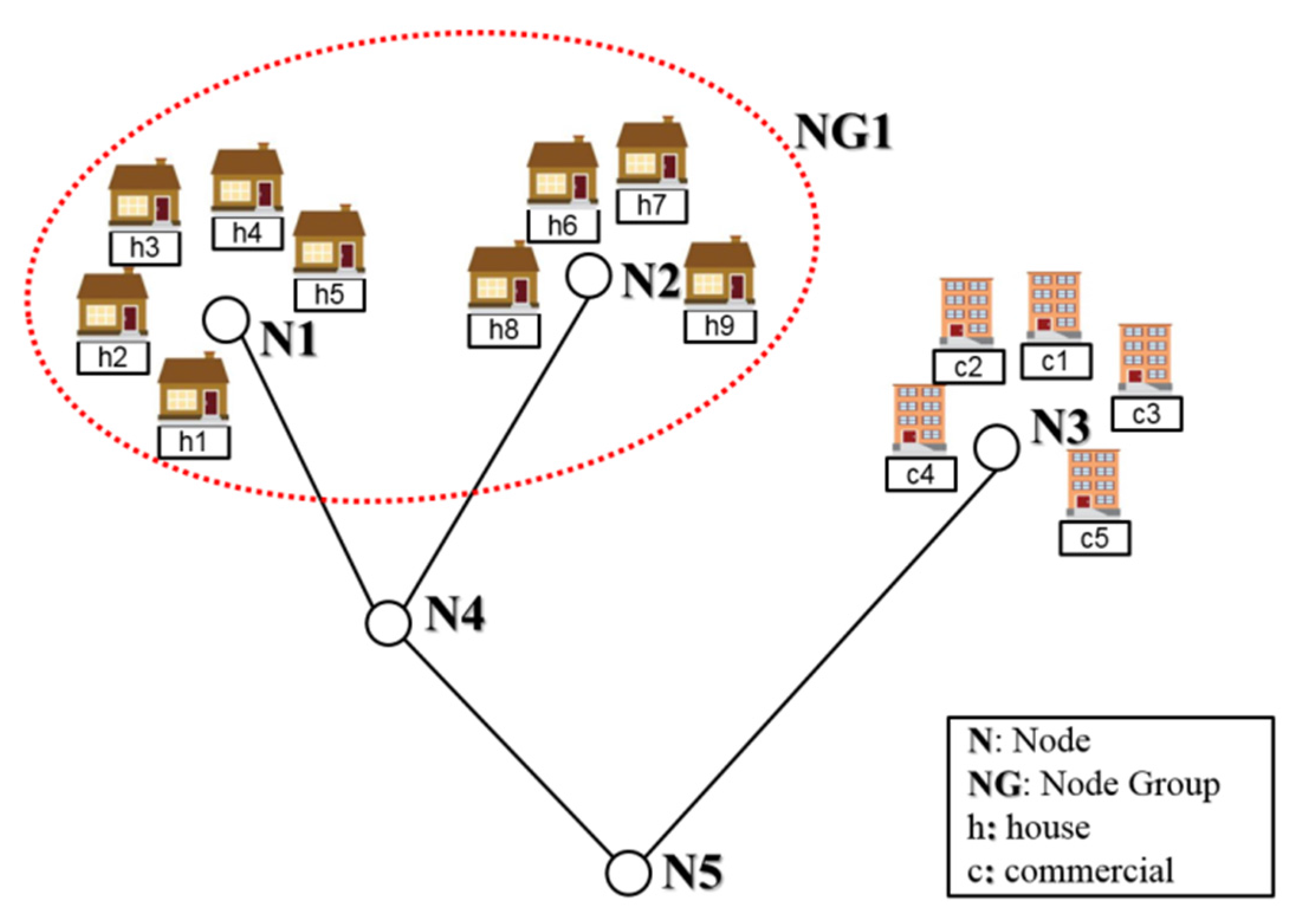
A water distribution system (WDS) comprises various components (e.g., nodes, pipes and pumps), each of which has its own purpose and function. For example, a pumping unit elevates the total head of water to supply demand at high elevation, whereas a pipe transports water from one location to another. Hydraulic WDS models have been developed for many reasons, including design and rehabilitation, operation and management and system surveillance. The real-world system is simplified for modeling purposes during the development process of a hydraulic model. As shown in Figure 1, a group of households (h1–h5) can be simplified to node N1, because they are the same type of users (i.e., residential) and in proximity to each other. Similarly, households h6–h9 can be modeled as node N2. Node N3 is the sum of the commercial demands c1–c5.

State estimation is defined as the process of calculating a state variable of interest that cannot be directly measured [1,2]. In a WDS, nodal demands are often considered as state variables (i.e., unknown variables) and can be estimated using nodal pressures and pipe flow rates measured in the field. Previous demand forecasting/estimation studies have focused on estimating hourly to monthly macro-scale demand (i.e., total system demand) by using time series models [3,4,5,6]. A few studies have recently proposed micro-scale demand (i.e., nodal demands) estimation methodologies with a more precise time step (e.g., 15 min) based on coupling the Kalman filter (KF) with a hydraulic simulator (e.g., EPANET [7]) [2,8]. Advances in sensor technology, such as increased battery lifetime and communication frequency, have encouraged the development of demand estimation techniques compatible with field measurements from advanced sensors (e.g., advanced metering infrastructure (AMI)).

The WDS demand estimation can produce accurate results when sufficient field measurements are available. However, a sufficient number of meters cannot be installed in a system because of budget constraints. In demand estimation, the demand is the unknown variable, whereas the pipe flow/nodal pressure is the known variable. Therefore, the number of unknowns should be reduced to make the demand estimation problem even-determined. An alternative is to aggregate (i.e., group) the nodes. For example, nodes N1 and N2 can be aggregated to Node Group 1 (NG1) because they have the same residential usage pattern (Figure 1).

Many methodologies have been proposed for the WDS component grouping, clustering and aggregation in the last two decades. However, most do not target demand estimation. Mallick et al. [9] investigated the tradeoff between the WDS model error caused by simplification (i.e., pipe grouping) and the model prediction error. They subsequently proposed a method to identify the best number of pipe groups. Deuerlein [10] proposed a water distribution network decomposition method that classifies network components into forest, bridge and biconnected-block components. The latter two are called “core components”. The three component types are used to augment the network graph. Perelman and Ostfeld [11] developed a multilayered clustering method as an extension of their previous clustering algorithm [12] based on depth-first search [13] and breadth-first search [14].

Diao et al. [15] proposed a community structure identifier that uses modularity (M) as an indicator to “quantify the quality of the graph division into communities” [16]. This approach merges vertices so that communities are aggregated with the greatest increment of modularity (ΔM). In their follow-up paper [17], they proposed a methodology to decompose a WDS into a twin-simplified pipeline structure comprising backbone mains and community feedlines.

Di Nardo et al. [18] used graph theory principles and a heuristic procedure for WDS sectorization based on minimizing the amount of dissipated power in a WDS. Giustolisi and Ridolfi [19] developed a multi-objective strategy for optimal WDS segmentation that maximizes a modified modularity index and minimizes the cost of newly-installed devices to obtain network segments. In summary, little effort has been devoted to the application of an optimization technique to the WDS component grouping, clustering and aggregation.

Few studies have considered node grouping as a method of decreasing the unknown dimensions for the WDS demand estimation. Kang and Lansey [2] compared the two following real-time demand estimation methods with respect to their WDS demand estimation accuracy: the tracking state estimator and the KF. They aggregated nodes in a study network into multiple groups to reduce the number of unknowns and to make the demand estimation problem overdetermined or even-determined, which was also suggested in [20]. Jung and Lansey [8] employed the nodal demand aggregation approach of Kang and Lansey in their KF-based WDS pipe burst detection model. They then demonstrated that using the same number of node groups as the number of flowmeters yielded the best accuracy with the KF-based demand estimation scheme.

Note that the KF-based estimation method has been used for real-time WDS demand estimation [2,8], whereas optimization techniques have been widely used for demand and its hourly pattern calibration, which estimates base demands and leakage (non-real-time estimation) [21,22,23,24]. Less estimation time is generally allowed for the former (e.g., 5 min), which results in using different methodologies for the two different estimation purposes. The base demand and its hourly pattern are not to be determined in the real-time demand estimation. The commonality is in the use of a hydraulic model (e.g., EPANET). Accordingly, the demand calibration methodologies solve a non-linear system equation to quantify the accuracy of possible solutions, whereas the KF-based method solves a network equation to obtain pipe flow rates compared to field measurements.

Node grouping is one of the most important factors affecting the accuracy of the WDS demand estimation. However, previous studies have determined node groups based on engineering knowledge/sense (e.g., grouping nodes with the same demand pattern or in proximity) or assumed that they are given. Identifying optimal node groups using such approaches is very difficult considering the complex hydraulic relationship between the pipe flows/nodal pressure at sensor locations and the demand of node groups, especially in actual large networks (mostly loop-dominated). Note that the task is more difficult when sensors are not located at the best points for demand estimation, which is generally not the main concern during the sensor network design. Therefore, an optimization-based approach to find the optimal node groups for a highly accurate WDS demand estimation is required.

This study proposes an optimal node grouping (ONG) model to maximize the accuracy of the real-time WDS demand estimation. The KF-based demand estimation method is linked with a genetic algorithm (GA) for node group optimization. The modified Austin network demand is estimated to demonstrate the proposed model’s validity. True demands and field measurements are synthetically generated using a hydraulic model of the study network.

2. Methodology

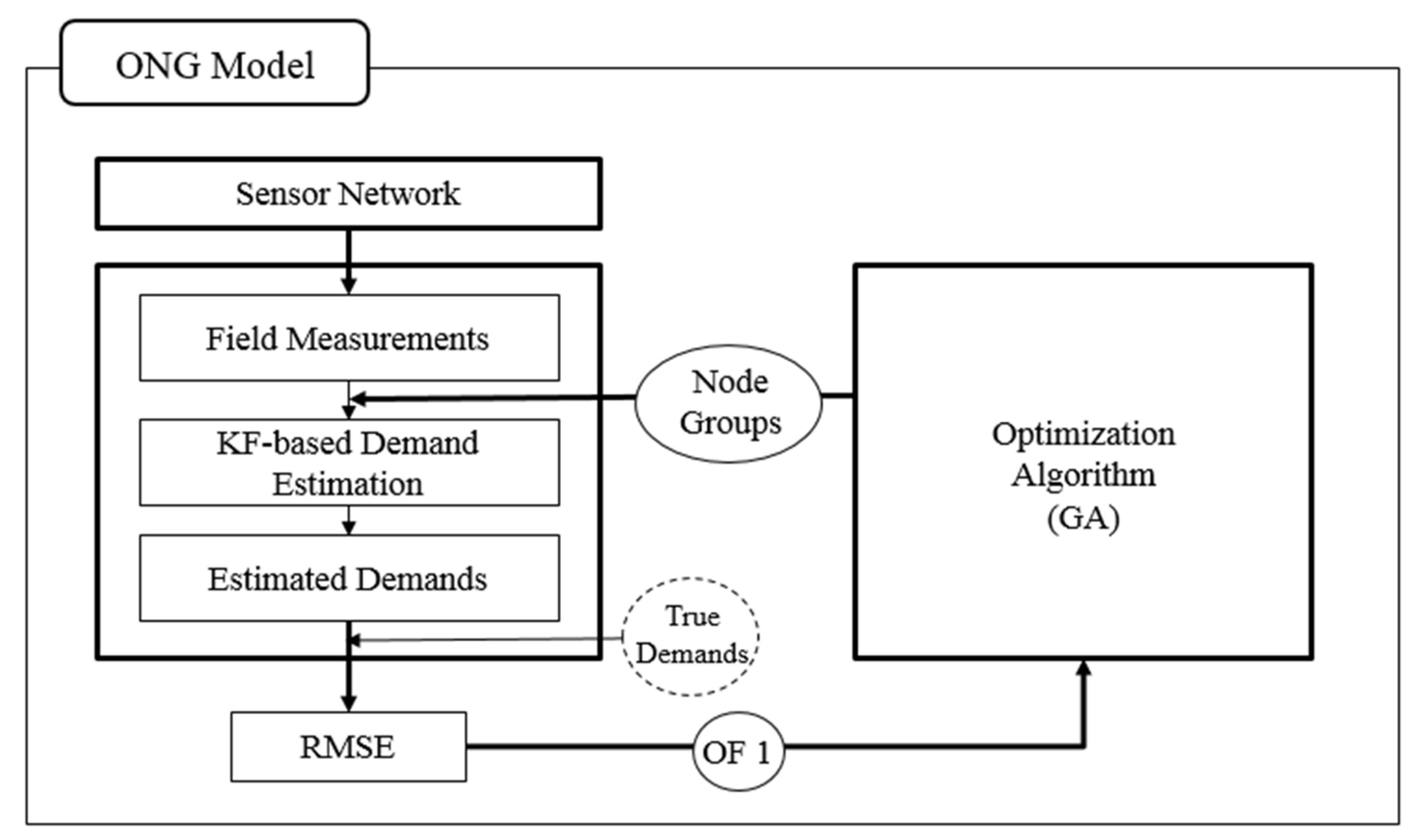
This research proposes an ONG approach that minimizes the sum of the root-mean-square error (RMSE) for the estimated demands of a given number of node groups. The nodes should be aggregated to decrease the number of unknowns in the demand estimation problem. Figure 2 shows the structure of the proposed ONG model, which comprises three main submodules. Each submodule represents an important factor that affects the demand estimation accuracy.

The WDS demand estimation accuracy is affected by the available information, estimation method and node grouping. The amount of information from field measurements on the estimated demand is a function of the number and types of sensors and their locations. The sensor network layout (i.e., number and location of sensors) is assumed to be provided (“sensor network” in Figure 2) because the demand estimation is not a primary concern for decisions on the number and type of sensors and their locations. The KF-based WDS demand estimation methodology proposed by Jung and Lansey [8] is employed in this study because of its high accuracy. Based on the potential node groupings provided from the optimization algorithm (GA) submodule and field measurements obtained from the sensor network, the KF-based method estimates the node group demands. The accuracy is then quantified using the RMSE. The RMSE serves as the fitness value of the node grouping optimization and is minimized to increase the WDS demand estimation accuracy.

The following subsections detail the node aggregation, field measurements, KF-based demand estimation method, ONG model and GA. The blocks corresponding to each subsection are shown in Figure 2.

2.1. Node Groups and Demand Patterns

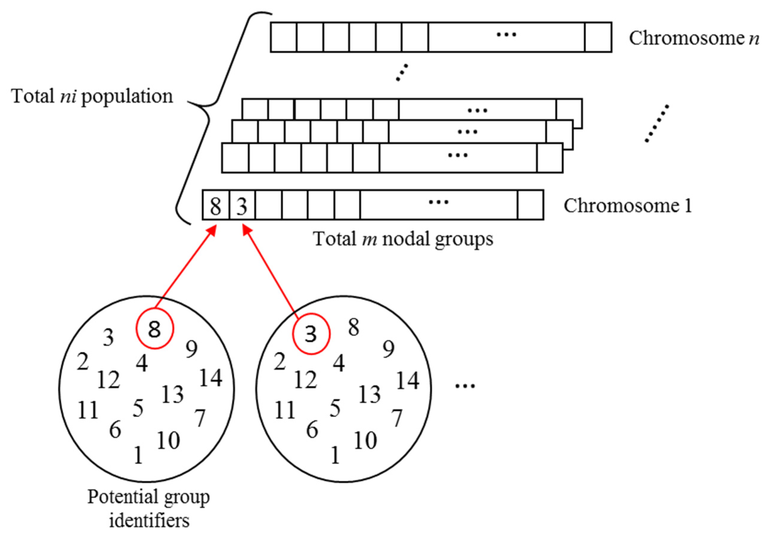
Each node can be classified into one of the node groups. However, the total number of groups is predefined. Each node is labeled with an integer number from 1 to the total number of node groups during optimization. For example, each node is indexed among integers 1–14 if the WDS has a total of 14 node groups. This number is set equal to the total number of flowmeters. Therefore, the decision variables of the proposed ONG problem are all integer values (Figure 3).

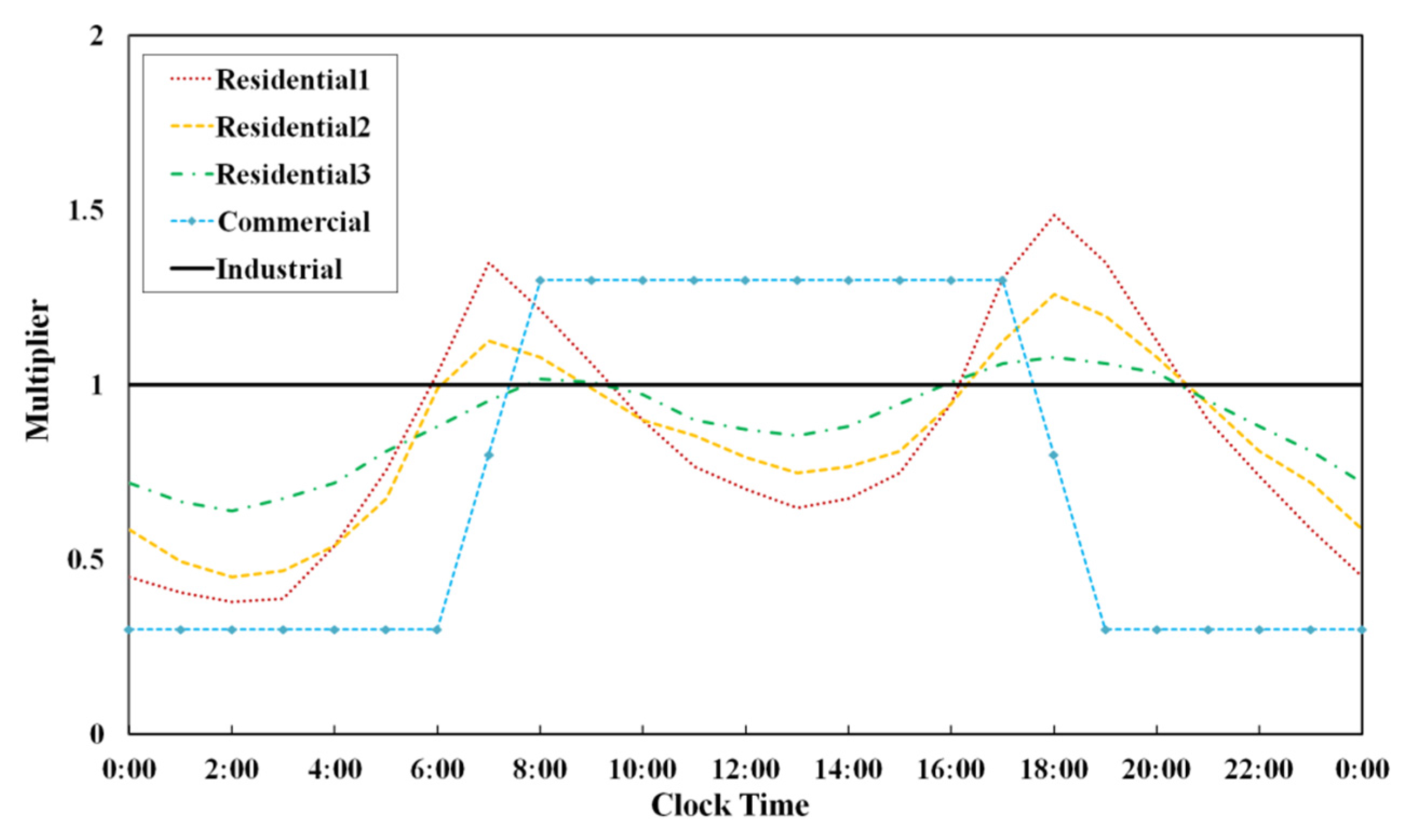
Figure 4 shows the five following general diurnal demand patterns considered by Kang and Lansey [2]: three residential, one industrial and one commercial. The three residential users are an apartment (Residential 1 in Figure 4), houses with half-acre lots and large home lots (Residential 2 and 3, respectively). The residential apartment demand is characterized by higher peaks early in the morning (6–7 a.m.) and evening (6–7 p.m.) than those of the other two residential demands. Note that a residential user with a large lot has the lowest peak factor and attenuated demand change during the day. The industrial water usage is relatively constant throughout the day, while the commercial demand sharply rises and falls at the start and end of the workday and is constant during the workday.

All users are assumed to be in apartments (Residential 1), which is easily valid for highly dense urban areas. More complicated demand estimation problems can be formulated by randomly setting the user type for a node from the above five types, assuming that there is no spatial correlation in the demand patterns. However, this is not realistic. In the real world, demand patterns show strong spatial correlations (e.g., commercial districts are in the downtown area of a city).

2.2. Field Measurements

The KF-based demand estimation method estimates real-time node group demands using field measurements (e.g., pipe flow rate and nodal pressure) received from a supervisory control and data acquisition system. The pipe flow rate and nodal pressure are the output variables, whereas the node group demands are the input variable of the WDS. Note that the nodal demands can easily be calculated from the node group demands. Therefore, the KF-based method reverse-engineers the input variable, which cannot be directly measured, using the output variables, which can be measured by meters installed throughout the system.

In this study, the field datasets of the pipe flow rate are synthetically generated to assess the accuracy of the KF-based demand estimation method given the potential node groupings (Figure 2). The field measurements for the nodal pressure are assumed to not be utilized for the WDS demand estimation because low accuracy is observed when nodal pressure measurements are included [8].

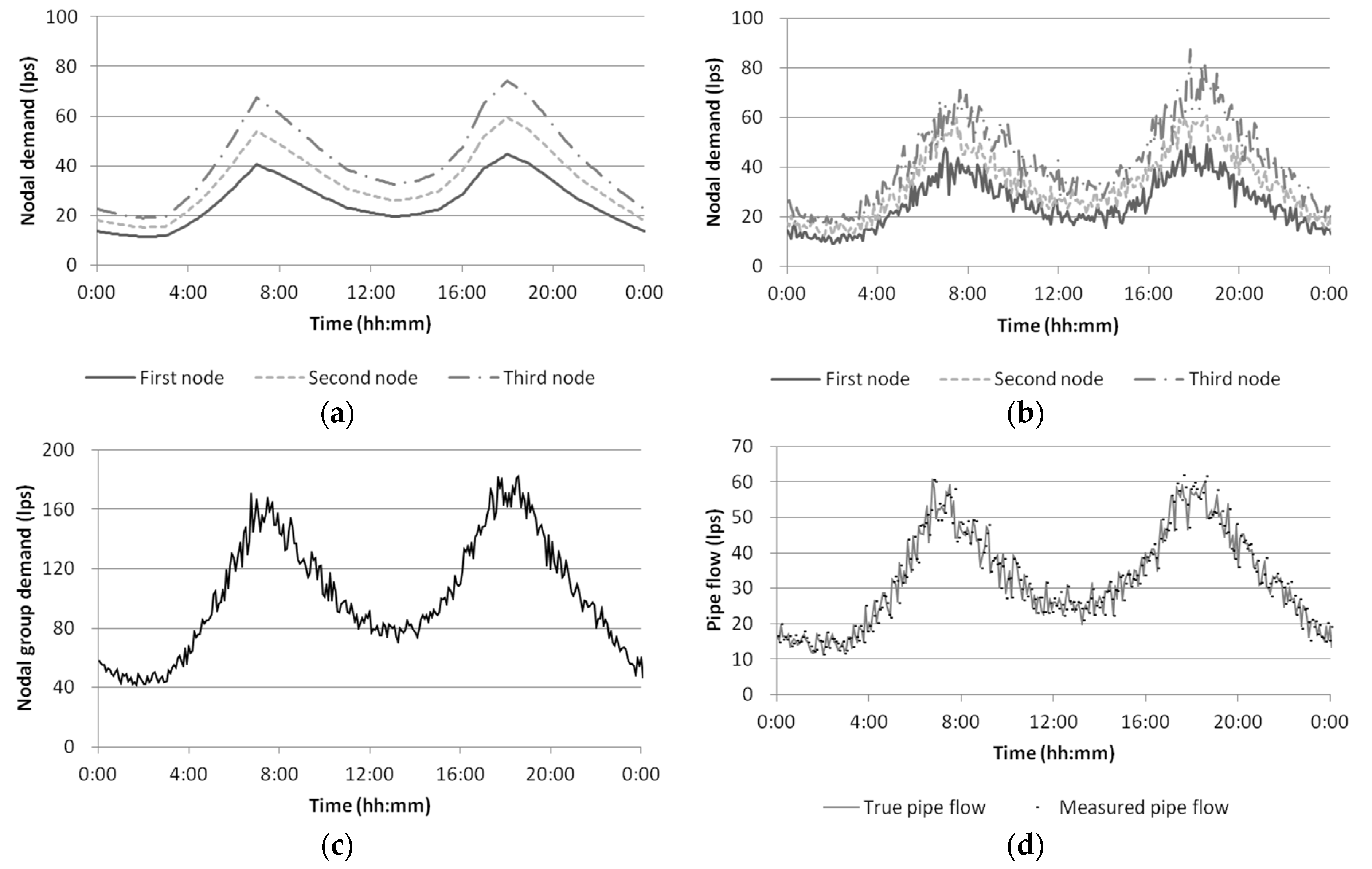
The synthetic pipe flow rates are generated following these procedures: (1) an identical demand pattern (Residential 1 in Figure 4) is assigned to each node in the system (Figure 5a); (2) random deviations $N\left(0,{\sigma }_q\right)$ (i.e., white noise) are added to each demand to consider the randomness and heterogeneous nature of true nodal demands (Figure 5b); (3) true node group demands are calculated by summing the demand of nodes in a group (Figure 5c); (4) the nodal demands generated in Step (2) are entered into an EPANET hydraulic model of the study network to generate true pipe flow rates; and (5) another white noise is added to each pipe flow rate to introduce measurement errors $N\left(0,{\sigma }_Q\right)$ (Figure 5d).

While the assumption of the normal distribution for the nodal demand is common in WDS design [8,25,26], Surendran and Tota-Maharaj [27] have recently confirmed that normal and lognormal distributions are appropriate for WDS demand based on analyzing real daily water consumption data with a 15-min interval for four years in the U.K. Auto-correlated noise (e.g., a sports event lasting for 2 h) can be considered for Step (2) to simulate more realistic demand fluctuations [28,29]. Note that the effect of considering different noise types on the accuracy of the KF-based demand estimation method would be minimal because it estimates the state variable, such that the error covariance is minimized.

2.3. KF-Based Demand Estimation

The KF-based demand estimation method links the field measurements with the hydraulic simulation model (EPANET) that solves the non-linear system equation comprising mass and energy conservations [2]. Before demand estimation, the nodes are grouped into a single demand (i.e., nodal group demand) following the grouping from the optimization submodule (Figure 2) to overcome the limitation of low measurement redundancy. The field pipe flow data are measured in real time. First, aggregated demands are estimated using the final demand estimates of the previous time step. The estimated group demands are disaggregated to individual nodes, which are entered into the hydraulic simulation model to calculate the pipe flow rate estimates. The demand estimates are updated such that the error covariance is minimized using the gap between the field measurement and the estimate of the pipe flow rate.

The KF comprises the recursive implementation of forecast and update steps, such that the a posteriori error covariance is minimized. The forecast step estimates the state at the current time step using the state estimate from the previous time step. The update step refines the forecast based on measurements at the current time step for a more accurate state estimate in the current time step. When calculating the state estimate in the update stage, more weight is given to the state estimate with the smaller uncertainty between those from the forecast stage and those from the current measurement [30].

The KF has the advantage of embedding the system dynamics in the estimates, which enables it to consider system operational changes when estimating the demand for a set of nodes (node group demands) based on the measured pipe flows.

The two types of KF are linear (LKF) and non-linear (NKF). The NKF represents the full non-linear relationship between measurements and states, whereas the LKF employs the linearization of these functions. The NKF is used herein because of its higher accuracy for the state estimation of a WDS (i.e., a non-linear system) than the LKF [8].

The state forecast $x_k^{-}$ (i.e., the a priori state estimate of the node group demands) is computed using the state equation as follows:

$$x_k^{-}=A_k{x}_{k-1}^{+}+w_k,w_k~N\left[0,Q_k\right]$$

(1)

where A_k relates the state at the previous time step k − 1 to the state at the current step k. This matrix is updated at each time step and calculated from the historical mean node group demand values; w_k is a random variable representing the process noise; and Q_k is the process noise covariance. Note that node grouping is provided from the optimization algorithm submodule (Figure 2) based on the methodology described in Section 2.1.

In the NKF, the non-linear system function h in the measurement equation relates the a priori state estimate ($x_k^{-}$) and exogenous variable (u_k, operational information) to the measurements (pipe flows) as follows:

$$z_k=h\left(x_k^{-},u_k\right)+v_k,v_k~N\left[0,R_k\right]$$

(2)

where z_k denotes the measurement variables; v_k is a random variable representing the measurement noise; and R_k is the measurement noise covariance.

The updated state estimate (i.e., the a posteriori state estimate of the demand) is given as:

$$x_k^{+}=x_k^{-}+K_k\left(z_k-h\left(x_k^{-},u_k\right)\right)$$

(3)

where K_k is the Kalman gain matrix expressed as follows:

$$K_k=P_k^{-}{H}_{uk}^T{\left(H_{uk}{P}_k^{-}{H}_{uk}^T+R_k\right)}^{-1}$$

(4)

where H_uk is the Jacobian matrix of the partial derivatives of h with respect to x and u, and a unique H_uk is computed for each system operational state (u_k) around the a priori state estimate $x_k^{-}$; and $P_k^{-}$ is the a priori estimate error covariance calculated as follows:

$$P_k^{-}=A_k{P}_{k-1}^{+}{A}_k^T+Q_k$$

(5)

Therefore, the a posteriori state estimate $x_k^{+}$ is computed as a linear combination of the a priori estimate $x_{\mathrm{k}}^{-}$ and the weighted difference between the actual z_k and predicted $h\left(x_k^{-},u_k\right)$ measurements. For example, a large measurement error covariance R_k results in a small update correction to the forecast state vector $x_k^{-}$.

The a posteriori estimate error covariance is finally calculated as follows:

$$P_k^{+}=\left(I-K_k{H}_{uk}\right)P_k^{-}$$

(6)

The LKF uses the linear transition matrix H in Equations 2 ($z_k=H{x}_k^{-}+v_k$) and 3 ($x_k^{+}=x_k^{-}+K_k\left(z_k-H{x}_k^{-}\right)$). The LKF can be used for non-linear systems h(x) with weak non-linearity, but may perform poorly as the non-linearities increase. Both the LKF and NKF use first-order approximations for the error covariance propagation ($H_{uk}{P}_k^{-}{H}_{uk}^T$ in Equation 4 and $A_k{P}_{k-1}^{+}{A}_k^T$ in Equation 5). A perturbation method, wherein the derivatives are approximated by the numerical forward finite differences, is used to calculate H_uk.

Note that a KF is classified as linear or non-linear based on the type of underlying state and measurement equation and not on the first-order approximation. The extended KF can only be applied to an NKF that estimates $w_k$ and $v_k$ in Equations 1 and 2, respectively, along with the state.

2.4. Demand Estimation Accuracy Indicator: RMSE

The state estimate includes errors because of measurement and model errors and the state variable randomness. Measurement errors can originate from deterioration and imperfect calibration of meters and delays in data communication (e.g., missing data). Model errors originate from model parameter uncertainties and a lack of system knowledge (e.g., erroneous system structure). This study aims to find the optimal node grouping that minimizes the model errors when estimating the WDS node group demands. The RMSE is used as an indicator of the WDS demand estimation accuracy (Figure 2). The RMSE measures the difference between values predicted by a model or estimator (KF) and the true values and is calculated as follows:

$$RMSE=\sqrt{\frac{{{\displaystyle \sum }}_{k=1}^{nt}{\left(E_k-O_k\right)}^2}{nt}}$$

(7)

where nt is the total number of time steps; E_k is the estimated group demand at time step k (obtained from the KF-based demand estimation method described in Section 2.3); and O_k is the true group demand at the k-th time step (synthetic measurements are obtained by the methodology described in Section 2.2).

2.5. Elitism-Based GA

A GA [31] is a metaheuristic optimization algorithm that mimics the process of natural selection (i.e., “the survival of the fittest”). A standard GA (SGA) generally begins with a randomly-generated initial population (i.e., group of potential solutions). A pair of solutions is selected with a high probability to have high fitness (selection process), which is then subjected to crossover and mutation processes that share their genetic traits (i.e., decision variables) and modify a few of them, respectively. This series of processes (selection–crossover–mutation) is called an “iteration.” This series is continued until the child population is filled. Better fitness solutions tend to appear in the population over iterations.

Various versions of the GA have been released after Holland [31] first introduced the SGA. These versions include the elitism GA, greedy GA, adaptive GA and refined GA [32,33,34,35]. One of the reasons for such a massive number of releases is that SGA is not capable of keeping the current best solution for the next generation. In other words, SGA is inefficient at considering new and good solutions found in the iterations. Therefore, an elitism-based GA (eGA) is proposed to optimize the WDS node grouping problem.

The proposed eGA selects two solutions from the parent population through roulette wheel selection, where the probability of a solution to be selected is proportional to its fitness. Similar to the general GA, a high fitness solution has a better chance to be selected. The general crossover and mutation processes are then performed at frequencies defined by the crossover and mutation rates. Crossover generally occurs with a probability of 70%–90%, while mutation happens with a probability of 2%–10%. The resulting two solutions are called children solutions. The two new children solutions compete with the selected parent solutions in a tournament with respect to fitness to determine whether any of the two children solutions can replace the parent solution(s). Therefore, one iteration of eGA requires only two functional evaluations, whereas the SGA requires ni number of functional evaluations, where ni is the total number of individuals (i.e., solutions) in the population. The prompt inclusion of newly-found good solutions in the eGA improves the search efficiency of the SGA because the solution can be considered as a parent solution for selection in the immediately following iteration. Chromosomes are integer-coded (i.e., decision variables are in integers) in the eGA (Figure 3) for the node grouping optimization in the WDS demand estimation.

2.6. Optimal Node Grouping Model

While the number of unknown variables (i.e., demands) should be reduced because of the lack of available information, an accurate demand estimation can be achieved when each pipe flowmeter is linked to an appropriate node group, which is usually the group of nodes in proximity to the meter, whose demand affects the pipe flow rate. Therefore, given the layout of pipe flowmeters, finding the optimal node groups plays a very important role in determining the WDS demand estimation accuracy. Provided that there is no spatial proximity information between the meters and the nodes, the proposed optimal node group model finds the optimal node groups that minimize the total RMSE of the estimated node group demand using the KF-based method given the total number of node groups:

$$\text{Minimize }F={\displaystyle \sum }_{i=1}^{ng}RMS{E}_i$$

(8)

$$\text{subject to }ng=m$$

(9)

where RMSE_i is the RMSE of the i-th node group; ng is the total number of node groups (i = 1, 2, ..., ng); and m is the total number of node groups predefined by the user generally equal to the total number of pipe flowmeters in the WDS.

Note that pressure constraints are not included in the proposed ONG problem, which differs from other optimization problems (e.g., WDS design problem) developed in the WDS field. However, the synthetic demand generated by the methodologies described in Section 2.1 and Section 2.2 results in nodal pressures in a normal operation range of 21–28 m (30–40 psi).

3. Application

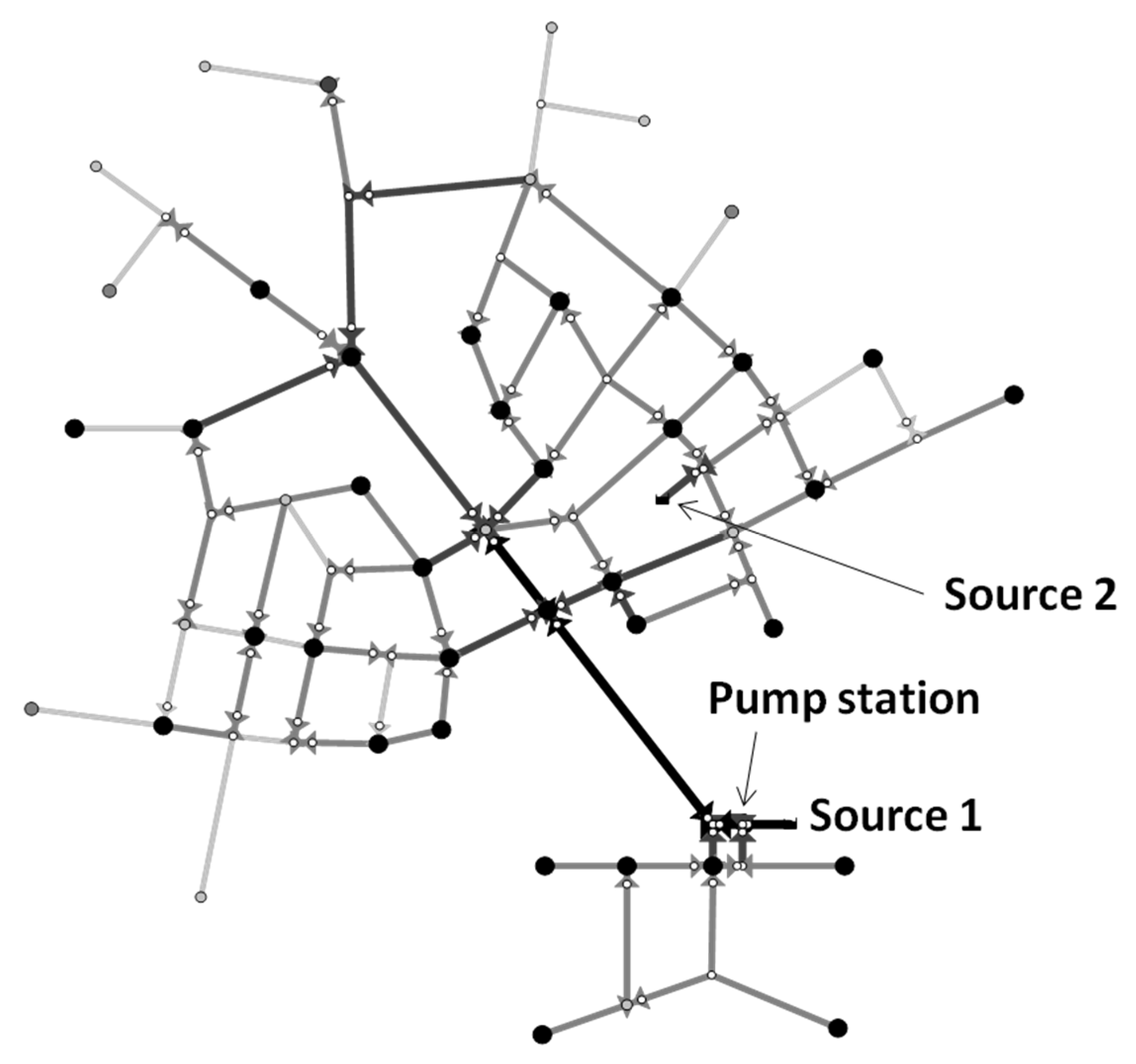
The proposed ONG model is applied to estimate the Austin network demand [36] with modifications [8]. The Austin network is a non-district metering area (DMA) structured loop-dominated network. As shown in Figure 6, the modified system comprises 126 nodes and 90 pipes supplied by two reservoirs and one pumping station. Similar to the original network, the modified Austin network is solely supplied by a single reservoir (Source 1) with a fixed source head (306 m). The second reservoir (total head = 366 m) in the middle of the loop in the east corner of the system is not operated.

Only 47 nodes have external demands. Therefore, the total number of unknown demand nodes is 47. The rest of the nodes (i.e., 79 nodes) are pipe connections with no external demands. A total of 14 pipe flowmeters are assumed to be installed throughout the system. The meters are assumed to be installed at the same locations selected by Jung and Lansey [8]. The number of node groups is set equal to the number of meters to realize high demand estimation accuracy. Therefore, the 47 demand nodes are assumed to be aggregated into 14 node groups (i.e., m = 14).

A two-day series of node group demands and pipe flow rates is generated at 5-min time steps using the network’s hydraulic model based on the methodologies described in Section 2.1 and Section 2.2. Similar to Jung and Lansey [8], the Kang and Lansey approach [2] is applied to demand aggregation and disaggregation. The method is briefly described here. The forecast node group demands at the current time (aggregated demands) are estimated from the transition of the updated demand of the previous time step (Equation (1)). The forecast node group demands are then disaggregated to individual nodes under the assumption that the nodal demands (disaggregated demands) in the same group are perfectly correlated. During the disaggregation, the ratio of the individual nodes’ base demands to the total node group base demand is multiplied by the forecast node group demands to obtain the individual nodal demands.

The demands are normally distributed with a coefficient of variation (CV) of 0.1 (${\sigma }_q=0.1{\mu }_q$). The measurement errors are random variables $N(0,\sigma$), where ${\sigma }_Q=0.1{\mu }_Q/3.27$ (corresponding to a measurement error of 10%) for pipe flow measurements. All nodes are considered to be residential users in apartments.

eGA is used to find an optimal solution for the ONG problem, wherein the number of possible solutions is 7.379 × 10⁵³ (= 14⁴⁷). Note that the well-known Hanoi network design problem has 2.865 × 10²⁶ (6³⁴) possible solutions [37]. The crossover and mutation processes are conducted with probabilities of 85% and 5%, respectively. The genetic traits of the chromosomes are shared at multiple scattered points, while the standard mutation is employed. The node grouping determined by the engineering decision of Jung and Lansey [8] (i.e., a node group comprising nodes of the same user type) is seeded as an initial solution, whereas the other initial solutions, where the population is 100 (ni = 100), are randomly generated by uniform sampling among 1–14 integer values. The eGA returns the best solution when the solution is not changed over 300 iterations.

4. Application Results

The KF-based method was used to consider a two-day series of pipe flow rates measured at 14 meter locations for node group demand estimation. The RMSE for each group (Equation (7)) were calculated by comparing the synthetically-generated node group demands for two days (both the pipe flow rates and node group demands were in 5-min time steps) with the estimated values. The erroneous node groups resulted in the divergence of the state estimates, which mostly originated from a badly-scaled or (nearly) singular matrix in Equation (4) (i.e., the determinant of the matrix ($H_{uk}{P}_k^{-}{H}_{uk}^T+R_k$) to be inversed was close to zero). In the optimization of the proposed ONG model, a high penalty value (e.g., 10,000 × 14 = 140,000) was added to the objective function value (i.e., RMSE) in Equation 8 if a matrix was ill-conditioned. The demand estimation was terminated at the time step to speed up the optimization when the ill-conditioned matrix was identified.

Note that the KF-based demand estimation method estimated the nodal group demands only using pipe flow measurements without being given any information/values of the true nodal group demands. In this study, the true nodal (group) demands were synthetically generated and entered into the WDS system equations to obtain pipe flow rates at locations, to which the measurement error was added to finally produce the pipe flow measurements. Processed using the non-linear governing equations and added noises, the pipe flow measurements did not contain clear clues for tracking the true nodal group demands. Therefore, estimating the nodal group demands was not a circular numerical calculation.

First, the differences between the node groupings of the initial and final optimal solutions were investigated. Then, the spatial distributions of the nodes in a group and node groups were examined along with whether or not there was a one-to-one relationship between a meter and a node group. The RMSE values of the individual node group demand estimates were determined. Conclusions were drawn on the demand estimation error, base demand of the node group and meter locations.

4.1. Optimal Node Grouping Results

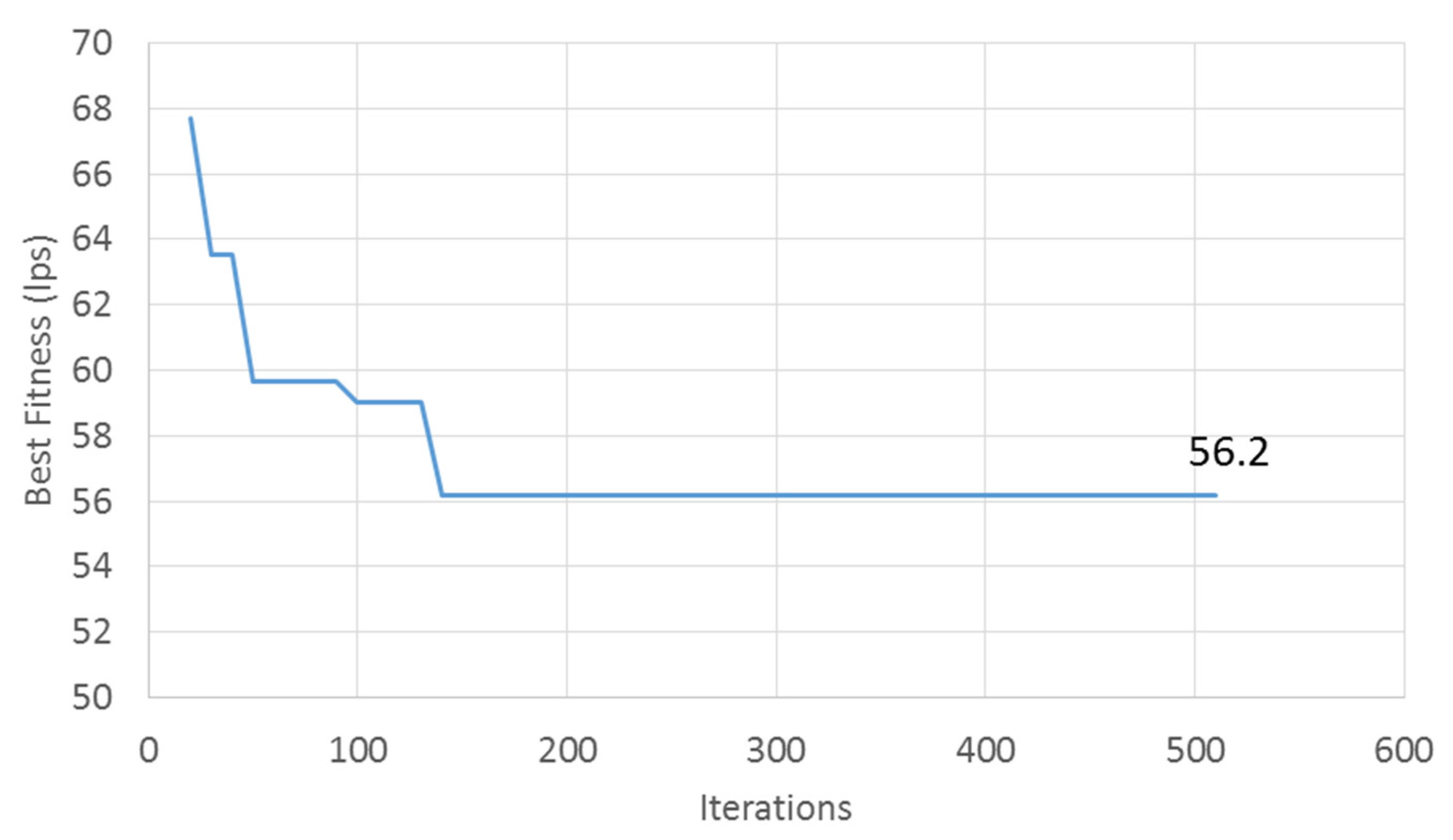
Figure 7 shows the trajectory of the best fitness value (i.e., sum of node group RMSEs) over the iterations. Note that the sum of the RMSEs reported by Jung and Lansey [8] was 74.1 L/s. They determined the node grouping based on engineering judgment. The best RMSE with the proposed ONG model was 56.2 L/s, which was about 76% of the RMSE obtained by Jung and Lansey [8] (Figure 7). Jung and Lansey [8] included seven nodes (out of 47 demand nodes) with industrial and commercial demands, which slightly complicated their demand estimation. Other conditions (e.g., meter locations and measurement time interval) were the same as in this study.

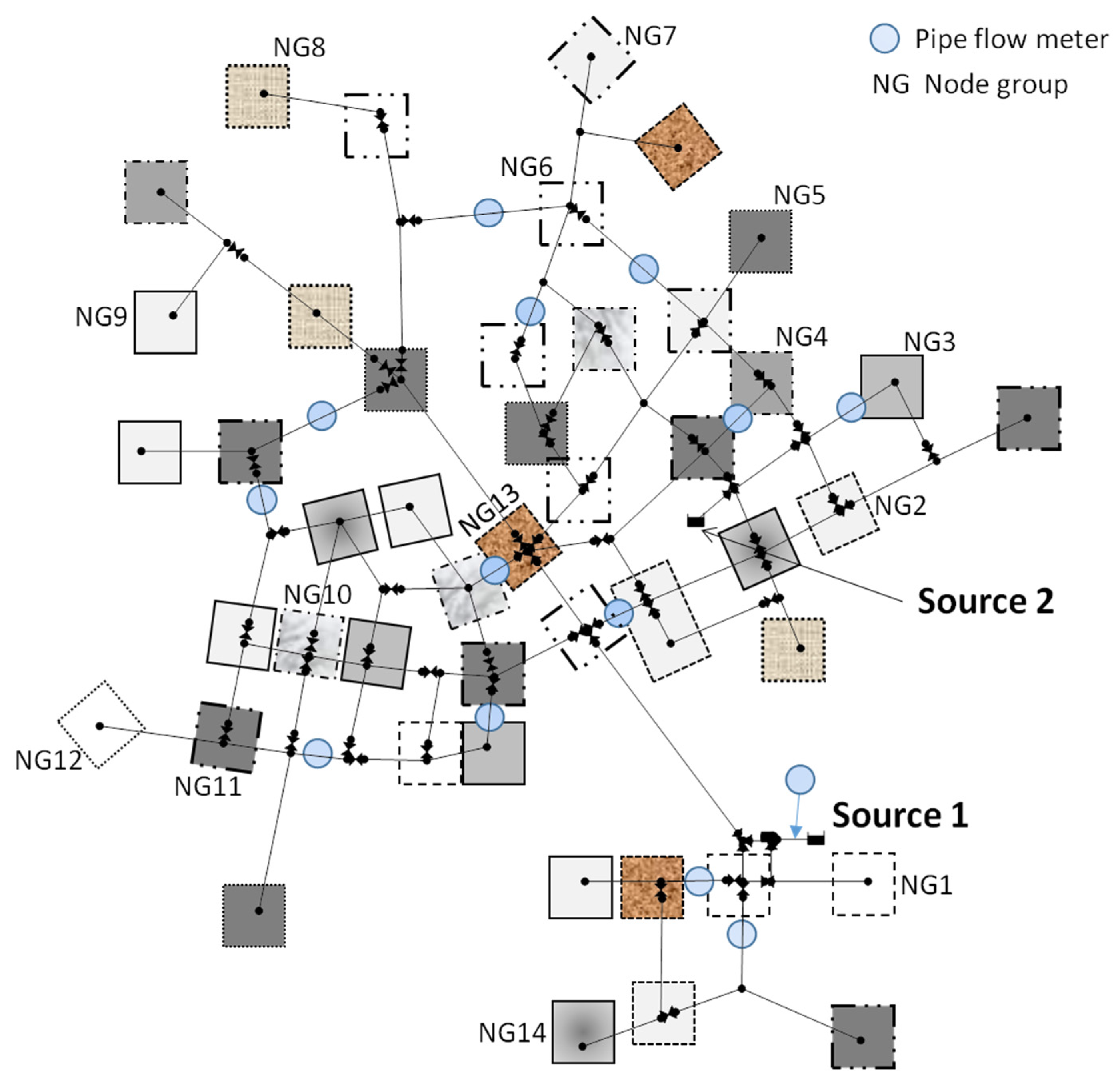
Most solutions found in the early stage of the optimization had diverging demand estimates (i.e., infeasible solutions with a penalty value), which resulted in the solution’s fitness value of 140,000 (not included in Figure 7). The main reason for the divergence was the scattered distribution of node groups (Figure 8). Generally, the highest accuracy is achieved when a group of gathered nodes had a one-to-one relationship with a meter in close proximity (opposite condition to the node grouping in the infeasible solutions). A feasible solution was found after a few iterations, and step decreases in the fitness value were observed until the best fitness was reached at the optimal value of 56.2 L/s. The results for the individual node group demands were discussed in Section 4.2.

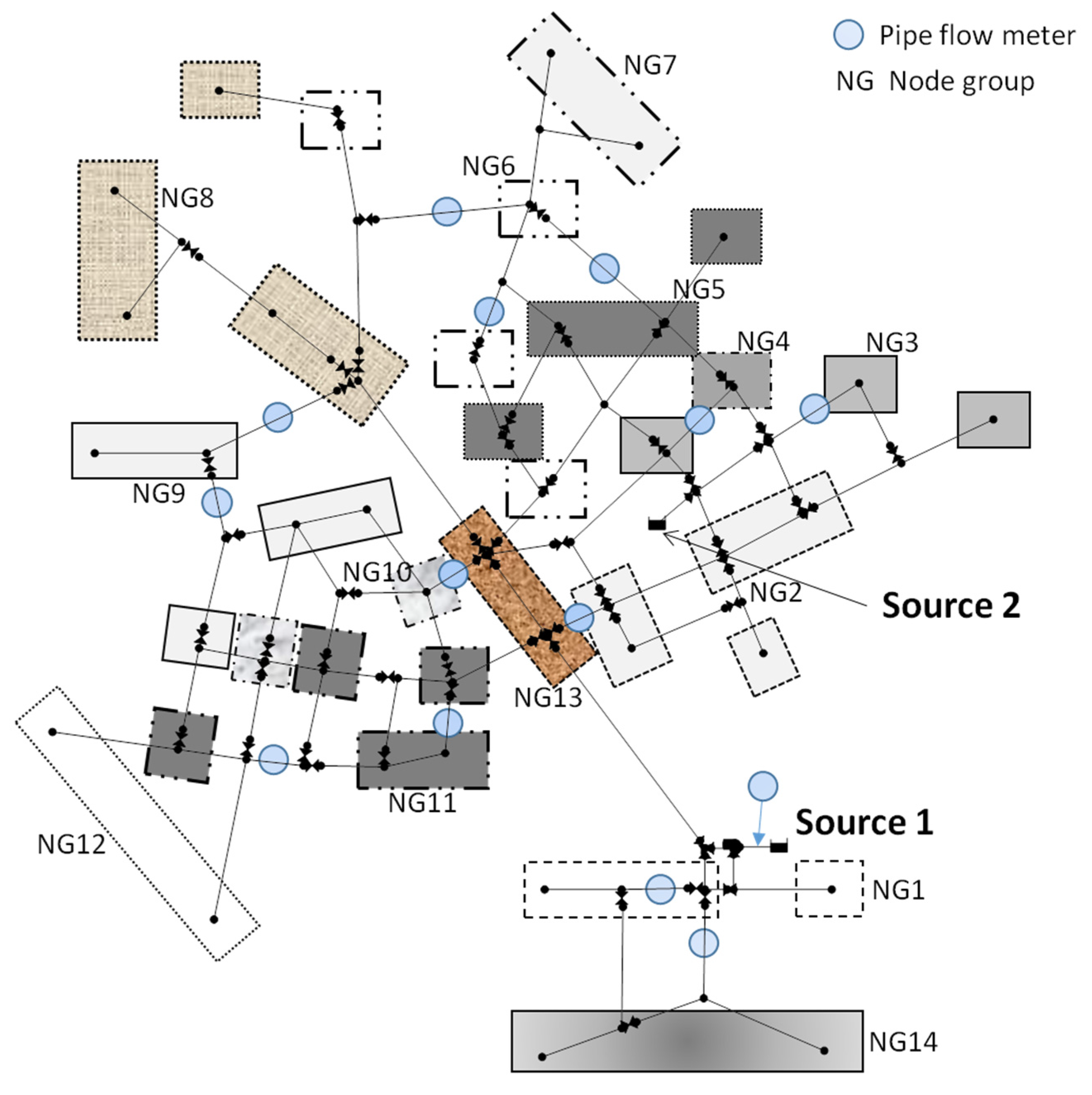
Figure 9 shows the optimal node grouping layout found by the proposed node grouping model. In contrast to the representative initial solution shown in Figure 8, the optimal solution spatially gathered nodes in each group. For example, Node Group (NG) 14 comprised three nodes in proximity at the south end of the study network, whereas the five nodes at the north end composed NG8. NG4 only had one node. Some node groups (e.g., NG3, NG6 and N10) comprised nodes that were not close to each other (i.e., slightly scattered), which was mostly caused by the existence of node(s) with no external demand between the nodes. For example, there was a zero-demand node between the leftmost and middle nodes in NG3. In addition, the three zero-demand nodes near NG11 were also worthy of being seen (Figure 9).

Figure 9 also shows the location of the 14 meters installed in the study network. Note that not only was a meter located at the transmission mains (e.g., the source pipe linked to Source 1 and two pipes on the right and left sides of the NG13 box), but one was also installed in the distribution pipes within the loops at the northeast and southwest parts of the network. Finding an apparent one-to-one relationship between a node group and a meter was very difficult because of the complex hydraulic relationship of a looped network. Compared to a simple branched network, the response of the pipe flow rate at the meter location to a perturbation in the node group demand, which was information required for demand estimation, cannot be easily identified by visual inspection or engineering knowledge/sense in a looped network. Therefore, this result highlighted the need for the proposed model when trying to find optimal node groups that result in a highly accurate WDS demand estimation.

Multiple optimal (or near-optimal) solutions for the ONG problem of real large networks could be employed. More preference would be given to the solution with a high tendency of classifying nodes in proximity or of the same user type into the same group.

4.2. Accuracy of Individual Nodal Group Demand Estimation

Table 1. Node group demand estimation RMSE (sum of node group demands’ RMSE = 56.2 L/s).

Node Group (NG)	1	2	3	4	5	6	7
RMSE (L/s)	7.7	4.9	2.4	1.8	4.4	2.0	1.2
Node group (NG)	8	9	10	11	12	13	14
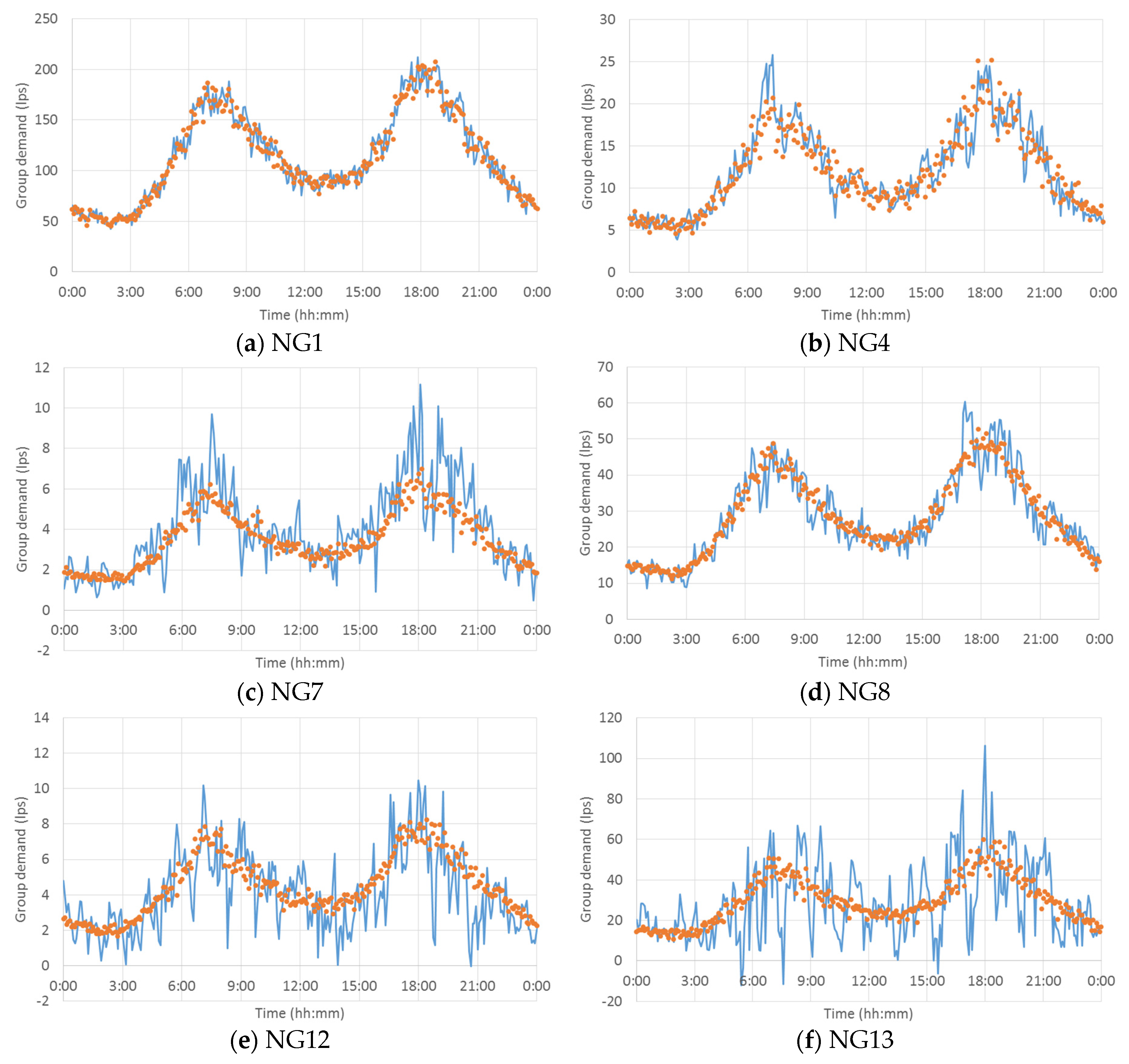
RMSE (L/s)	4.3	1.9	3.8	4.2	1.6	15.0	1.0

summarizes the RMSE of the individual node group demand estimates. Figure 10 plots the actual and estimated demands of representative multiple node groups (i.e., NG1, 4, 7, 8, 12 and 13). The non-linear KF was used as the unbiased minimum-variance estimator to minimize the error between two values. While accurate demand estimation was achieved in most node groups, the highest RMSE was obtained in NG13 followed by NG1 (Table 1 and Figure 10a,f, respectively). The latter mainly originated from the fact that NG1 had the largest base demand among the node groups (see the range of the y-axis in Figure 10a compared to the other plots in Figure 10). The node group with the largest base demand should have the largest error value if the proportion of error to the base demand value was assumed to stay similar or the same. In contrast, the former was caused by the lack of available information/signals for the demand estimation.

The nodes in NG13 were located along the transmission pipes that delivered bulk flows to supply the north, northeast and southwest parts of the study network (Figure 6 and Figure 9). While only a meter located at the source pipe linked to Source 1 could measure NG13’s demand (with other demands), the proportion of the group demand was very small compared to the total pipe flow (i.e., the total system demand because Source 2 was not operated) measured at the meter. NG13’s demand was less than the natural randomness of the total system demand (its base value was 726 L/s), which made it difficult to extract useful information from the measurements. This result led to the fluctuating demand with large deviation from the actual demand value (Figure 10f).

Similarly, fluctuating demand estimates with large deviations from the actual values were observed in node groups with a small base demand (e.g., NG7 and 12 in Figure 10c and e, respectively). In other words, the proportion of error seemed higher in these groups than the others. This result implied that the demand estimation was not reliable and difficult to utilize for management purposes. Such cases were avoided by placing meters at transmission pipes and distributing them among small pipes to capture the pipe flow information of various magnitudes, which was required for WDS demand estimation. The examples included a conventional meter located at the end of a branched network (delivering demand to one or two pendant nodes) or an AMI installed at the inlet pipe to each household.

5. Summary and Conclusions

State estimation is defined as the process of calculating a state variable of interest that is not directly measured. In a WDS, nodal demands are considered as the state variable (i.e., an unknown variable that cannot be directly measured) and can be estimated using nodal pressures and pipe flow rates measured at sensors installed throughout the system. The number of unknown variables should be minimized given the lack of available information for demand estimation. An alternative way is to group a set of nodes with a correlation (e.g., the same demand pattern and proximity). Finding the optimal node grouping that results in the best demand estimation accuracy is a challenging task given the number and location of meters and complex hydraulic conditions.

This study proposes an ONG model that minimizes the sum of the RMSEs of the node groups’ estimated demand given the number of node groups. The KF-based demand estimation method is linked with a genetic algorithm for node group optimization. The proposed model is applied to estimate the modified Austin network demand as a demonstration. The true demands and field measurements are synthetically generated using a hydraulic model of the study network. Note that the proposed model is the first to combine a WDS demand estimation tool (i.e., the KF-based model) and a node clustering/aggregation optimization model (i.e., eGA).

The sum of the RMSEs of the final best solution found with the proposed model is 56.2 L/s, which is about 76% of the value obtained by Jung and Lansey [8] based on their engineering judgment. In contrast to the randomly-generated initial solutions, the nodes are spatially grouped in the final solution. However, no apparent one-to-one linkage (mapping) is observed between a meter and a node group. This result indicates that the proposed ONG model should be applied to identify the best node grouping for the demand estimation of the loop-dominated networks. Among individual node groups, a high RMSE is obtained for the node group with the largest base demand. In addition, the proportion of the error to the true demand is large for node groups with a small base demand. Therefore, micrometers (i.e., meters that can measure a small flow, such as a conventional meter installed at pipes to dead-end nodes or AMIs) should be installed to further increase the demand estimation accuracy.

The work in this study has several limitations that future research must address. First, this model finds the optimal node grouping given that the number of node groups is predefined as equal to the number of meters. The model can be extended to include the number of node groups as a decision variable. Assuming that the same number of meters should be installed for an accurate demand estimation, the demand estimation problem can be formulated as a multi-objective problem that minimizes the sum of RMSEs and minimizes the cost of meters (i.e., meter instrument and installation costs). Many meters should be installed to achieve high demand estimation accuracy, which requires a large investment. Such a tradeoff relationship can be explored by solving the multi-objective demand estimation and meter placement problem.

Second, the proposed model can be verified using real demand data measured in a real large network fully equipped with AMI/automatic water meter reading.

Third, an advanced warm-start approach to the initial solution should be developed to shorten the time of finding a feasible solution in the early optimization phase. The Euclidean distance among nodes can be considered for the initial node grouping to avoid spatially-distributed nodes in a group. This study uses a loop-dominated network to demonstrate the proposed model. Different network types (e.g., branched or DMA-structured) can be used to check (1) whether the conclusions of this study are still valid or not and (2) whether such network layouts affect the demand estimation accuracy and optimal node grouping or not. Finally, the proposed model can serve as a submodule for WDS operation and management tools (e.g., a real-time WDS operation model that determines the status of pumping units given the estimated future demand).