Development of a Watershed-Scale Long-Term Hydrologic Impact Assessment Model with the Asymptotic Curve Number Regression Equation

Abstract

In this study, 52 asymptotic Curve Number (CN) regression equations were developed for combinations of representative land covers and hydrologic soil groups. In addition, to overcome the limitations of the original Long-term Hydrologic Impact Assessment (L-THIA) model when it is applied to larger watersheds, a watershed-scale L-THIA Asymptotic CN (ACN) regression equation model (watershed-scale L-THIA ACN model) was developed by integrating the asymptotic CN regressions and various modules for direct runoff/baseflow/channel routing. The watershed-scale L-THIA ACN model was applied to four watersheds in South Korea to evaluate the accuracy of its streamflow prediction. The coefficient of determination (R²) and Nash–Sutcliffe Efficiency (NSE) values for observed versus simulated streamflows over intervals of eight days were greater than 0.6 for all four of the watersheds. The watershed-scale L-THIA ACN model, including the asymptotic CN regression equation method, can simulate long-term streamflow sufficiently well with the ten parameters that have been added for the characterization of streamflow.

1. Introduction

In recent years, environmental disasters, such as droughts and floods, caused by climate changes have increased in occurrence, and various approaches to finding solutions for these issues have been suggested and investigated [1,2,3,4]. Estimation of runoff in watersheds is very important to preventing droughts and floods, preserving the ecological integrity of aquatic systems and managing water quality [5,6,7]. There are two ways to estimate the runoff in a watershed: monitoring of streamflow and use of rainfall–runoff models.

Monitoring of streamflow is more accurate than the use of computer models in estimating runoff in a watershed. However, it can be difficult to measure streamflow in all of the subbasins in a watershed without appropriate manpower and financial resources. In addition, it can be difficult to collect streamflow data during flooding and typhoon seasons [8]. Furthermore, for sustainable watershed management, prediction of future streamflow changes with climate/land use changes should be considered. For these reasons, watershed-scale continuous rainfall–runoff models have been widely used for management of hydrology and environment plans because these computer models can be used to estimate the long-term streamflow at gauged/ungauged subbasins efficiently [9,10,11,12,13].

There are many computer rainfall–runoff models available for use in estimating runoff, including SWAT (Soil and Water Assessment Tool) [14], L-THIA (Long-Term Hydrologic Impact Assessment) [15,16,17], SWMM (Storm Water Management Tool) [18,19] and STEPL (Spreadsheet Tool for Estimating Pollutant Load) [20,21], among others. Most of these models calculate direct runoff using the Curve Number (CN) method proposed by the Natural Resources Conservation Service (NRCS-CN) [22].

The L-THIA model is simpler than some other models, such as SWAT and HSPF. In addition, the L-THIA model can calculate direct runoff and pollutant loads with a limited number of input parameters, such as rainfall data, land cover and hydrologic soil group data [15,17]. The L-THIA model has been developed in web and ArcGIS versions [23,24,25,26,27]. It has been used in the calculation of runoff and pollutant loads in many studies. Recently, a version of the L-THIA model with low-impact development (LID) capability was developed and has been used for efficient watershed management purposes, such as the determination of Total Maximum Daily Loads (TMDLs), in the USA [28].

However, the NRCS-CN method used in the L-THIA model cannot be used to calculate direct runoff accurately during low-flow seasons because the static CN value considered in the NRCS-CN method does not explain the relationship between rainfall and asymptotic CN, especially for lower-rainfall–CN datasets [29].

According to the relationships between rainfall and CN suggested by numerous rainfall–runoff datasets [30], the CN decreases as the rainfall increases and converges to an asymptotic CN. However, some previous studies on the asymptotic CN method [30,31,32,33,34,35,36] have been limited in that they have considered only ungaged watersheds, whereas other studies have considered only gaged watersheds and have employed regression equations from datasets for gaged watersheds in direct runoff estimation.

To overcome this limitation, thirteen Land Cover-based Asymptotic CN (ACN) Regression Equations (LC-ACN-REs) were proposed for the estimation of runoff in ungaged watersheds, and these equations were applied to TMDL watersheds in South Korea [29]. The results of comparisons between observed and estimated runoff indicated that LC-ACN-REs can simulate direct runoff very well in comparison to the NRCS-CN method. Although LC-ACN-REs have been proven to be efficient tools for accurate estimation of direct runoff, they are still limited in that the effects of hydrologic soil groups on direct runoff estimation cannot be simulated.

The L-THIA model has been used for runoff estimation on the watershed scale [16,25,26,37]. However, the L-THIA model is not applicable to larger watersheds, because it does not consider the lag time for direct runoff to reach streams, which could be more than one day, meaning that only a fraction of the direct runoff will flow into streams on the day of simulation [38]. In addition, the current L-THIA model does not simulate baseflow and channel routing within watershed structures and does not consider point source discharge.

The objectives of this study were as follows: (1) to extend the available LC-ACN-REs to consider hydrologic soil groups (A,B,C,D), as described in the NEH-4 CN (National Engineering Handbook Chapter 4) table [22]; (2) to develop a watershed-scale model of the Long-term Hydrologic Impact Assessment with the extended LC-ACN-REs (the watershed-scale L-THIA ACN model) by adding modules for direct runoff, baseflow and channel routing; and (3) to evaluate this LC-ACN-RE-enhanced watershed-scale L-THIA ACN model with soil component, lag time, baseflow and channel routing capabilities.

2. Materials and Methods

2.1. LC-ACN-RE Approach to Considering Hydrologic Soil Groups

In the project “Long-term monitoring of Nonpoint Source (NPS) pollution” funded by the Ministry of Environment (MOE) of South Korea, runoff and water quality samples were collected for each representative land cover type rather than for specific Hydrologic Soil Groups (HSGs) or other soil infiltration properties. Thus, the LC-ACN-REs developed by [29] were classified as being applicable by land cover type; the effects of soil infiltration properties on direct runoff estimation cannot be analyzed with LC-ANC-RE approaches.

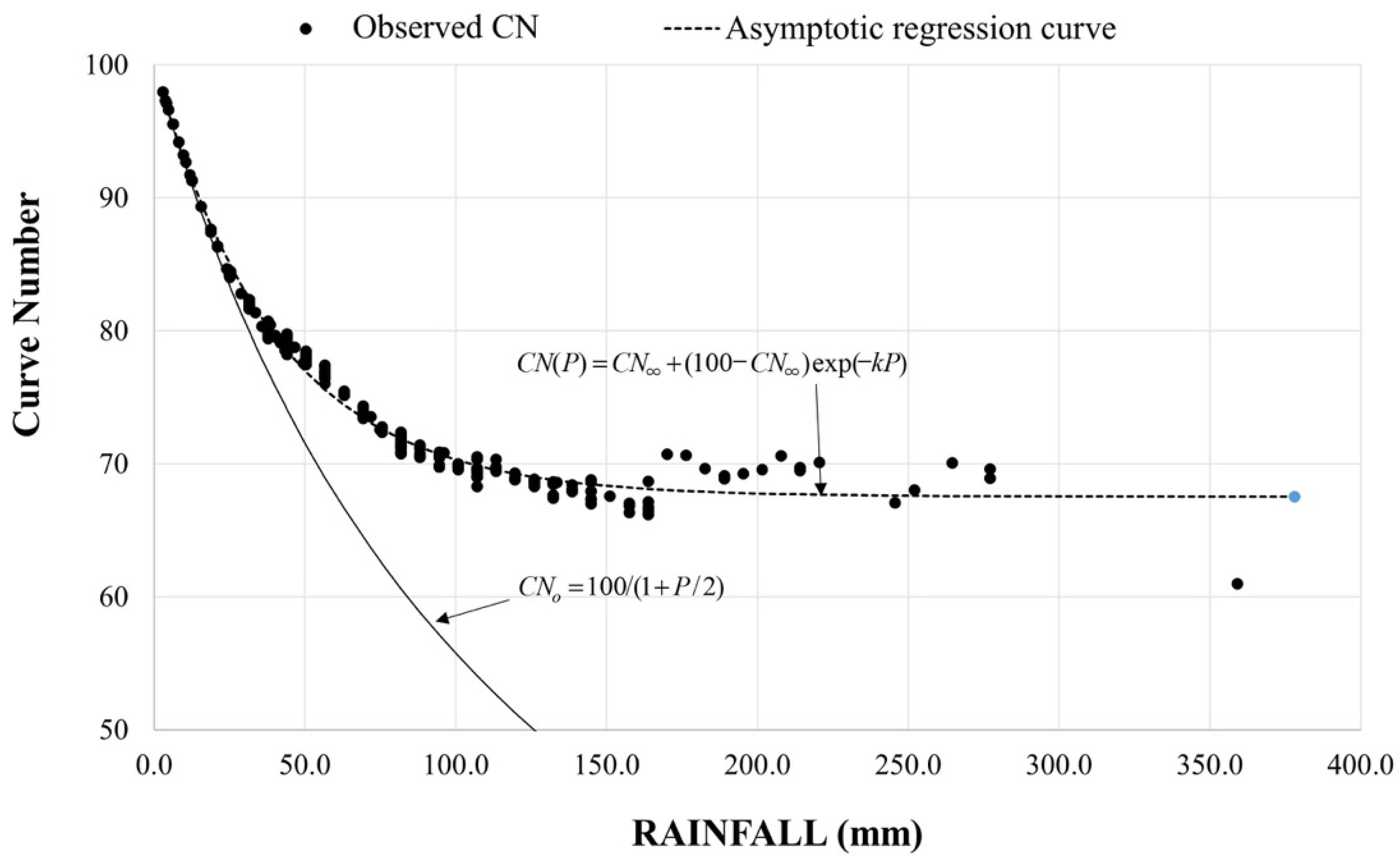
To overcome this limitation of the LC-CAN-REs [29], rainfall and direct runoff data from the “Long-term monitoring of Nonpoint-Source (NPS) pollution” project were analyzed to obtain the CN value for each combination of rainfall and direct runoff using Equation (1), which was proposed by Hawkins [30]. HSG information for the monitoring site was then compiled for use in estimating CN values for other HSGs. The CN values for other HSGs were estimated by multiplying the CN values obtained using Equation (1) by the ratios of the CN values for other HSGs in the NEH-4 CN table (

Table 1. CN values for thirteen land cover types and Hydrologic Soil Groups (HSGs) from Land Cover-based Asymptotic CN Regression Equations (LC-ACN-REs). NEH-4, National Engineering Handbook Chapter 4.

Name of the Land Cover in LC-ACN-RE Approach	CN Value in NEH-4 CN Table for Individual Soil Type [22]
	A	B	C	D
Residential area	77	85	90	92
Manufacturing area	81	88	91	93
Regional public facility area	89	92	94	95
Recreational facility area	89	92	94	95
Road	98	98	98	98
Commercial area	89	92	94	95
Upland	62	71	78	81
Orchard	62	71	78	81
Greenhouse	62	71	78	81
Paddy	62	71	78	81
Pasture	30	58	71	78
Forest	45	66	77	83
Bare land	77	86	91	94

). After obtaining the CN values for 13 land cover types and four HSG combinations, 52 asymptotic regression equations, such as the following, were obtained from regression analysis, as illustrated in Figure 1 (Equation (2) [30]).

$$CN=25400/254+5[P+2Q-\sqrt{4Q^2+5PQ}]$$

(1)

where Q is the direct runoff (mm) and P is the rainfall (mm).

$$CN(P)=C{N}_{\infty }+(100-C{N}_{\infty })\exp (-kP)$$

(2)

where CN_∞ is the asymptotic CN value, P is the rainfall (mm) and k is a fitting constant.

2.2. Development of the Watershed-Scale L-THIA ACN Model

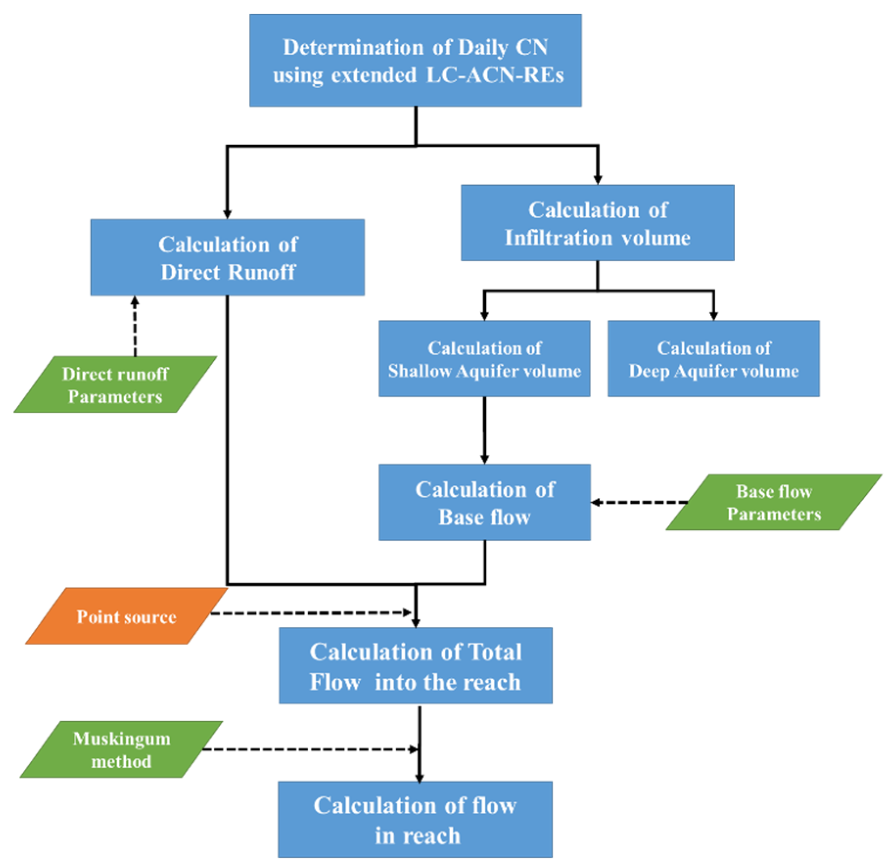
The watershed-scale L-THIA ACN model developed in this study consists of three modules, for direct runoff, baseflow (with extended LC-ACN-REs developed as described in Section 2.1) and channel routing capabilities (Figure 2). The model requires daily rainfall, point source data and hydrological response unit (HRU) mapping created by combining a subbasin map, a soil map and a land use map.

2.2.1. Development of the Direct Runoff Estimation Module

As explained above, the 52 asymptotic regression equations (Equation (2)) were obtained for 13 land cover types and four HSGs. Using these equations, the CN values for a given set of daily rainfall data were computed for all land cover and HSG combinations for each watershed studied.

According to various studies on the NRCS-CN method, CN values can be adjusted based on the slope in a watershed [39], as well as for various local conditions that affect rainfall–runoff. Thus, an adjustment coefficient was added to explain the effect of the slope on the CN values (Equation (3)). In this study, the limits of the range for the adjustment coefficient for CN were set to −0.1 and +0.1 (−10% and +10%).

$$Adj\_C{N}_{HRU}=C{N}_{HRU,ACN}\times Adj\_CN$$

(3)

where CN_HRU is the adjusted CN value for HRU, Adj_CN_{HRU, ACN} is the CN value determined from the extended LC-ACN-REs and Adj_CN is the adjusted coefficient for CN.

After adjustment of the CN values, the direct runoff of each HRU was estimated (Equation (4)).

$${Q^1}_{DR,HRU}=\frac{{(P-0.2S)}^2}{(P+0.8S)},P\ge 0.2S,S=\frac{25400}{Adj\_C{N}_{HRU}}-254$$

(4)

where Q¹_DR,HRU is the amount of direct runoff generated by an HRU for each day (mm), P is the rainfall (mm), S is the potential maximum retention (mm) and Adj_CN_HRU,ACN is the adjusted coefficient for CN.

In a large-scale watershed, the amount of direct runoff that occurs on a day can be lagged, and only a portion of the direct runoff will flow into a stream on a day. Thus, in this study, the direct runoff delay process was addressed in the module in the form of an exponential function of the time of concentration (TC) and the lag coefficient (DR_lag), as proposed in the SWAT model (Equation (5)) [38].

Once the direct runoff of each HRU is calculated using Equation (4), the amount of direct runoff flowing into the stream can be calculated using Equation (5).

$$Q_{DR,HRU}=({Q^1}_{DR,HRU}+Q_{stor,i-1})\times \left(1-\exp \left[\frac{-D{R}_{lag}}{TC}\right]\right)$$

(5)

where Q_DR,HRU is the amount of direct runoff discharged to the main channel on a given day (mm), Q¹_DR,HRU is amount of direct runoff generated by the HRU on a given day (mm), Q_stor is the direct runoff lagged from the previous day, DR_lag is the direct runoff lag coefficient and TC is the time of concentration (h).

The value of the lag coefficient (DR_lag) ranges from 1 to 12 and should be provided by the user after investigating watershed characteristics or related documents. The time of concentration is defined as the time required for water to flow from a remote point in a watershed to a watershed outlet. The time of concentration is important in the rainfall runoff model and can be estimated from various formulas, although the variability of the estimates of the time of concentration given by various formulas can be high [40]. There are two types of time of concentration: the time required for overland flow and the time required for channel flow. These are calculated from watershed-specific information, such as the average slope (m/m), the slope length (m), the channel length from the most distant point to the subbasin outlet (km) and Manning′s coefficient, n, as shown in Equations (6) and (7) [38,41]. Equations (4) and (5) were added to the direct runoff module of the watershed-scale L-THIA ACN model.

$$T{C}_o=\frac{{L_{slope}}^{0.6}\cdot n^{0.6}}{18\cdot Slop{e}^{0.3}}$$

(6)

$$T{C}_c=\frac{0.62\cdot L\cdot {n_c}^{0.75}}{Are{a}^{0.125}\cdot Slop{e_c}^{0.375}}$$

(7)

In these equations, TC_O is the time of concentration for overland flow (h); TC_C is the time of concentration for channel flow (h); L_Slope is the HRU slope length (m); n is Manning′s coefficient for overland flow; n_C is Manning’s coefficient for channel flow; Slope is the average slope of the HRU (m/m); Slope_C is the channel slope (m/m); L is the channel length from the most distant point to the subbasin outlet (km); and Area is the area of the HRU (km²).

In this study, the values of Manning’s coefficient from

Table 2. Manning’s roughness coefficient, n, for overland flow [42].

Land Cover	Median	Range
Fallow, no residue	0.010	0.008–0.012
Conventional tillage, no residue	0.090	0.060–0.120
Conventional tillage, residue	0.190	0.16–0.220
Chisel plow, no residue	0.090	0.060–0.120
Chisel plow, residue	0.130	0.100–0.160
Fall disking, residue	0.400	0.300–0.500
No till, no residue	0.070	0.040–0.100
No till, 0.5–1 t/ha residue	0.120	0.070–0.170
No till, 2–9 t/ha residue	0.300	0.170–0.470
Rangeland, 20% cover	0.600	–
Short-grass prairie	0.150	0.100–0.200
Dense grass	0.240	0.170–0.300
Bermuda grass	0.410	0.300–0.480

were used for the calculation of TC_O, and the values of Manning’s coefficient for TC_C were calibrated based on the land cover and the parameter range, based on Table 2. The Slope, the Area of the HRU and the channel length L from the most distant point to the subbasin outlet (km) were calculated using a GIS tool for the purpose of computing the time of concentration for overland flow and the time of concentration for channel flow.

However, because the calculation of the slope length is strongly affected by the digital elevation model (DEM) cell size, the field slope length can be overestimated when it is calculated using a GIS tool [43]. Furthermore, the DEM resolution, slope length, river networks and flow length estimation are among the major source of uncertainties in rainfall–runoff modeling [44]. Thus, in this study, the slope length of each HRU was calculated from the relationship between the field slope length and the average field slope, as proposed in [45]. This relationship between the field slope length and the average field slope (

Table 3. Suggested maximum slope length for field slope for contouring [45].

Land Slope (%)	Maximum Length (m)
1–2	122
3–5	91
6–8	61
9–12	37
13–16	24
17–20	18
21–25	15

) was added to the direct runoff module in the watershed-scale L-THA ACN model. However, this relationship, described in Table 3, was obtained from measurements made in the USA. Thus, to reflect local field slope length properties, an additional parameter (SLSUB) was added to adjust the slope length.

After calculation of the direct runoff for each HRU released to the stream, the direct runoff of each subbasin was calculated by summing the direct runoff from all HRUs within each subbasin (Equation (8)):

$$Q_{DR,sub}={\displaystyle \sum _{HRU=1}^n{Q}_{DR,HRU}}$$

(8)

where Q_DR,sub is the amount of direct runoff generated in the subbasin on a given day (mm).

2.2.2. Development of Baseflow Module

The NRCS-CN method and LC-ACN-REs are both used for direct runoff estimation, but not for baseflow computation for a watershed. The baseflow component was developed and linked to the watershed-scale L-THIA ACN model for use in watershed hydrology studies, as well as evaluation of the water quality of a watershed.

According to Dingman [46], the aquifer in a watershed is composed of two aquifers, an unconfined aquifer and a confined aquifer. Water recharged into an unconfined aquifer contributes to flow in the main channel and influences the amount of streamflow, while water recharge into a confined aquifer is assumed to flow somewhere outside of the watershed [47].

Based on the user-defined fraction of infiltrated water flowing into the confined aquifer from each HRU, the amount of infiltrated water flowing into the unconfined aquifer can be estimated. The baseflow module, which was developed and integrated into the watershed-scale L-THIA ACN model, simulates these processes to account for the baseflow contribution to streamflow in a watershed. The water balance in an unconfined aquifer is calculated according to Equation (9):

$$aq{f}_{HRU,i}=aq{f}_{HRU,i-1}+{\omega }_{unconf,HRU}-Q_{BF,HRU}$$

(9)

where aqf_HRU,i is the amount of water stored in an unconfined aquifer on a given day (mm), aqf_HRU,i-1 is the amount of water stored in the unconfined aquifer on the previous day (mm), ω_unconf,HRU is the amount of recharge entering the unconfined aquifer on that day (mm) and Q_BF,HRU is the amount of baseflow into the main channel (mm).

The amount of water recharged into both aquifers (confined and unconfined) is estimated using the exponential decay weighting function (Equation (10)) proposed by Venetis [48] and used by Sangrey et al. [49] in their precipitation–groundwater response model and by Neitsch et al. [38] in the SWAT model:

$${\omega }_{rchrg,HRU,i}=\left[1-\exp \left(\frac{-1}{B{F}_{delay}}\right)\right]\times F_{HRU,i}+\exp \left(\frac{-1}{B{F}_{delay}}\right)\times {\omega }_{rchrg,HRU,i-1}$$

(10)

where ω_rcharg,HRU,i is the amount of recharge entering both aquifers on a given day (mm), BF_delay is the delay time in aquifer recharge once the water infiltrates from the surface (days), F_HRU,i is the amount of infiltration on the given day (mm) and ω_{rcharg,,HRU,i-1} is the amount of recharge that enters the aquifers on the previous day (mm).

The amount of infiltration on a given day is calculated using Equation (11), which is modified from that used in the NRCS-CN method [22] and was used by Kim et al. [50] to estimate the CN-based infiltration and baseflow:

$$F_{hru,i}=\frac{S(P-I_a)}{P-I_a+S},I_a=0.2S,S=\frac{25400}{Adj\_C{N}_{HRU,ACN}}-254$$

(11)

where F_HRU,i is the amount of infiltration on a given day (mm), S is the is the potential maximum retention (mm), P is the rainfall (mm), Adj_CN_HRU, _ACN is the CN value determined from the extended LC-ACN-REs and I_a is the initial abstraction (mm).

In the baseflow module, only a fraction of the infiltrated water is assumed to flow into the unconfined aquifer, based on the user-defined fraction of infiltrated water flowing into the confined aquifer (Equations (12) and (13)):

$${\omega }_{conf,HRU}=F{r}_{conf}\times {\omega }_{rchrg,HRU}$$

(12)

$${\omega }_{unconf,HRU}={\omega }_{rchrg,HRU}-{\omega }_{conf,HRU}$$

(13)

where ω_conf,HRU is the amount of infiltrated water flowing into a confined aquifer on a given day (mm), Fr_conf is the fraction of water flowing into the confined aquifer and ω_unconf,HRU is the amount of recharge entering the unconfined aquifer on that day (mm).

The amount of water flowing into an unconfined aquifer contributes to baseflow only if the amount of water in the unconfined aquifer exceeds a threshold value specified by the user that depends on the aquifer′s characteristics. The steady-state response of the baseflow is expressed by Equation (14) [51]:

$$Q_{BF,HRU}=\frac{8000\times k_{sat}}{{L^2}_{BF}}\times h_{wtbl}$$

(14)

where Q_BF,HRU is the amount of baseflow into the main channel (mm), k_sat is the hydraulic conductivity of the aquifer (mm/day), L_BF is the distance from the ridge or subbasin divide for the baseflow to the main channel (m) and h_wtbl is the water table height (m).

The water table height (h_wtbl) depends on the baseflow response in the non-steady state and is calculated using Equation (15) [52]:

$$\frac{d{h}_{wtbl}}{dt}=\frac{{\omega }_{unconf,HRU}-Q_{BF,HRU}}{800\times \mu }$$

(15)

where $\frac{d{h}_{wtbl}}{dt}$ is the change in the elevation of the water table (mm/day), ${\omega }_{unconf,HRU}$ is the amount of recharge entering the unconfined aquifer on a given day (mm), Q_BF,HRU is the baseflow into the main channel on that day (mm) and μ is the specific yield of the unconfined aquifer (m/m).

Combining Equations (14) and (15) yield Equation (16) [38]:

$$\frac{d{Q}_{BF,HRU}}{dt}=10\times \frac{k_{sat}}{\pi \times {L^2}_{BF}}\times ({\omega }_{unconf,HRU}-Q_{BF,HRU})={\alpha }_{BF}\times ({\omega }_{unconf,HRU}-Q_{BF,HRU})$$

(16)

where Q_BF,HRU is the baseflow into the main channel on a given day (mm), k_sat is the hydraulic conductivity of the aquifer (mm/day), L_BF is the distance from the ridge or subbasin divide for the baseflow to the main channel (m), μ is the specific yield of the unconfined aquifer (m/m), ω_unconf,HRU is the amount of recharge entering the unconfined aquifer on that day (mm) and α_BF is the baseflow recession constant.

After integrating and rearranging Equation (14), Q_BF, _HRU can be expressed by Equation (17) [38]:

$$\begin{array}{l}{Q}_{BF,HRU,i}=Q_{BF,HRU,i-1}\times \exp [-{\alpha }_{BF}\times \Delta t]+{\omega }_{unconf,HRU}\times (1-\exp [-{\alpha }_{BF}\times \Delta t]),if aqf>aq{f}_{thr}\\ Q_{BF,HRU,i}=0,if aqf<aq{f}_{thr}\end{array}$$

(17)

where Q_BF,HRU,i is the baseflow into the main channel on a given day (mm), Q_BF,HRU,i-1 is the baseflow into the main channel on the previous day, α_BF is the baseflow recession constant, ω_unconf,HRU is the amount of recharge entering the unconfined aquifer on the given day (mm), ∆t is the time step (one day), aqf is the amount of water stored in the unconfined aquifer on the given day (mm) and aqf_thr is the threshold water level in the unconfined aquifer for baseflow contribution to the main channel to occur (mm).

The baseflow recession constant (α_BF) in Equation (17) reflects the baseflow response to the amount of recharge [52]. Values between 0.1 and 0.3 represent slow response conditions in a watershed, and values between 0.9 and 1.0 represent rapid response conditions [38,52]. Two options (simple long-term daily average and daily time series point source capabilities) were enabled in the direct runoff module to simulate the effects of discharge from Waste Water Plants (WWP) or other point sources on watershed hydrology and water quality.

2.2.3. Development of Channel Routing Module

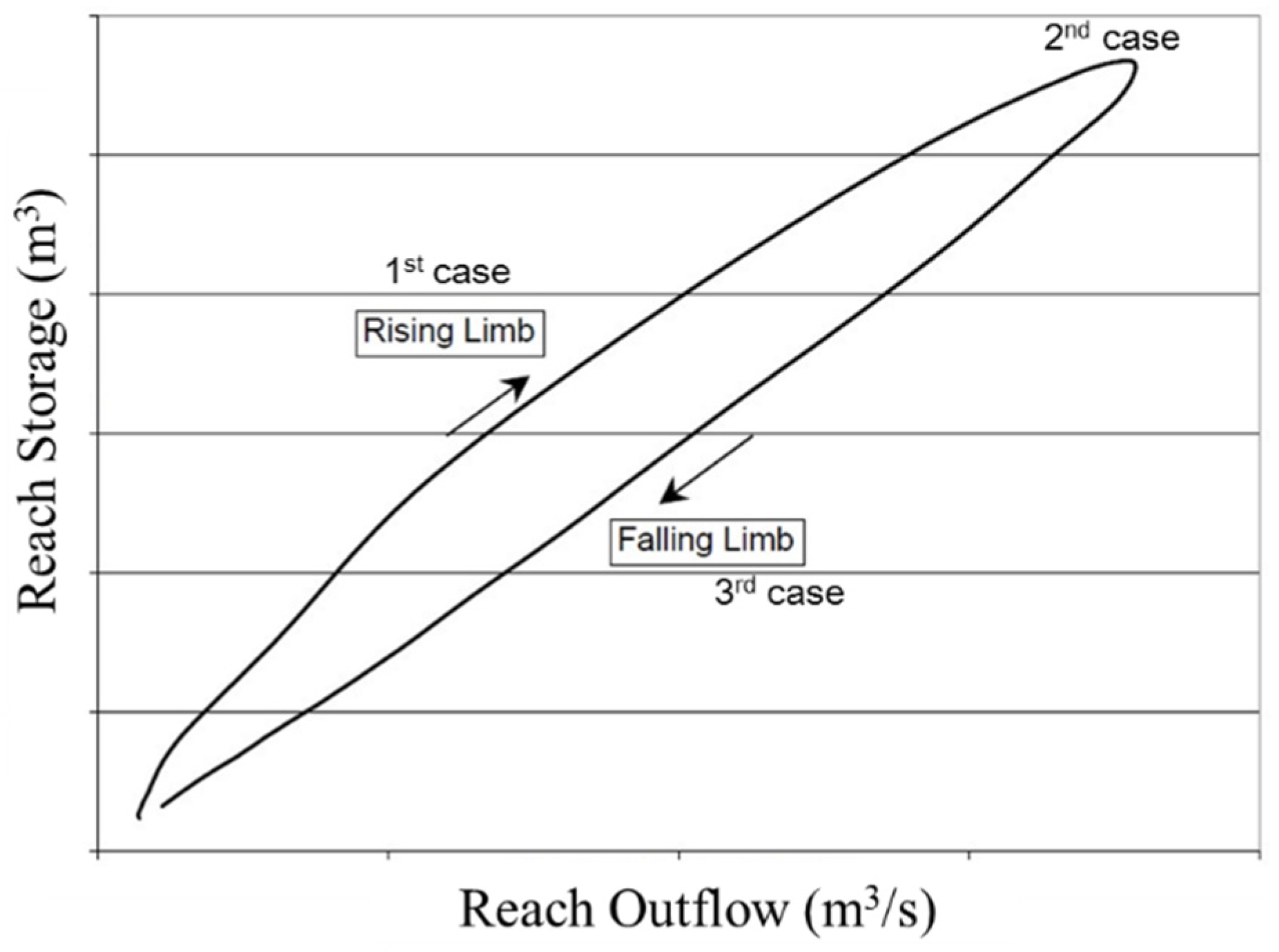
Streamflow flows downward and meets flow from other upper streams in channel networks. The amount of streamflow in a watershed is affected by various mechanisms. In this study, a channel routing module was integrated into the watershed-scale L-THIA ACN model for simulation of flow routing using the Muskingum routing method [53]. The Muskingum routing method estimates the storage volume in a channel length as a combination of wedge and prism storage [53]. The concept of the Muskingum routing method is illustrated in Figure 3. The first case represents the storage in the river during the rising limb of a hydrograph; the second case represents uniform flow; and the third case represents the storage during the falling limb of the hydrograph. This hysteresis might cause different flood wave speeds during the rising and falling limbs of the hydrograph [54].

The effects of these variables and the reach storage–discharge relationship are expressed by the equation used in the Muskingum routing method to estimate the reach storage volume, V_stor:

$$V_{stor}=K(X{q}_{in}+(1-X)q_{out})$$

(18)

where V_stor is the reach storage volume (m³/s), K is the storage time constant for the reach (s), X is the weighting factor, q_in is the inflow rate (m³/s) and q_out is the outflow rate (m³/s).

Equations (18) and (19), proposed by Williams [55], can be combined and simplified as Equation (20):

$$\Delta t\left(\frac{q_{in}+q_{in,\Delta t}}{2}\right)-\Delta t\left(\frac{q_{out}+q_{out,\Delta t}}{2}\right)+V_{stor}=V_{stor,\Delta t}$$

(19)

$$q_{out,\Delta t}=C_1{q}_{in,\Delta t}+C_2{q}_{in}+C_3{q}_{out}$$

(20)

where q_in is the inflow rate at the beginning of the time step (m³/s), q_in,∆t is the inflow rate at the end of the time step (m³/s), q_out is the outflow rate at the beginning of the time step (m³/s), q_out,∆t is the outflow rate at the end of the time step (m³/s) and C1, C2 and C3 are expressed by Equations (21)–(23), respectively.

$$C_1=\frac{\Delta t-2\times K\times X}{2\times K\times (1-X)+\Delta t}$$

(21)

$$C_2=\frac{\Delta t+2\times K\times X}{2\times K\times (1-X)+\Delta t}$$

(22)

$$C_3=\frac{2\times K\times (1-X)-\Delta t}{2\times K\times (1-X)+\Delta t}$$

(23)

The value for the weighting factor, X, is a user input. The value of the storage time constant, K, is calculated using Equation (24):

$$K=Mk1\times bankfull+Mk2\times bankful{l}_{0.1}$$

(24)

where K is the storage time constant for a reach segment (s), Mk1 and Mk2 are weighting factors input by the user, bankfull is the storage time constant estimated for the reach segment with bankfull flows (s) and bankfull_0.1 is the storage time constant estimated for the reach segment with one tenth of the bankfull depth (s).

The value of bankfull can be calculated using Equation (25) [38,53]:

$$bankfull=\frac{1000\times L_{reach}}{c}$$

(25)

where bankfull is the storage time constant estimated for the reach segment with bankfull flows (s), L_reach is the stream length (m) and c is the celerity corresponding to the flow for the specified depth (m/s).

The value of c can be determined from Equation (26), using the cross-sectional area of the stream and Manning’s equation [38]:

$$c=\frac{d}{dA}(q_{ch})=\frac{5}{3}\left(\frac{R^{\frac{2}{3}}\times I^{\frac{1}{2}}}{n}\right)=\frac{3}{5}\cdot v_c$$

(26)

where A is the cross-sectional area of flow in the stream (m²), q_ch is the flow rate in the stream (m³/s), R is the hydraulic radius for a given depth of flow (m), I is the slope (m/m) and n is Manning’s coefficient for the channel.

To calculate V_c in Equation (26), the metacenter of the streams should be evaluated, and the actual shapes of all of the streams in each subbasin should be measured. However, it would be difficult to measure the cross-sections of all of the streams. In this study, all streams in subbasins were assumed to be trapezoidal channels with side slopes of 0.5, and the slope of the flood plain was assumed to be 0.25. These assumptions are similar to those made in the SWAT model [38].

2.3. Input Parameters of Watershed-Scale L-THIA ACN Model

The watershed-scale L-THIA ACN model was developed to estimate streamflow using direct runoff, baseflow and channel routing modules.

The parameters of these three modules consist of CN parameters for all HRUs, two direct runoff parameters, four baseflow parameters and three channel routing parameters, as summarized in

Table 4. Parameters used in the watershed-scale L-THIA ACN model.

Calibration Component	Calibration Parameter	Description of Parameter	Range of Parameter
Direct runoff	Adj_CN (1)	Adjusted coefficient for CN	−0.1–0.1
	DRlag (1)	Direct runoff lag coefficient	1–12
	SLSUB (2)	Adjustment for slope length	−10–10
Baseflow	αBF (1)	Baseflow recession constant	0.1–1.0
	Frconf (1)	Fraction of water flowing into confined aquifer	0.0–0.9
	aqfthr (1)	Threshold water level in the unconfined aquifer for baseflow contribution (mm)	0.0–5000
	BFdelay (1)	Delay time for aquifer recharge after water infiltration from surface (day)	1–10
Channel routing	MK1 (1)	Weighting factor for influence of normal flow on storage time constant value	0.1–0.9
	Mk2 (1)	Weighting factor for influence of low flow on storage time constant value	0.1–0.9
	Mkx (1)	Weighting factor for Muskingum method	0.1–0.9

Note: (1) constant value; (2) multiplied value.

. The watershed-scale L-THIA ACN model requires a smaller number of parameters than other watershed models, such as SWAT and HSPF.

2.4. Applications of Watershed-Scale L-THIA ACN Model

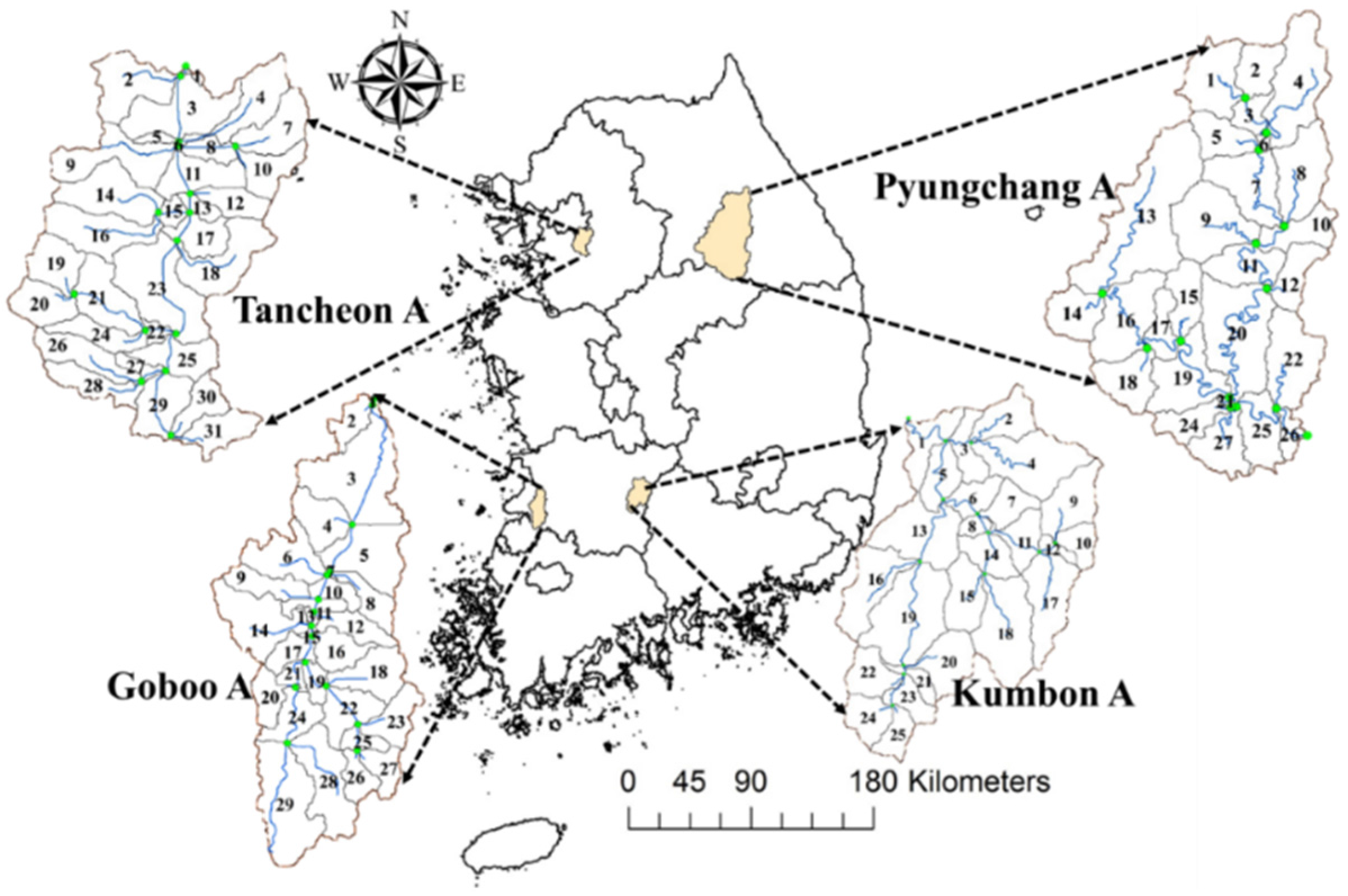
The watershed-scale L-THIA ACN model, developed in this study, was applied to four watersheds (Goboo A, Tancheon A, Kumbon A and Pyungchang A) in South Korea, where TMDLs have been implemented to evaluate the water quality achieved with various management practices (Figure 4).

Among the four watersheds, the Goboo A watershed (231.9 km²) has a somewhat flatter topography, with average slopes (5.0%). The land cover distribution is forest (13.6%), urban (5.7%), agricultural (71.6%), pasture (3.7%), bare land (0.9%) and other (4.6%). The areas of the Tancheon A, Kumbon A and Pyungchang A watersheds are 203.9, 289.3 and 1756.9 km², respectively, and the average slopes of these three watersheds are 14.6, 25.7 and 30.8%, respectively.

The land cover distributions of the Tancheon A, Kumbon A and Pyungchang A watersheds are forest (50.3, 65.9 and 80.5%, respectively), urban (25.3, 2.7 and 1.7%, respectively), agricultural (5.3, 20.8 and 12.8%, respectively), pasture (13.8, 7.7 and 2.0%, respectively), bare land (3.9, 1.4 and 1.2%, respectively) and other (1.3, 1.6 and 1.9, respectively). The Goboo A, Tancheon A and Kumbon A watersheds are headwater watersheds. The Pyungchang A watershed is considerably larger than these other three watersheds and includes the Jucheon A headwater watershed.

The watershed-scale L-THIA ACN model requires daily rainfall data, as well as HRU maps, which are prepared from combinations of subbasin, land cover and soil maps. Subbasin maps were delineated by 30-m resolution DEM and stream data using the ArcGIS watershed delineation geoprocessing tool. HRU maps were created by combining subbasin maps, reconnaissance soil maps and land cover maps provided by the Ministry of Environment of South Korea.

Daily streamflows for 1 January 2010–31 December 2014 were estimated for the four watersheds using the watershed-scale L-THIA ACN model and precipitation data from the Korean Meteorological Administration (KMA). The watershed-scale L-THIA ACN model was calibrated and validated by adjusting the parameters of the direct runoff and baseflow to fit the simulated daily streamflows for eight-day intervals to observed streamflow data. The calibration period was 1 January 2008–31 December 2010 and the validation period was 1 January 2011–12 December 2014.

3. Results and Discussion

3.1. Result of Extended LC-ACN-RE Approach for the Consideration of HSGs

In this study, thirteen land cover-based asymptotic CN regression equations (LC-ACN-REs) were extended to 52 regression equations to consider HSGs, using the ratio of CN for a given HSG in the NEH-4 CN table (

Table 5. Parameters of extended LC-ACN-REs with HSG considered.

Land Cover	Soil Type	Asymptotic CN Regression
		$\mathit{C}{\mathit{N}}_{\mathbf{\infty }}$	$\mathbf{100}\mathbf{-}\mathit{C}{\mathit{N}}_{\mathbf{\infty }}$	K
Residential area	A	74.43	25.57	0.0417
	B	82.20	17.80	0.0124
	C	86.72	13.28	0.0059
	D	88.61	11.39	0.0048
Manufacturing area	A	60.69	39.31	0.0282
	B	67.69	32.31	0.0169
	C	70.69	29.31	0.0128
	D	72.70	27.30	0.0104
Commercial area	A	86.19	13.81	0.0593
	B	89.09	10.91	0.0376
	C	91.03	8.97	0.0263
	D	92.00	7.47	0.0185
Recreational facility area	A	80.29	19.71	0.0677
	B	83.00	17.00	0.0550
	C	84.80	15.20	0.0427
	D	85.70	14.30	0.0428
Road	A	66.27	33.73	0.0110
	B	66.27	33.73	0.0110
	C	66.27	33.73	0.0110
	D	66.27	33.73	0.0110
Paddy	A	55.34	44.66	0.0515
	B	63.37	36.63	0.0312
	C	69.62	30.38	0.0224
	D	72.30	27.70	0.0191
Upland	A	38.84	61.16	0.0144
	B	47.84	52.16	0.0077
	C	54.84	45.16	0.0044
	D	57.84	42.16	0.0033
Green house	A	41.34	58.66	0.0355
	B	47.35	52.65	0.0198
	C	52.13	47.87	0.0123
	D	54.13	45.87	0.0077
Orchard	A	48.77	51.23	0.0274
	B	55.84	44.16	0.0204
	C	61.35	38.65	0.0157
	D	63.71	36.29	0.0176
Forest	A	36.07	63.93	0.0362
	B	52.91	47.09	0.0274
	C	60.46	39.54	0.0141
	D	64.84	35.16	0.0117
Pasture	A	22.99	75.77	0.0181
	B	34.09	65.91	0.0164
	C	40.33	59.67	0.0164
	D	43.95	56.05	0.0164
Bare land	A	74.76	25.24	0.0200
	B	82.59	17.41	0.0092
	C	87.13	12.87	0.0072
	D	89.91	10.09	0.0066

). Thus, the CN values for each HSG group can be estimated with the 52 extended LC-ACN-REs. These CN values were used to estimate the direct runoff, the infiltration from each HRU and the baseflow component.

The 52 extended regression equations predict the lowest asymptotic CN values for high-permeability soils of the HSG A type and the highest asymptotic CN values for low-permeability soils of the HSG D type. The highest asymptotic CN value predicted by these equations was 92.0 for commercial areas, and the lowest asymptotic CN value was 23.0 for pasture.

3.2. Application of the Watershed-Scale L-THIA ACN Model

The watershed-scale L-THIA ACN model was calibrated using observed streamflow data for the four study watersheds in South Korea. The calibrated values of the ten parameters for each study watershed are shown in

Table 6. Calibrated and validated model parameters for streamflow simulation using the watershed-scale L-THIA ACN model.

Watershed	Adj_CN	SLSUB	DRlag	αBF	aqfthr	Frconf	BFdelay	Mk1	Mk2	Mkx
Goboo A	−0.04	7.0	3	0.5	5.0	0.05	1	0.05	0.95	0.2
Tancheon A	0.06	1.0	6	0.5	5.0	0.03	2	0.10	0.90	0.1
Kumbon A	0.07	1.0	7	0.5	5.0	0.01	2	0.75	0.25	0.2
Pyungchang A	0.09	1.0	10	0.5	150.0	0.10	5	0.05	0.95	0.2

.

Among the ten parameters, Adj_CN and DR_lag ranged from −0.04–0.09 and from 3–10, respectively. As the average slope of each watershed decreased, the Adj_CN parameter value also decreased, and the DR_lag value increased. Thus, Adj__CN and DR_lag should be adjusted for the average slope of a watershed before being used in the watershed-scale L-THIA ACN model. As described in the previous section, field slope lengths should be adjusted based on local conditions. For the Goboo A watershed, the SLSUB parameter, which is the adjusted slope length parameter, was found to be seven times greater than the default value.

The greater the area of a watershed is, the higher the threshold water level for baseflow (aqf_thr) in an unconfined aquifer is.

The BF_delay parameter was found to exhibit the same trend as the aqf_thr parameter. The baseflow recession constant (α_BF) values were found to be similar for all four of the study watersheds. The baseflow response to main streamflow in the four watersheds constituted normal response conditions, as indicated by α_BF values from 0.4–0.6 (note that α_BF values of 0.1–0.3 represent a slow response, and α_BF values of 0.7–1.0 represent a fast response) [52].

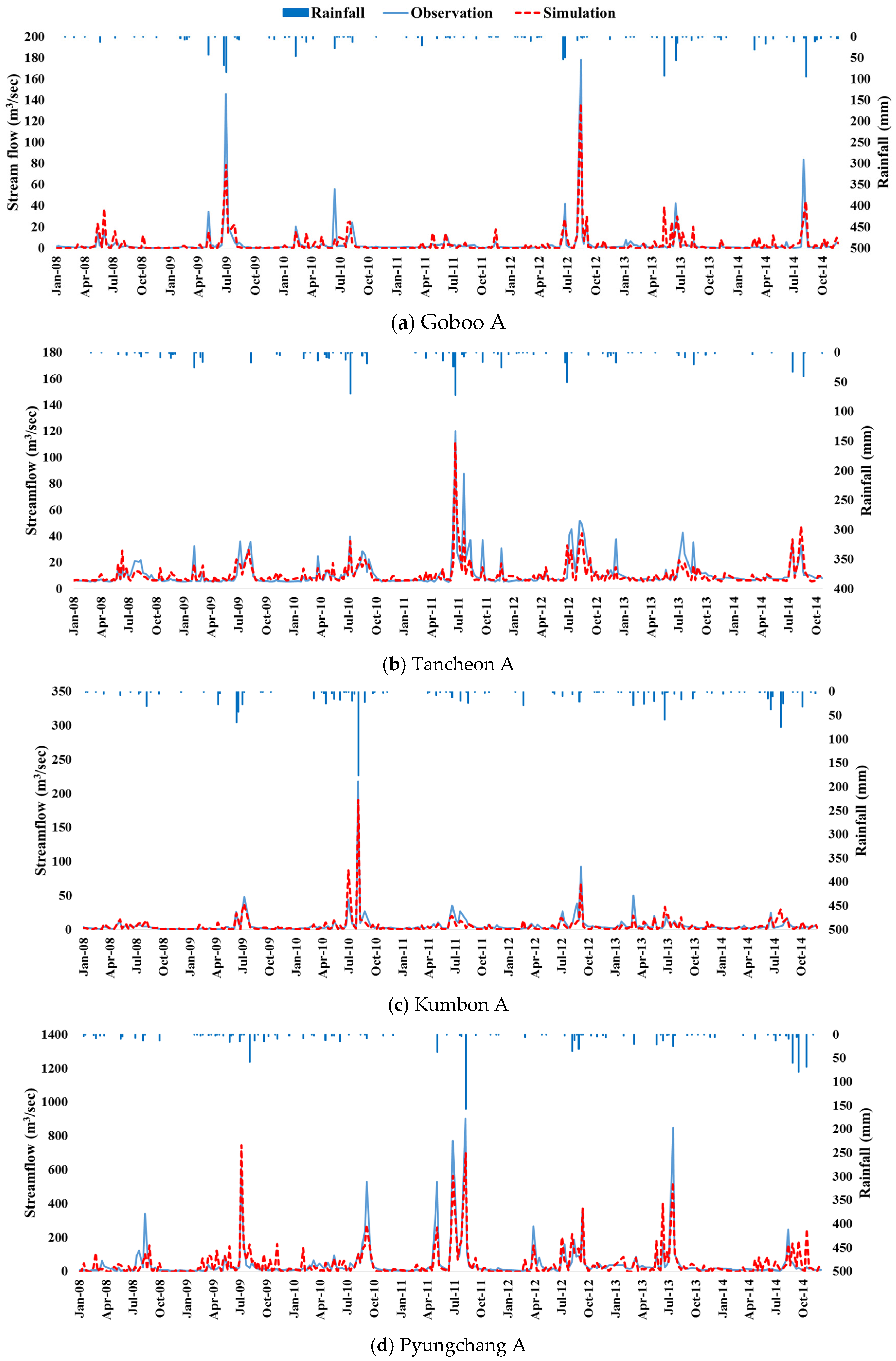
Comparisons of the simulation results and observed eight-day interval streamflows revealed reasonable agreement for the Goboo A watershed, with a coefficient of determination (R²) of 0.66 and Nash–Sutcliffe Efficiency (NSE) of 0.64. The R² values for Tancheon A, Kumbon A and Pyungchang A were 0.62, 0.9 and 0.62, respectively, and the NSE values were 0.61, 0.92 and 0.60, respectively (Figure 5 and

Table 7. Results of streamflow estimation and comparison of observed and estimated values. NSE, Nash–Sutcliffe Efficiency.

Watershed	Average Streamflow (2008–2010, Calibration)		R2	NSE	Average Streamflow (2011–2014, Validation)		R2	NSE
	Obs.	Est.			Obs.	Est.
Goboo A	4.45	3.92	0.66	0.64	4.13	4.48	0.79	0.78
Tancheon A	9.39	9.60	0.62	0.61	12.93	11.40	0.72	0.70
Kumbon A	5.95	6.09	0.93	0.93	6.34	5.92	0.62	0.60
Pyungchang A	34.38	36.74	0.62	0.60	53.69	51.35	0.80	0.79

).

The validation results for the Goboo A watershed indicated that the R² and NSE values were 0.79 and 0.78, respectively. The R² values for Tancheon A, Kumbon A and Pyungchang A were 0.72, 0.62 and 0.80, respectively, and the NSE values were 0.70, 0.60 and 0.79, respectively (Figure 5 and Table 7).

According to Ramanarayanan et al. [56] and Moriasi et al. [57], R² and NSE values that reflect satisfactory calibration of streamflow are R² ≥ 0.5 and NSE ≥ 0.5. By these criteria, the performance of the watershed-scale L-THIA ACN model developed in this study was acceptable, because the R² and NSE values obtained from the calibration and validation were greater than 0.6 for all four study watersheds considered (Table 7).

There were no significant differences in the average streamflow for the study watersheds. The differences between the observed data and simulated streamflows in the calibration were 11.9, 2.2, 2.4 and 6.9% for the Goboo A, Tancheon A, Kumbon A and Pyungchang A watersheds, respectively, and the differences in the validation were 8.5, 11.8, 6.6 and 4.4% (Table 7). As the results of this study show, the watershed-scale L-THIA ACN model can simulate streamflow well for watersheds ranging in size from 200.0 km²–1756.9 km².

As shown in Figure 5, the estimated peak flow during the high-flow season was lower than the observed peak flow. This can be explained by reduced infiltration, which is estimated using Equation (11). As the rainfall amount becomes greater, the CN estimated using the asymptotic CN approach becomes lower, resulting in a greater value of S (the potential maximum retention, mm). As S becomes greater, the infiltration approaches zero, especially for forest and pasture land covers. This results in a lower baseflow contribution to the total streamflow. Similar issues have been mentioned in other studies [58,59]. Although Equation (11) is simple to use in estimating the contributions of infiltration and baseflow to streamflow using the CN value, more in-depth investigation is needed to account for the lower infiltration that occurs in land cover areas with lower CN values.

4. Conclusions

In this study, LC-ACN-REs were improved by enabling consideration of HSG characteristics. In addition, a watershed-scale L-THIA ACN model was developed with direct runoff, baseflow and channel routing capabilities integrated together. With this new L-THIA model, users can simulate streamflow (direct runoff + baseflow) in a watershed. Daily rainfall data, land cover and HSG maps, DEM and ten additional model parameters are needed for the simulation of streamflow.

The simulated streamflow agreed well with the observed streamflow for the four study watersheds (as indicated by R² values in the range of 0.62–0.93 and NSE values in the range of 0.60–0.93 for both calibration and validation). These results demonstrate the predictive capability of the watershed-scale L-THIA ACN model developed in this study. Two model parameters (Adj_CN and DR_lag) were found to be closely related to the average field slope. Further in-depth investigation is needed to derive the relationships between the field slope length and these two model parameters. It should be noted that the watershed-scale L-THIA ACN model was not applied comprehensively to the watersheds for ranges of rainfall, land use, soil and topography conditions. It should also be noted that the values of the model parameters were estimated using manual calibration processes, which are affected by the subjective judgments of the model users.

For these reasons, automatic calibration using PARASOL (Parameter Solution), SUFI-2 (Sequential Uncertainty FItting algorithm), GLUE (Generalized Likelihood Uncertainty Estimation) and GA (Genetic algorithm) is needed for objective evaluation of the model parameters. With this function enabled, the relationship between the average field slope and the Adj_CN and DR_lag parameters could be analyzed and utilized in the watershed-scale L-THIA ACN model for streamflow estimation in ungaged watersheds.

References

1. Ma, F.; Ye, A.; Gong, W.; Mao, Y.; Miao, C.; Di, Z. An estimate of human and natural contributions to flood changes of the Huai River. Glob. PLanet. Change 2014, 119, 39–50. [Google Scholar] [CrossRef]
2. Yu, Q.; Wang, Y.; Xie, X.; Currell, M.; Pi, K.; Yu, M. Effects of short-term flooding on arsenic transport in groundwater system: A case study of the Datong Basin. J. Geochem. Explor. 2015, 158, 1–9. [Google Scholar] [CrossRef]
3. Stagge, J.H.; Kohn, I.; Tallaksen, L.M.; Stahl, K. Modeling drought impact occurrence based on meteorological drought indices in Europe. J. Hydrol. 2015, 530, 37–50. [Google Scholar] [CrossRef]
4. Logan, K.E.; Brunsell, N.A. Influence of drought on growing season carbon and water cycling with changing land cover. Agric. For. Meteorol. 2015, 213, 217–225. [Google Scholar] [CrossRef]
5. Martin, M.A.; Bourque, P.A. Mountain-river runoff components and their role in the seasonal development of desert-oases in northwest China. J. Arid Environ. 2015, 122, 1–15. [Google Scholar] [CrossRef]
6. Senaviratne, G.M.M.M.A.; Udawatta, R.P.; Anderson, S.H.; Baffaut, C.; Allen Thompson, A. Use of fuzzy rainfall-runoff predictions for clay pan watersheds with conservation buffers in Northeast Missouri. J. Hydrol. 2014, 517, 1008–1018. [Google Scholar] [CrossRef]
7. Lin, B.; Chen, X.; Yao, H.; Chen, Y.; Liu, M.; Gao, L.; James, A. Analyses of landuse change impacts on catchment runoff using different time indicators based on SWAT mode. Ecol. Indic. 2015, 58, 55–63. [Google Scholar] [CrossRef]
8. Holvoet, K.M.A.; Seuntjens, P.; Vanrolleghem, P.A. Monitoring and modeling pesticide fate in surface waters at the catchment scale. Ecol. Model. 2007, 209, 53–64. [Google Scholar] [CrossRef]
9. Jayakrishnan, R.S.R.S.; Srinivasan, R.; Santhi, C.; Arnold, J.G. Advances in the application of the SWAT model for water resources management. Hydrol. Proc. 2005, 19, 683–692. [Google Scholar] [CrossRef]
10. Gassman, P.W.; Reyes, M.R.; Green, C.H.; Arnold, J.G. The soil and water assessment tool: Historical development, applications, and future research directions. Trans. ASABE 2007, 50, 1211–1250. [Google Scholar] [CrossRef]
11. Meaurio, M.; Zabaleta, A.; Uriarte, J.A.; Srinivasan, R.; Antiguedad, I. Evaluation of SWAT models performance to simulate streamflow spatial origin. The case of a small forested watershed. J. Hydrol. 2015, 525, 326–324. [Google Scholar] [CrossRef]
12. Grimaldi, S.; Petroselli, A.; Serinaldi, F.A. Continuous Simulation Model for Design-Hydrograph Estimation in Small and Ungauged Watersheds. Hydrol. Sci. J. 2012, 57, 1035–1051. [Google Scholar] [CrossRef]
13. Grimaldi, S.; Petroselli, A.; Romano, N. Curve-Number/Green-Ampt mixed Procedure for Streamflow Predictions in Ungauged basins: Parameter Sensitivity Analysis. Hydrol. Proc. 2013, 27, 1265–1275. [Google Scholar] [CrossRef]
14. Arnold, J.G.; Moriasi, D.N.; Gassman, P.W.; Abbaspour, K.C.; White, M.J.; Srinivasan, R.; Santhi, C.; Harmel, R.D.; van Griensven, A.; Van Liew, M.W.; et al. SWAT: Model use, calibration and validation. Trans. ASABE 2012, 55, 1491–1508. [Google Scholar] [CrossRef]
15. Harbor, J. A practical method for estimating the impact of land use change on surface runoff. Groundwater Recharge and Wetland Hydrology. J. Am. Plan. Asssoc. 1994, 60, 91–104. [Google Scholar] [CrossRef]
16. Bhaduri, B.; Grove, M.; Lowry, C.; Harbor, J. Assessing the long-term hydrologic impact of land-use change: Cuppy McClure watershed, Indiana. J. Am. Water Works Assoc. 1997, 89, 94–106. [Google Scholar]
17. Lim, K.J.; Engel, B.A.; Tang, Z.; Muthukrishnan, S.; Choi, J.; Kim, K. Effects of calibration on L-THIA GIS runoff and pollutant estimation. J. Environ. Manag. 2006, 78, 35–43. [Google Scholar] [CrossRef] [PubMed]
18. U.S. Environmental Protection Agency (USEPA). SWMM 5 User’s Manual; EPA/600/R-05/040; National Risk Management Research Laboratory, Office of Research and Development: Cincinnati, OH, USA, 2010.
19. Gironas, J.; Roesner, L.A.; Rossman, L.A.; Davis, J.A. New applications manual for the Storm Water Management Model (SWMM). Environ. Model. Softw. 2010, 25, 813–814. [Google Scholar] [CrossRef]
20. Tetra Tech. User's Guide Spreadsheet Tool for the Estimation of Pollutant Load (STEPL), Version 4.1; Tetra Tech: Fairfax, VA, USA, 2011. [Google Scholar]
21. Park, Y.S.; Engel, B.A. A web-based model to estimate the impact of best management practices. Water 2014, 6, 455–471. [Google Scholar] [CrossRef]
22. Soil Conservation Service. (SCS). National Engineering Handbook; Section 4, Hydrology; US 444 Department of Agriculture, US Government Printing Office: Washington, DC, USA, 1972.
23. Engel, B.A. GIS-Based CN Runoff Estimation; Agricultural and Biological Engineering Departmental Report; Purdue University: West Lafayette, IN, USA, 1997. [Google Scholar]
24. Lim, K.J.; Engel, B.A.; Kim, Y.; Bhaduri, B.; Harbor, J. Development of the Long-Term Hydrologic Impact Assessment (L-THIA) WWW System. In Proceedings of the 10th International Soil Conservation, West Lafayette, IN, USA, 2 May 2002; Stott, D., Mohtar, R., Steinhardt, G., Eds.; Purdue University: West Lafayette, IN, USA, 2002; pp. 1018–1023. [Google Scholar]
25. Tang, Z.; Engel, B.A.; Lim, K.J.; Pijanowski, B.C.; Habor, J. Minimizing the Impact of urbanization on long term runoff. J. Am. Water Res. Assoc. 2005, 41, 1347–1359. [Google Scholar] [CrossRef]
26. Jang, C.H.; Kum, D.H.; Jung, Y.; Kim, K.; Shin, D.S.; Engel, B.A.; Shin, Y.; Lim, K.J. Development of a Web-based L-THIA 2012 direct runoff and pollutant Auto-calibration module using a genetic algorithm. Water 2013, 5, 1952–1963. [Google Scholar] [CrossRef]
27. Park, Y.S.; Lim, K.J.; Theller, L.; Engel, B.A. L-THIA GIS Manual; Agricultural and Biological Engineering Departmental Report; Purdue University: West Lafayette, IN, USA, 2013. [Google Scholar]
28. Ahiablame, L.M.; Engel, B.A.; Chaubey, I. Representation and evaluation of low impact development practices with L-THIA-LID: An example for site planning. Environ. Pollut. 2012, 1, 1–13. [Google Scholar] [CrossRef]
29. Ryu, J.; Jung, Y.; Kong, D.S.; Park, B.K.; Kim, Y.S.; Engel, B.A.; Lim, K.J. Approach of Land Cover based Asymptotic Curve Number Regression Equation to Estimate Runoff. J. Irrig. Drain. Eng. 2016. accepted. [Google Scholar]
30. Hawkins, R.H. Asymptotic determination of runoff curve numbers from data. J. Irrig. Drain. Eng. 1993, 119, 334–345. [Google Scholar] [CrossRef]
31. Tedela, N.M.; McCutcheon, S.C.; Rasmussen, T.C.; Hawkins, R.H.; Swank, W.T.; Campbell, J.L.; Adams, M.B.; Jackson, C.R.; Tollner, E.W. Runoff curve numbers for 10 small forested watersheds in the mountains of the eastern United States. J. Hydrol. Eng. 2012, 17, 1188–1198. [Google Scholar] [CrossRef]
32. Gundalia, M.; Dholakia, M. Impact of monthly curve number on daily runoff estimation for Ozat catchment in India. J. Mod. Hydrol. 2014, 4, 144–155. [Google Scholar] [CrossRef]
33. Banasik, K.; Woodward, D. Empirical determination of runoff curve number for a small agricultural watershed in Poland. In Proceedings of the 2nd Joint Federal Interagency Conference, Las Vegas, NV, USA, 27 June–1 July 2010.
34. Soulis, K.X.; Valiantzas, J.D.; Dercas, N.; Londra, P.A. Investigation of the Direct runoff Generation Mechanism for the Analysis of the SCS-CN method Applicability to a Partial area Experimental Watershed. Hydrol. Earth Syst. Sci. 2009, 13, 605–615. [Google Scholar] [CrossRef]
35. Soulis, K.X.; Valiantzas, J.D. SCS-CN parameter determination using rainfall-runoff data in heterogeneous watersheds—The Two-CN system approach. Hydrol. Earth Syst. Sci. 2012, 16, 1001–1015. [Google Scholar] [CrossRef]
36. Soulis, K.X.; Valiantzas, J.D. Identification of the SCS-CN Parameter Spatial Distribution using Rainfall-Runoff data in Heterogeneous Watersheds. Water Res. Manag. 2013, 27, 1737–1749. [Google Scholar] [CrossRef]
37. Ryu, J.; Kim, E.J.; Han, M.D.; Kim, Y.S.; Kum, D.H.; Lim, K.J.; Park, B.K. Enhancement of Estimation Method on the Land T-P Pollutant Load in TMDLs Using L-THIA. J. Korean Soc. Environ. Eng. 2014, 36, 162–171. [Google Scholar] [CrossRef]
38. Neitsch, S.L.; Arnold, J.G.; Kiniry, J.R.; Williams, J.R. Soil & Water Assessment Theoretical Documentation Version 2005; Soil and Water Research Lavatory, Agricultural Research Service: Temple, TX, USA, 2005. [Google Scholar]
39. Huang, M.; Gallichand, J.; Wang, J.; Goulet, M. A modification to the Soil Conservation Service curve number method for steep slopes in the Loess Plateau of China. Hydrol. Proc. 2006, 20, 579–589. [Google Scholar] [CrossRef]
40. Grimaldi, S.; Petroselli, A.; Tauro, F.; Porfiri, M. Time of concentration: A paradox in modern hydrology. Hydrol. Sci. J. 2012, 57, 217–228. [Google Scholar] [CrossRef]
41. Hulsman, P. Determination of the Main Areas Contributing to the Suspended Sediment Load in the Mara River, Kenya. Master’s Thesis, National University of Singapore, Singapore, 2015. [Google Scholar]
42. Engman, E.T. Roughness coefficient for routing surface runoff. J. Irrig. Drain. Eng. 1986, 112, 39–53. [Google Scholar] [CrossRef]
43. Hickey, R. Slope angle and slope length solutions for GIS. Cartography 2000, 29, 1–8. [Google Scholar] [CrossRef]
44. Petroselli, A. LIDAR data and Hydrological Applications at the basin scale. GISci. Remote Sens. 2012, 49, 139–162. [Google Scholar] [CrossRef]
45. Wischmeier, W.H.; Smith, D.D. Predicting Rainfall Erosion Losses: A Guide to Conservation Planning. USDA Agricultural Handbook; No. 537; U.S. Gov. Print. Office: Washington, DC, USA, 1978.
46. Dingman, S.L. Physical Hydrology; Prentice-Hall, Inc.: Englewood Cliffs, NJ, USA, 1994. [Google Scholar]
47. Arnold, J.G.; Allen, P.M.; Bernhardt, G.A. Comprehensive surface groundwater flow model. J. Hydrol. 1993, 142, 47–69. [Google Scholar] [CrossRef]
48. Venetis, C. A study of the recession of unconfined aquifers. Bull. Int. Assoc. Sci. Hydrol. 1969, 14, 119–125. [Google Scholar] [CrossRef]
49. Sangrey, D.A.; Harrop-Williams, K.O.; Klaber, J.A. Predicting groundwater response to precipitation. J. Geotechnol. Geoenviron. Eng. 1984, 110, 957–975. [Google Scholar] [CrossRef]
50. Kim, H.W.; Sin, Y.J.; Choi, J.H.; Kang, H.W.; Ryu, J.; Lim, K.J. Estimation of CN-based infiltration and baseflow for effective watershed management. J. Korean Soc. Water Environ. 2011, 27, 405–412. [Google Scholar]
51. Hooghoudt, S.B. Bijdrage tot de kennis van enige natuurkundige grootheden van de ground. Versl. Landbouwkd. Onderz. 1940, 46, 515–707. [Google Scholar]
52. Smedema, L.K.; Rycroft, D.W. Land Drainage: Planning and Design of Agricultural Systems; Batsford Academic and Educational Ltd: London, UK, 1983. [Google Scholar]
53. Cunge, J.A. On the subject of flood propagation method (Muskingum method). J. Hydraul. Res. 1969, 7, 205–230. [Google Scholar] [CrossRef]
54. Boroughs, C.B.; Zagona, E.A. Daily flow routing with the Muskingum-Cunge method in the Pecos River Ware Model. In Proceedings of the Second Federal Interagency Hydrologic Modeling Conference, Las Vegas, NV, USA, 29 July–1 August 2002.
55. Williams, J.R. Flood routing with variable travel time or variable storage coefficients. Trans. ASAE 1969, 12, 100–103. [Google Scholar] [CrossRef]
56. Ramanarayanan, T.S.; Williams, J.R.; Dugas, W.A.; Hauck, L.M.; McFarland, A.M.S. Using APEX to identify alternative practices for animal waste management. In Proceedings of the American Society of Agricultural Engineers Annual International Meeting, Minneapolis, MN, USA, 10–14 August 1997.
57. Moriasi, D.N.; Arnold, J.G.; VanLiew, M.W.; Bingner, R.L.; Hrmel, R.D.; Veith, T.L. Model evaluation guidelines for systematic quantification of accuracy in watershed simulations. Trans. ASABE 2007, 50, 885–900. [Google Scholar] [CrossRef]
58. Mishra, S.K.; Singh, V.P. Validity and extension of the SCS-CN method for computing infiltration and rainfall-excess rates. Hydrol. Proc. 2004, 18, 3323–3345. [Google Scholar] [CrossRef]
59. Tyagi, J.V.; Mishra, S.K.; Singh, R.; Singh, V.P. SCS-CN based time-distributed sediment yield model. J. Hydrol. 2008, 352, 388–403. [Google Scholar] [CrossRef]
Figure 1. Asymptotic CN regressions obtained in the study by Hawkins [30]. CN(P) is the Curve Number as a function of rainfall, and CN0 = 100/(1 + P/2) defines a threshold below which no runoff occurs until the rainfall P in mm exceeds an initial abstraction of 20% of the maximum potential retention.
Water 08 00153 g001
Figure 2. Flow diagram for the development of watershed-scale L-THIA ACN model.
Water 08 00153 g002
Figure 3. Storage in a river reach versus reach outflow [54].
Water 08 00153 g003
Figure 4. Four study watersheds for evaluation of watershed-scale L-THIA ACN model.
Water 08 00153 g004
Figure 5. Results of estimation of streamflow (2008–2014, eight-day interval).
Water 08 00153 g005