Abstract
The hydrodynamic characteristics of a delta or estuary are mainly governed by discharges of rivers and water level at the sea (or lake) boundaries. A joint probability approach is widely applied to quantify the high water level frequency in deltas. In the approach the relevant hydrodynamic loading variables, namely the astronomical tides, the wind induced storm surge and the river flows, are jointly investigated. The joint probability distribution is used to generate a large number of scenarios of boundary conditions which can drive a deterministic model to derive the water levels at locations of interest. The resulting water levels as well as their associated joint probabilities can be inverted to the high water level frequency curve. However, in the joint probability distribution, marginal distributions may contain large statistical uncertainties due to their relevant parameters being estimated from a limited length of data. In the case of the Rhine Delta, a nonparametric bootstrap method is applied to quantify the statistical uncertainties in three critical marginal distributions: wind induced storm surge peak level, wind induced storm surge duration and River Rhine discharge. The uncertainties are incorporated into the marginal distributions with a Monte Carlo integration method. Further the uncertainty-incorporated marginal distributions are used for the high water level frequency assessment. Compared to previous studies, water levels for given return periods are much higher. The uncertainty differs in each marginal distribution and its impact on the high water level frequency curve also varies.
1. Introduction
The hydrodynamic characteristics of a delta or estuary are mainly governed by discharges of rivers and water levels at sea (or lake) boundaries. The joint probability approach is widely used to quantify the high water level frequency in deltas [1,2,3,4,5,6,7]. In the Rhine Delta, the relevant hydrodynamic loading variables at boundaries, namely the astronomical tides, the wind induced storm surges and the river flows, are jointly investigated and their joint probability distribution is estimated from the historical flood events [7]).
The high water level frequency assessment consists of two steps: first, a large number of stochastic scenarios of extreme boundary conditions are generated from the joint probability distribution; second, these generated scenarios are used as inputs to drive a deterministic hydrodynamic model to result in the peak water levels at locations of interest in the delta. The resulting peak water levels can be converted to the high water level frequency curve. The probabilistically computed high water level frequency is critically influenced by the joint probability distribution, time evolution of the relevant loading variables and accuracy of the hydrodynamic model.
In the joint probability approach, to get the marginal distributions (Rhine flood, wind induced storm surges), the annual maximal value during the observed year is determined and then a distribution to this series of annual maxima is fitted. From the obtained distribution, a flood event with a certain return period can be estimated. In general two different sources of uncertainty exist in this process [8]. Natural uncertainty refers to the variability of the flood events, mostly due to the limited number of flood events. For example, to estimate a 1000-year flood event based on a few dozen years flood records. Epistemic uncertainty consists of two parts: the uncertainty in distribution type chosen and in the parameter estimation. In this article, we focus on this natural uncertainty.
Statistical uncertainty exists in the marginal distributions of the joint probability distribution, which refers to the uncertainty in the parameters of the marginal distributions caused by estimating them from a limited number of flood events.And this is what we have to work with. Hence, better assessment of the statistical uncertainty due to insufficient data would be helpful.
The nonparametric bootstrap method is that from the given sample, new samples are generated by using resampling with replacement [9,10,11]. It relies on re-sampling with replacements from the given observations and providing estimates of uncertainty of distribution variables and quantiles. It is employed to quantify the natural uncertainty in the distributions as it is simple to present and easy to implement [12,13,14]
The statistical uncertainty can be incorporated in the marginal distributions to form new marginal distributions by a Monte Carlo integration method. It is expected that the new distributions will increase the probability of extreme load values because of the uncertainty in the low quantiles of the marginal distributions. In the joint probability distribution, the marginal distributions with/without incorporating the statistical uncertainty are applied to probabilistically compute the high water level frequency curve. Then the impact of the statistical uncertainty of the marginal distributions on the high water level frequency curve can be investigated and quantified.
This study briefly introduces the joint probability approach to assess the high water level frequency in the Lower Rhine Delta, and aims to quantify the statistical uncertainty in the marginal distributions, and further evaluate the impact on the high water level frequency. This article will specifically focus on the case of the Lower Rhine Delta. It is organized as follows: Section 2 presents the method; the case is shown in Section 3; followed by the conclusion in Section 4.
2. Methods
The outline of the method is illustrated in Figure 1. First, the bootstrap method is applied to estimate statistical uncertainty in the marginal distributions. Second, the statistical uncertainty is incorporated into the marginal distributions to form into new marginal distributions. Third, the new marginal distributions are applied to compute the high water level frequency in the Lower Rhine Delta, and to assess the impact of statistical uncertainty on the high water level frequency.
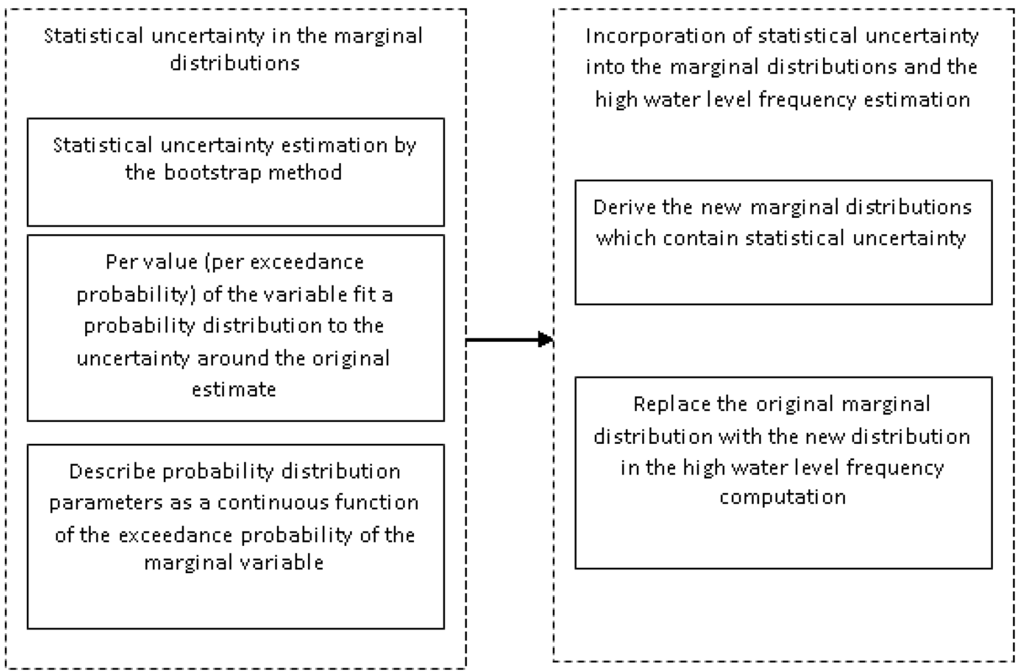
Figure 1.
Outline of the method.
2.1. Statistical Uncertainty in a Distribution
The statistical uncertainty in a distribution can be estimated using the nonparametric bootstrap method, and subsequently parameterized as a probability distribution function of the exceedance probability of the variable.
The nonparametric bootstrap method generates a predetermined N samples of the variable by randomly re-sampling with replacement from the original sample. Each generated sample has the same size of the original sample. Each sample fits to a same probability distribution, and then there are N distributions. For a given exceedance probability of the variable, around the original estimate there are N values derived from the N distributions. These N values can fit to a distribution. For example, the log-normal distribution, a simple skewed distribution can be chosen.
The probability density function of a log-normal distribution is:
u and are the location parameter and the scale parameter on a logarithmic scale respectively.
The log-normal parameters can be made continuous functions of the exceedance probability of the variable. The parameter can be modeled as a function of the exceedance probability P by fitting a polynomial.
The mode of the log-normal distribution is the value with maximum probability density. The original estimate of the variable x is assumed to serve as the mode of the log-normal distribution, see Equation (2), and therefore the other log-normal parameter u can be estimated from Equation (3):
here P is the exceedance probability of the marginal variable.
The statistical uncertainty in the distribution can be estimated by the Log-normal distribution: given a value of x, the corresponding Log-normal distribution, in terms of the parameters u and , around that x is known.
2.2. Uncertainty-Incorporated Distribution
The statistical uncertainty can be incorporated into the distribution according to Equation (4) by the Monte Carlo Integration method. In Equation (4), x is the original variable, is the uncertainty value and xun is the uncertainty incorporated variable, where .
here Fun (xun) is the uncertainty incorporated distribution of the variable; fx is the original distribution of the variable; Flogn is the Log-normal (statistical uncertainty) distribution conditioned on x.
2.3. Impact of the Uncertainty on the High Water Level Frequency in the Rhine Delta
The hydrodynamic characteristics of the Rhine Delta are mainly governed by discharges of the Rhine and Meuse and the water level at the North Sea boundaries, as can be seen in Figure 2 and Figure 3. A joint probability approach using a 1-D hydrodynamic model was applied to assess the high water level frequency in the Lower Rhine Delta [7]. The operational control of the existing flexible hydraulic structures (red points in Figure 4) was taken into account.
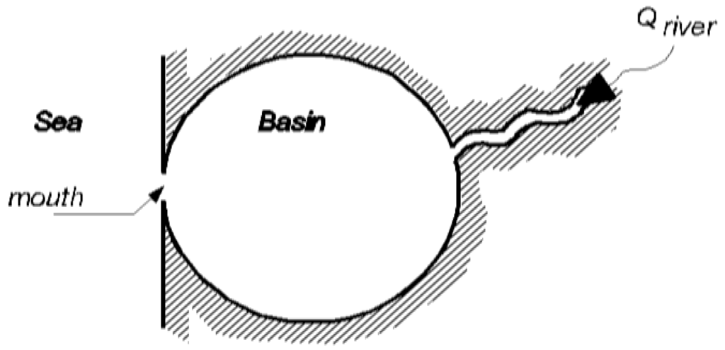
Figure 2.
The conceptual model of the open delta.

Figure 3.
The conceptual model of the closable delta.
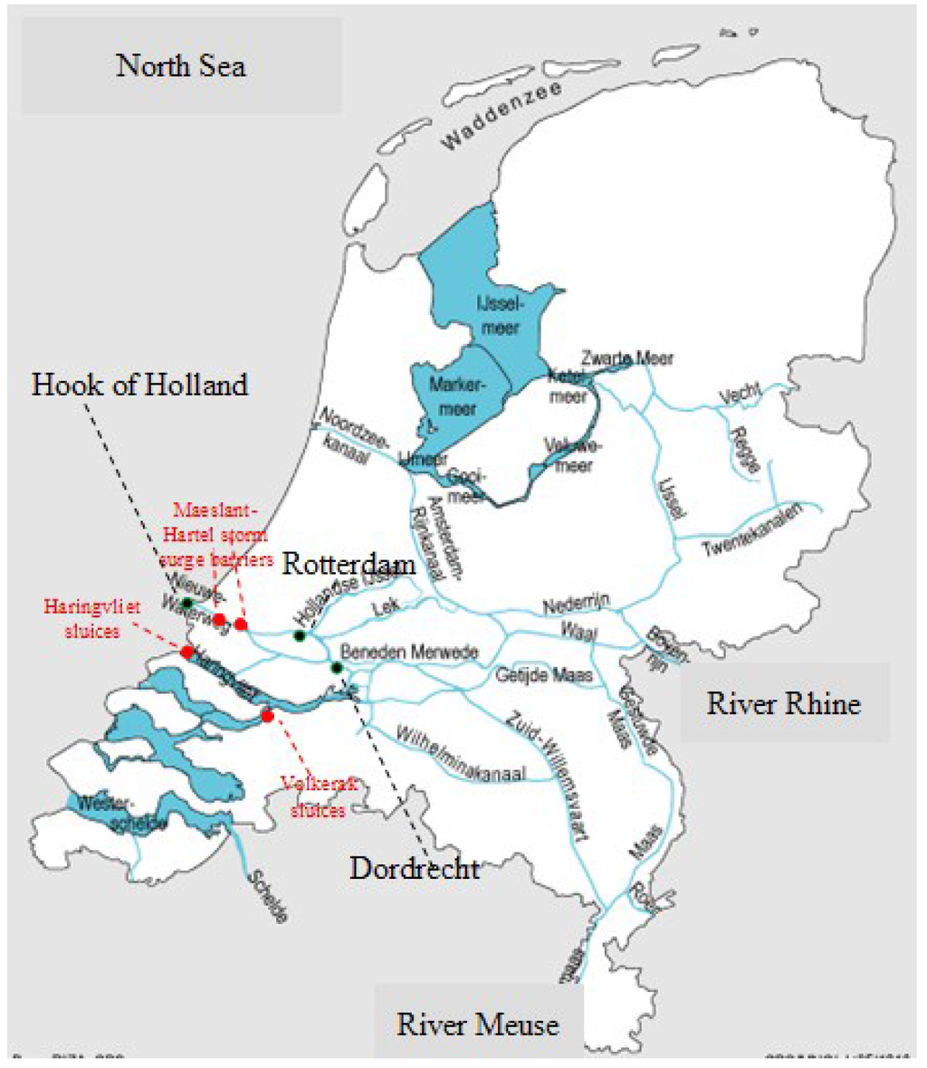
Figure 4.
The Rhine Delta with operated hydraulic structures [19,20].
To reduce the computation burden, A conceptual model, the “Equal Level Curves” [15,16] is preferred to be applied to examine the interaction of sea level, fluvial flows and infrastructure operations to produce water levels at locations of interest in the Rhine Delta. Equal Level Curves are a simple steady state function, which can simulate the highest water level at Rotterdam by boundary conditions during one tidal period.
Two states of Equal Level Curves are introduced, see Figure 2 and Figure 3: one for the open delta where all dams and barriers are open, and the other for the closable delta where all dams and barriers along the coast are closed. This model has advantages: first, less information needed and a strong reduction in computation time; second, convenient to combine with the present operation control of the Maeslant storm surge barrier at the mouth of the delta. More information is in Appendix A.
According to previous studies [7,16,17], particular attention is paid to the simultaneous occurrence of storm surges and Rhine floods. Facing this kind of flood event, the Haringvliet dam gates and the Maeslant Storm Surge Barrier with the Hartel Storm Surge Barrier should be closed to protect high sea levels from propagating into the delta [18,19,20], but unfortunately the simultaneous high Rhine flow accumulating in a long closure duration can result in extreme high water level behind the dams and barriers.
In the joint probability of this kind of flood events, it is commonly assumed that the magnitude of the Rhine flow is independent of the magnitude of the storm surge [7,21,22,23] found no significant dependence of simultaneous occurrence of storm surges and Rhine floods. The marginal distributions were estimated from the selected flood events (Peak over Threshold values) with the parametric distributions (for example, generalized Pareto distribution). All parameters in the marginal distributions were estimated by the Maximum likelihood method. The joint probability distribution of this kind of event and its marginal distributions are shown in the Appendix B. The statistical uncertainty of three critical marginal distributions in terms of the wind induced storm surge peak level hsmax, the wind induced storm surge duration Ts and the high Rhine flow Qr, are discussed.
The flood risk map of the Netherlands indicated the urbanized areas Rotterdam and Dordrecht are more hazardous and vulnerable than other places in the Netherlands, and with the higher fatalities [24]. As a result, Rotterdam is taken as the study areas of interest for the high water level frequency estimation.
In the joint probability distribution, three marginal distributions with/without incorporating the statistical uncertainties are applied to compute the high water level frequency in Rotterdam. Thus, the impact of the statistical uncertainty on the high water level frequency can be investigated and quantified.
3. Results
3.1. Statistical Uncertainty
For each marginal variable, 1000 bootstrap samples are generated and fitted to 1000 bootstrap curves. Of which 41 curves (by order 25th, 50th ..., 475th, 525th ..., 950th, 975th, as well as 5th and 995th) are selected, shown as blue lines in Figure 5. The exceedance probability curve estimated by the original samples is shown in the red line in Figure 5. For a given exceedance probability of a marginal variable, 41 bootstrap estimates around the original estimate are fitted to a Log-normal distribution, as can be seen in Figure 6. Here only the figures with regard to the wind induce surge peak (hsmax) are given.
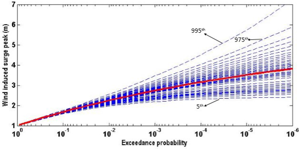
Figure 5.
Selected bootstrap quantiles for wind induced surge hsmax.
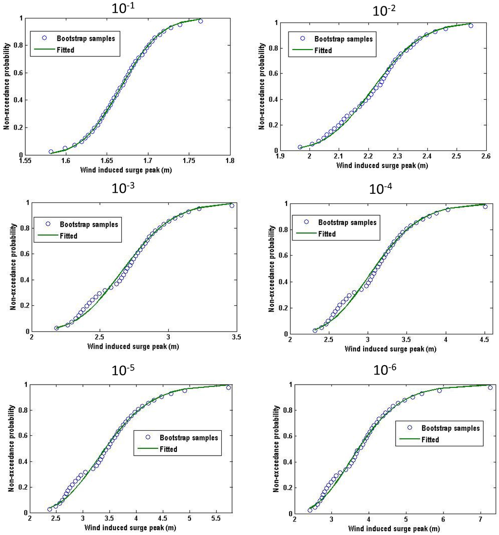
Figure 6.
The fitted Log-normal distributions at the exceedance probability of 10−1, 10−2, 10−3, 10−4, 10−5, 10−6 of wind induced surge hsmax.
The Log-normal parameters can be made continuous functions of the exceedance probability of the marginal variables. The estimated log-normal parameter for the exceedance probability is shown in Figure 7. The parameter can be modeled as a third-degree polynomial of the exceedance probability in Equation (5) in the region shown.
here P is the exceedance probability of the marginal variable, a1, a2, a3, a4 are the parameters estimated by fitting a polynomial with the method of least squares. The estimates of a1, a2, a3 and a4 for each marginal variable are shown in Table 1.
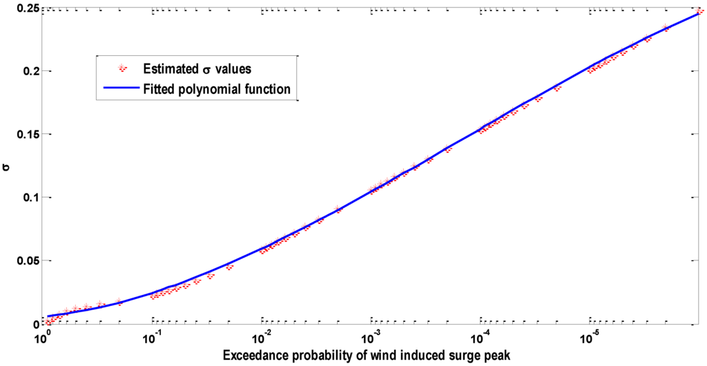
Figure 7.
The Log-normal distribution’s parameter σ is modeled as a function of the exceedance probability of the wind induced surge hsmax.

Table 1.
The estimates of a1, a2, a3 and a4 for the exceedance probabilities of each marginal variable.
The other Log-normal parameter u can be estimated based on Equation (3).
3.2. Uncertainty-Incorporated Marginal Distributions
Through application of Equation (4), the statistical uncertainties can be incorporated into the marginal distributions. The results are shown in Figure 8, Figure 9 and Figure 10.
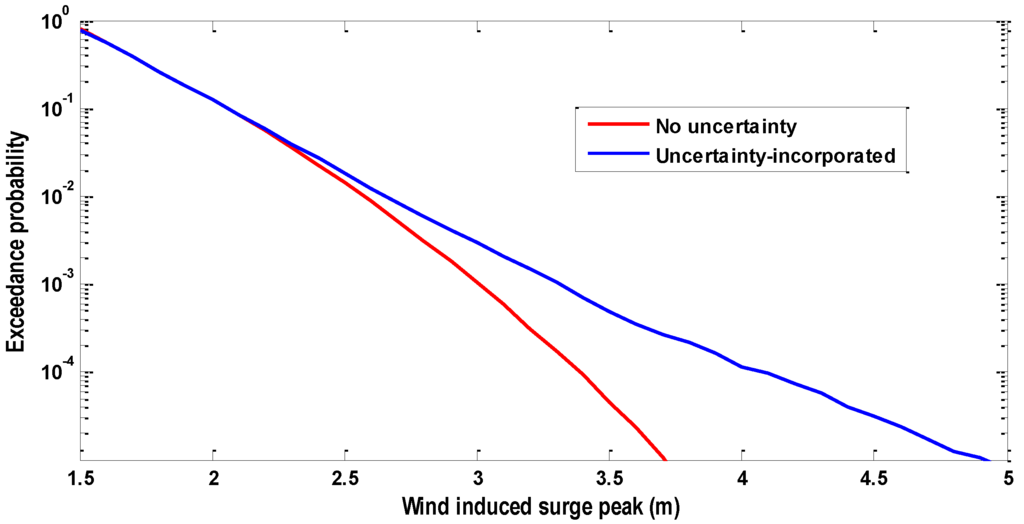
Figure 8.
The uncertainty-incorporated marginal distribution of the wind induced surge hsmax.
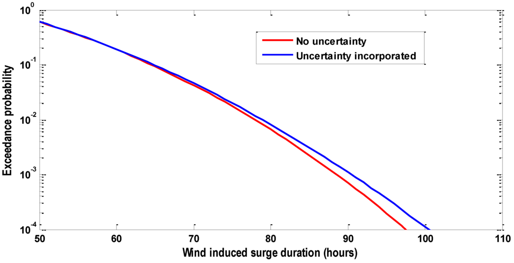
Figure 9.
The uncertainty-incorporated marginal distribution of the wind induced storm surge duration Ts.
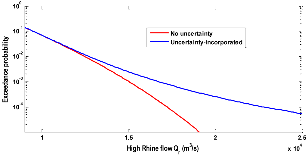
Figure 10.
The uncertainty-incorporated marginal distribution of the high Rhine flow Qr.
For higher exceedance probabilities (lower return periods), the uncertainty has a negligible effect on the uncertainty-incorporated distribution, mainly due to the small variance of the uncertainty for higher exceedance probabilities (see Figure 7). For lower exceedance probabilities (higher return periods), the variance increases, and the effect on the distributions becomes more substantial.
The results indicate that uncertainty incorporated marginal distributions result in more extreme values of the marginal variables at low exceedance probabilities.
However, considering the physical conditions the statistical uncertainty in the marginal distributions needs to be constrained at extreme return periods in order to avoid unreal situations.
3.3. Impact on the High Water Level Frequency
The impact of the statistical uncertainty on the high water level frequency can be addressed by the differences between the high water level frequency curves derived from two types of marginal distributions, as indicated in Section 2.3. The results are shown in Figure 11, Figure 12 and Figure 13 respectively.
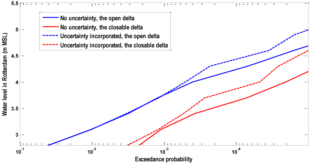
Figure 11.
The high water level frequency curve considering the statistical uncertainty in the marginal distribution of the wind induced surge hsmax.
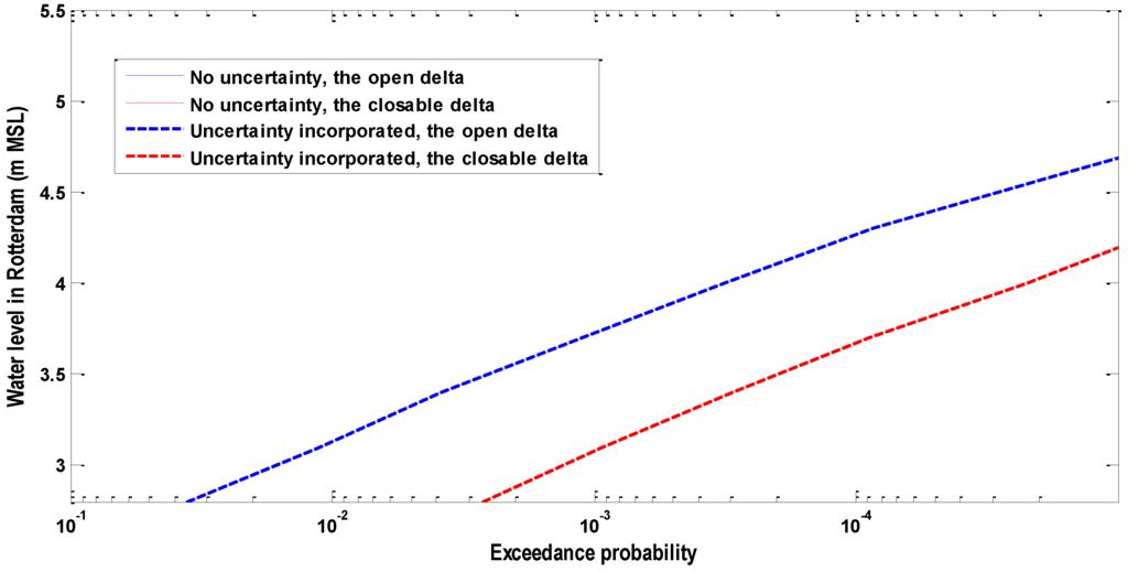
Figure 12.
The high water level frequency curve considering the statistical uncertainty in the marginal distribution of the wind induced storm surge duration Ts.
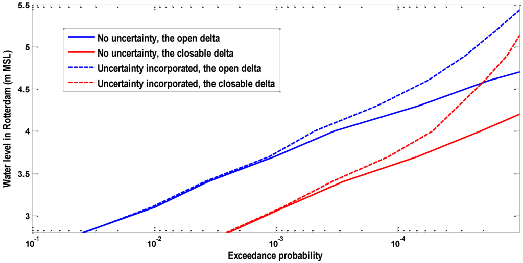
Figure 13.
The high water level frequency considering the statistical uncertainty in the above two marginal distributions.
In Figure 11, the high water level frequency curves in Rotterdam are estimated from two different marginal distributions of hsmax respectively. Incorporating the statistical uncertainty in the marginal distribution of hsmax significantly increases the high water level frequency in Rotterdam for the exceedance probabilities lower than 10−3.
In Figure 12, incorporating the statistical uncertainty in the marginal distribution of Ts does not affect the high water level frequency in Rotterdam.
In conclusion, the statistical uncertainty in each marginal distribution differs and its impact on the high water level frequency also varies.
In Figure 13, incorporating the statistical uncertainty in two marginal distributions significantly increases the high water level frequency in Rotterdam. Generally for higher exceedance probabilities (lower return periods), the statistical uncertainty has a negligible effect on the high water level frequency, while for lower exceedance probabilities (higher return periods), the effect on the high water level frequency becomes more substantial.
The design water level in Rotterdam is regarded as the water level with an exceedance frequency of 1/10,000; and its present value is 3.60 m above mean sea level (in brief MSL) [25]. As can be seen in Figure 12, the design water level of Rotterdam corresponds to 3.60 m MSL without considering the statistical uncertainty in three marginal distributions, while it corresponds to 3.75 m with considering the statistical uncertainty in three marginal distributions.
4. Conclusions and Recommendations
Quantifying high water level frequency is critical but complex in deltas or estuaries. In this article, the joint probability approach using a deterministic hydrodynamic model is applied to estimate the high water level frequency. This study aims at investigating statistical uncertainty of marginal distributions of the joint probability distribution and its impact on the high water level frequency. In the Rhine Delta, the results show that incorporating the statistical uncertainty in the marginal distributions will increase the high water level frequency because the probability of extreme hydraulic boundary conditions increases. The statistical uncertainty in each marginal distribution differs and its impact on the high water level frequency also varies.
Generally only a limited amount of data available when calculating the high water level frequency or flood frequency, however, this is what we have to work with. Hence, better assessment of the statistical uncertainty due to insufficient data would be helpful. In condition, considering real physical conditions, this statistical uncertainty should be constrained. For example, Rhine discharges in Lobith and sea levels in Hook of Holland have an physical upper limit. This constrain should be elaborated in future research.
Acknowledgments
We appreciate financial supports from National Natural Science Foundation of China (51479222, 41471427, 41101510) , the 111 Project (B08048).
Author Contributions
Hua Zhong and Pieter van Gelder designed this study and wrote this article; Wen Wang contributed to the statistical uncertainty analysis; Gaoxu Wang, Yongzhi Liu and Shuai Niu assised data analysis and drew the conclusions . All authors have read and approved the final manuscript.
Conflicts of Interest
The authors declare no conflict of interest
Appendix A
The Conceptual Model of the Rhine Delta
Considering the characteristics of the Rhine Delta, the conceptual model is illustrated. Two states of Equal Level Curves are introduced: one for the open delta where all dams and barriers are open, and the other for the closable delta where all dams and barriers along the coast are closed, as can be seen in Figure A1 and Figure A2. The closable delta can be open to the sea except that the delta can be closed with the help of hydraulic structures during the extreme weather conditions (storm surges). The conceptual model of the Lower Rhine Delta was introduced in Zhong et al. [16].
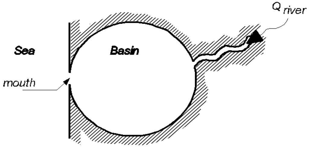
Figure A1.
The conceptual model of the open delta.
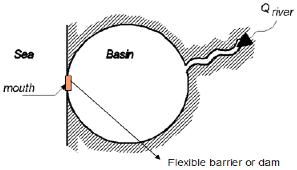
Figure A2.
The conceptual model of the closable delta.
Equal Level Curves are a simple steady state function, which can simulate the highest water level at Rotterdam by boundary conditions during one tidal period. For the open delta, Rotterdam water levels can be modeled by the Equal Level Curves with the boundary conditions of the Rhine flow at Lobith and the sea level at Hook of Holland, see Equation (A1):
here hR is the water level at Rotterdam; while hhvh stands for the sea water level at Hook of Holland. Qr is the Rhine flow at Lobith, and Qr is the Meuse flow at Borgharen. is the discharge coefficient, A stands for the surface area of the cross section in Hook of Holland and g is the gravitational acceleration. The parameters of and A can be estimated by the linear regression method with the selected historical flood event, and is estimated to be 3620 m2.
here h0 is the mean sea level, ha is the astronomical tide level, hs is the wind induced surge level. From a statistical point of view, the occurrence of the astronomical tide component is independent of the occurrence of the wind induced storm surge component at the mouth of the Rhine Delta. However, these two components can interact with each other when they propagate into the delta. Their nonlinear interaction generally increases the surge height at a rising astronomical tide and decreases the surge height at a high astronomical tide. Quantifying the nonlinear effect is beyond the scope of this study. For the sake of convenience, it can be assumed that the wind induced storm surge is independent of the astronomical tide.
Equal Level Curves with the open delta are shown in Figure A3.
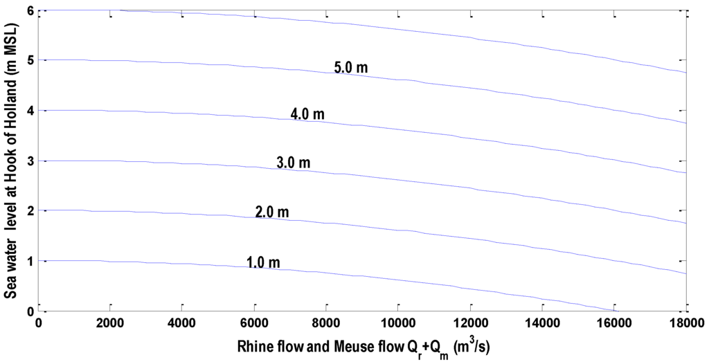
Figure A3.
Equal Level Curves with the open delta at Rotterdam.
At present, the Rhine delta can be kept open always via the New Waterway and be closed by closing the Maeslant Barrier and the Haringvliet dams when facing storm surges.
Being a closable delta, there are two states for the Equal Level Curves: the state of open can be described by Equation (A1), the state of closure can be described by Equation (A3). After the closure of the delta, the water level behind the barrier rises because the Rhine flow cannot be discharged into the North Sea and will accumulate. In this process the heights of the surrounding dikes are assumed to be infinite high and no dike breaches occur.
where hR is Rotterdam water level after the closure duration ΔT; hR,c is the average water level behind the Maeslant barrier at the closure time; Qr is the Rhine flow at Lobith; Qm is the Meuse flow at Borgharen; B is the surface area of the delta where water can be stored.
hr,c can be estimated from the average water level of four locations (Rotterdam, Goidschalxoord, Dordrecht, and Moerdijk) at the moment of the Maeslant barrier closing.
The water levels at these four locations at time t depend on the sea water level of a few hours ago at Hook of Holland and on the Rhine and Meuse discharges of 24 hours ago at Lobith and Borgharen. The functions are shown in Equations (A4)–(A7). The parameters of the below equations are estimated from system identification of historical measurements. The time unit of t is an hour.
The parameter B can be estimated by inverting Equation (A3) into:
The factor 8/9 comes from the distribution of the Rhine River inflow of which 1/9 flows north towards the IJsselmeer. The water level can rise by Δh after the closure time ΔT. In the closure event of 2007, the Rhine discharge Qr was 1171 m3/s, the Meuse discharge Qm was 148 m3/s and the water level at Rotterdam rose from 0.70 to 1.12 m after 15 hours closure. In Figure A4, the derivative is constant and the value of B is estimated to be 152 km2.
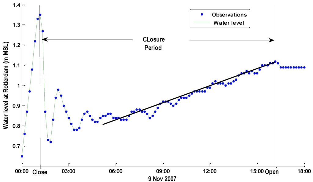
Figure A4.
Rotterdam water level during the first closure event of 9 November 2007.
The closure duration ΔT depends on the operational control of closing and opening of the delta. Two hydraulic structures: the Maeslant storm surge barrier and the Haringvliet dams are mainly responsible for closing the Rhine delta. When a high Rhine flow coincides with a storm surge, the present operational control of the Haringvliet dams keep the Rhine delta partly open, depending on the quantity of the Rhine flow in Lobith. However, to keep the analysis simple, it is assumed that when the Maeslant Barrier closes, the Haringvliet dams fully close. This assumption will overestimate the water level when a storm surge coinciding with a high Rhine flow occurs. Therefore, the closure duration ΔT depends on the operational control of the Maeslant Barrier responding to the hydraulic boundary conditions.
The control system of the Maeslant Barrier (named BOS, in Dutch: Beslissing & Ondersteunend Systeem; in English, Decision and Support System) has the responsibility to close the barrier completely autonomously [18]. To keep the analysis simple, it is assumed that only one control parameter is considered: the closing decision level Hd, in the operational control of the barrier. When Rotterdam water level is predicted to exceed the closing decision level Hd (3.0 m MSL in Rotterdam), the barrier is assumed to close at two hour before. In reality, the barrier closes at the moment the current starts to change from seaward direction to landward direction, however, to calculate this moment needs extra information which is not the main concern in this article. The water level in Hook of Holland drops after the storm surge, and when the water level in Rotterdam is higher than the water level in Hook of Holland, the barrier re-opens. Considering the time the procedure of close and re-open takes, the minimum closure duration is 6 hours. The closure decision making of the Maeslant Barrier is illustrated in Figure A5.
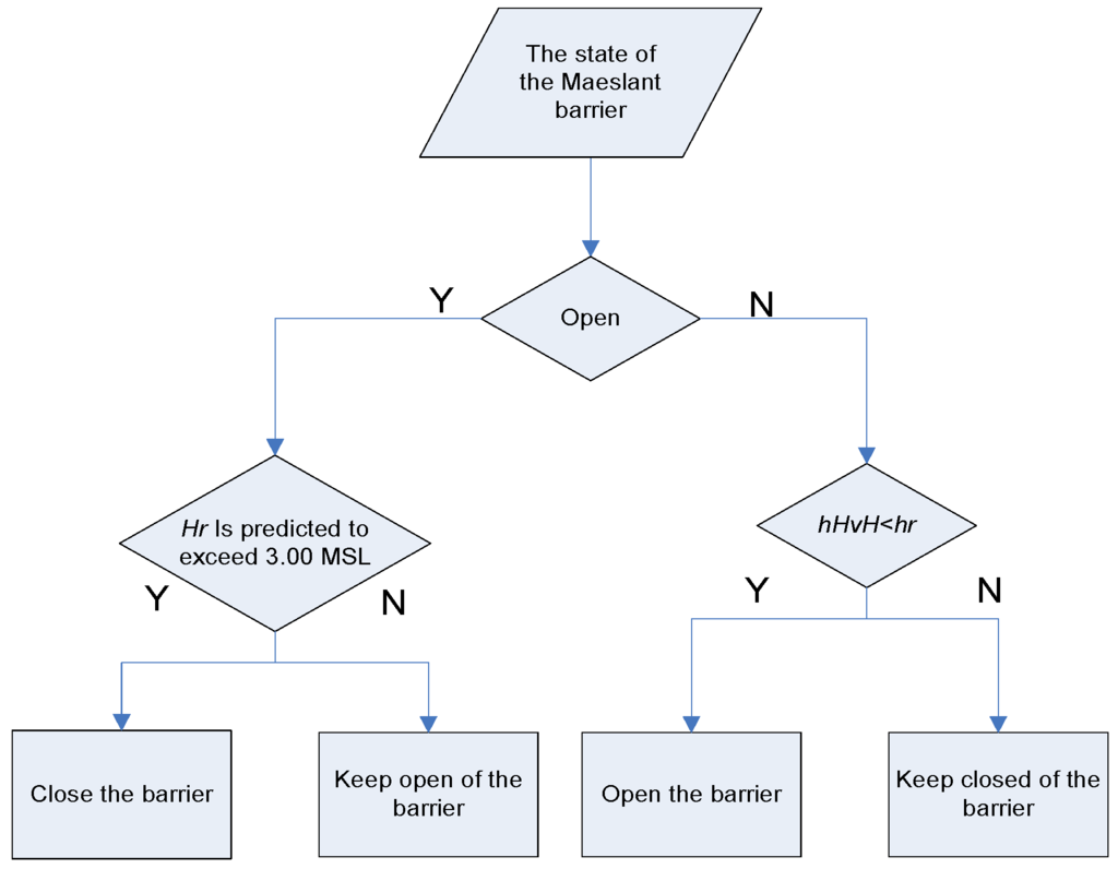
Figure A5.
The closure decision making of the Maeslant Barrier.
Equal Level Curves for the closable delta are shown in Figure A6 in which Equal Level Curves in the shaded area are presented in Figure A7.
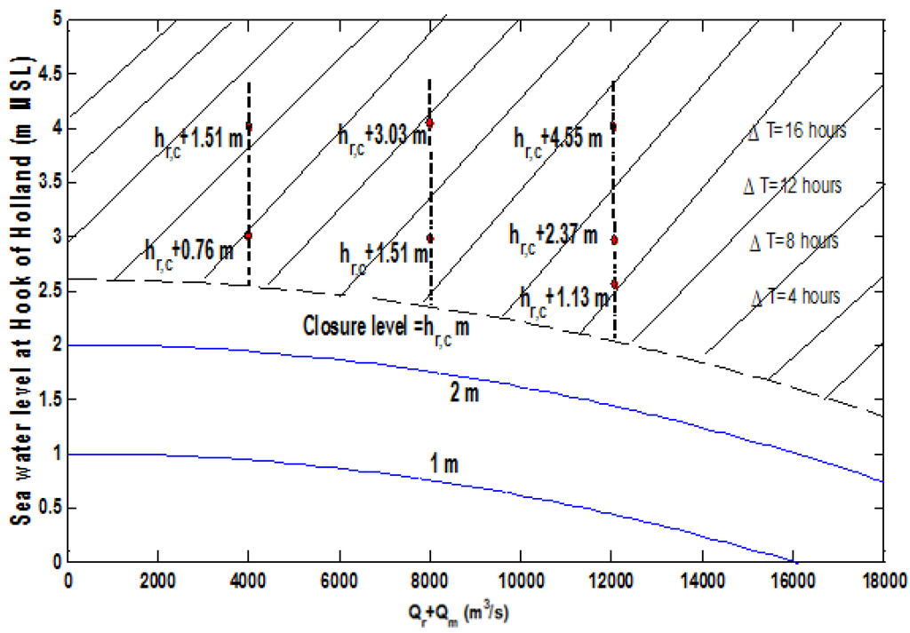
Figure A6.
Equal Level Curves with the closable delta at Rotterdam.
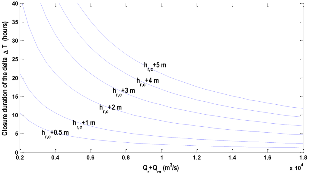
Figure A7.
Equal Level Curves with the closable delta at Rotterdam after the delta closes at hr,c.
Appendix B
Probability Distributions
The wind induced storm surge peak level hsmax fits the generalized Pareto distribution (GPD):
In this equation the shape parameter is −0.0677; the scale parameter is 0.3140 m; the location parameter u is 1.0 m.
The wind induced storm surge duration Ts fits the Weibull distribution
In this equation, Ts > 0, k is the shape parameter, 2.5237; is the scale parameter, 38.0887 hours.
The high Rhine discharge Qr fits the generalized Pareto distribution:
In this equation, is the shape parameter; is the scale parameter; u is the location parameter; and the parameters’ values are -0.0667, 1629.7 m3/s and 6000 m3/s respectively.
The high Meuse discharge Qm fits the Log-normal distribution:
In this equation, u is the mean value, 6.8667; is the stand deviation value, 0.3752.
The joint cumulative probability distribution of high Rhine flow and high Meuse flow fits a Gumbel Copula function:
where is estimated as 1.7158; Fr is the marginal distribution of high Rhine flow; Fm is the marginal distribution of the associated Meuse flow.
The joint probability distribution of storm surges and high Rhine flows
here I is an indicator function and hR is the highest Rotterdam water level calculated from the specific input variables using the 1-D model; 9/70 is the occurrence probability per year for the combination event of storm surges and high Rhine flows; hsmax stands for the wind induced storm surge peak, and its unit is m; Ts is the wind induced storm surge duration, and its unit is hours; hHW is the high tide level and hLW is the low tide level, their unit is m MSL; u is the time shift between peaks of tide and surge residual; Qr is Rhine discharge and Qm is Meuse discharge, their unit is m3/s; is the joint probability density distribution of Rhine discharge and Meuse discharge. More detailed information is in Zhong et al. [7].
References
- Mantz, P.A.; Wakeling, H.L. Forecasting flood levels for jointevents of rainfall and tidal surge flooding using extreme valuestatistics. Proc. Institut. Civil Eng. Res. Theor. 1979, 67, 31–50. [Google Scholar] [CrossRef]
- Acreman, M.C. Assessing the joint probability of fluvial and tidalfloods in the River Roding. J. Inst. Water Environ. Manage. 1994, 8, 490–496. [Google Scholar] [CrossRef]
- Gorji-Bandpy, M. The joint probability method of determining theflood return period of a tidally affected pond, Iran. J. Sci. Technol. 2001, 25, 599–610. [Google Scholar]
- Samuels, P.G.; Burt, N. A new joint probability appraisal offlood risk. Proc. Institut. Civil Eng. Water Maritime Eng. 2002, 154, 109–115. [Google Scholar] [CrossRef]
- Adib, A.; Vaghefi, M.; Labibzadeh, M.; Rezaeian, A.; Tagavifar, A.; Foladfar, H. Predicting extreme water surface elevation intidal river reaches by different joint probability methods. J. FoodAgric. Environ. 2010, 8, 988–991. [Google Scholar]
- Lian, J.J.; Xu, K.; Ma, C. Joint impact of rainfall and tidal level on flood risk in a coastal city with a complex river network: A case study for Fuzhou city, China. Hydrol. Earth Syst. Sci. Discuss. 2012, 9, 7475–7505. [Google Scholar] [CrossRef]
- Zhong, H.; van Overloop, P.J.; van Gelder, P. A joint probability approach using a 1-d hydrodynamic model for estimating high water level frequencies in the lower Rhine delta. Nat. Hazard. Earth Syst. Sci. 2013, 13, 1841–1852. [Google Scholar] [CrossRef]
- Bruno, M.; Annegret, H.T. Separating natural and epistemic uncertainty in flood frequency analysis. J. Hydrol. 2005, 309, 114–132. [Google Scholar]
- Efron, B. Bootstrap methods: Another look at the jackknife. Ann. Statist. 1979, 7, 1–26. [Google Scholar] [CrossRef]
- Efron, B.; Tibschirani, R.J. An Introduction to the Bootstrap; Chapman&Hall: New York, NY, USA, 1993. [Google Scholar]
- Davison, A.C.; Hinkley, D.V. Bootstrap Methods and Their Application; Cambridge University Press: Cambridge, UK, 1997. [Google Scholar]
- Dunn, P.K. Bootstrap confidence intervals for predicted rainfall quantiles. Int. J. Climatol. 2001, 21, 89–94. [Google Scholar] [CrossRef]
- Kysely, J. Coverage probability of bootstrap confidence intervals in heavy-tailed frequency models, with application to precipitation data. Theor. Appl. Climatol. 2010, 101, 345–361. [Google Scholar] [CrossRef]
- Roscoe, K.L.; Diermanse, F. Effect of surge uncertainty on probabilistically computed dune erosion. Coast. Eng. 2011, 58, 1023–1033. [Google Scholar] [CrossRef]
- Vrijling, J.K.; van Gelder, P.H.A.J.M. Probabilistic Design in Hydraulic Engineering; Delft University of Technology: Delft, The Netherlands, 1996. [Google Scholar]
- Zhong, H.; van Overloop, P.J.; van Gelder, P.; Rijcken, T. Influence of a storm surge barrier’s operation on the high water level frequency in the Rhine delta area. Water 2012, 4, 474–493. [Google Scholar] [CrossRef]
- van der Made, J. Design levels in the transition zone between the tidal reach and the river regime reach, hydrology of deltas. In Proceedings of the Bucharest Symosium, Bucharest, Rumania, 6–14 May 1969; pp. 246–257.
- Bol, R. Operation of the “Maeslant Barrier”: Storm surge barrier in the Rotterdam new waterway. In Flooding and Environmental Challenges for Venice and Its Lagoon: State of Knowledge; Cambridge University Press: Cambridge, UK, 2005; pp. 311–316. [Google Scholar]
- van Overloop, P.J. Operational Water Management of the Main Waters in the Netherlands; Delft Unversity of Technology: Delft, The Netherlands, 2009. [Google Scholar]
- van Overloop, P.J. Optimization of “Everything”, Prediction and Control of the entire Delta and River System of The Netherlands; Technical Report for Water INNovation (WINN); Delft University of Technology: Delft, The Netherlands, 2011. [Google Scholar]
- Dantzig, D.; Hemelrijk, J.; Kriens, J.; Lauwerier, H. Rapport Deltacommissie; Staatsdrukkerij En Uitgeverijbedrijf: 's-Gravenhage, The Netherlands, 1960. (In Dutch) [Google Scholar]
- Jorigny, M.; Diermanse, F.; Hassan, R.; van Gelder, P. Correlation analysis of water levels along dike-ring areas. Develop. Water Sci. 2002, 47, 1677–1684. [Google Scholar]
- Klerk, W.J.; Winsemius, H.C.; van Verseveld, W.J.; Bakker, A.M.R.; Diermanse, F.D. The co-incidence of storm surges and extreme discharges within the Rhine-Meuse Delta. Environ. Res. Lett. 2015, 10, 035005. [Google Scholar] [CrossRef]
- De Bruijn, K.M.; Klijn, F. Risky places in the netherlands: A first approximation for floods. J. Flood Risk Manag. 2009, 2, 58–67. [Google Scholar] [CrossRef]
- Ministerie van Verkeer en Waterstaat. Hydraulische Randvoorwaarden Primaire Waterkeringen, Voor de Derde Toetsronde 2006–2011 (hr 2006); Ministerie van Verkeer en Waterstaat: Den Haag, The Netherlands, 2007. (In Dutch) [Google Scholar]
© 2016 by the authors; licensee MDPI, Basel, Switzerland. This article is an open access article distributed under the terms and conditions of the Creative Commons by Attribution (CC-BY) license (http://creativecommons.org/licenses/by/4.0/).