Article

Semi- vs. Fully-Distributed Urban Stormwater Models: Model Set Up and Comparison with Two Real Case Studies

by
Rui Daniel Pina
1,2,*,
Susana Ochoa-Rodriguez
1,
Nuno Eduardo Simões
2,
Ana Mijic
1,
Alfeu Sá Marques
2 and
Čedo Maksimović
1
1
Department of Civil and Environmental Engineering, Imperial College London, London SW7 2AZ, UK
2
MARE—Marine and Environmental Sciences Centre, Department of Civil Engineering, University of Coimbra, Coimbra 3030-788, Portugal
*
Author to whom correspondence should be addressed.
Water 2016, 8(2), 58; https://doi.org/10.3390/w8020058
Submission received: 27 November 2015 / Accepted: 3 February 2016 / Published: 16 February 2016

Abstract

:
Urban stormwater models can be semi-distributed (SD) or fully distributed (FD). SD models are based on subcatchment units with various land use types, where rainfall is applied and runoff volumes are estimated and routed. FD models are based on the two dimensional (2D) discretization of the overland surface, which has a finer resolution with each grid-cell representing one land use type, where runoff volumes are estimated and directly routed by the 2D overland flow module. While SD models have been commonly applied in urban stormwater modeling, FD models are generally more detailed and theoretically more realistic. This paper presents a comparison between SD and FD models using two case studies in Coimbra (Portugal) and London (UK). To enable direct comparison between SD and FD setups, a model-building process is proposed and a novel sewer inlet representation is applied. SD and FD modeling results are compared against observed records in sewers and photographic records of flood events. The results suggest that FD models are more sensitive to surface storage parameters and require higher detail of the sewer network representation.

1. Introduction

Urban stormwater models are simulation tools that include algorithms and methods to describe the main physical processes related to the flow of stormwater across urban catchments. They are usually based on coupling three main modules: rainfall–runoff, overland flow and sewer flow. Rainfall is the main data input for the rainfall–runoff module that transforms it into the runoff. Runoff is then input to the overland module, which routes the flow over the urban surface area, and to the sewer flow module, which accounts for the flow in the sewer system.
Urban stormwater models can be considered semi-distributed (SD) or fully distributed (FD), depending on the spatial discretization of the rainfall–runoff module. SD models are based on subcatchment units with various land use types, where rainfall is applied and runoff volumes are estimated and routed. In FD models, runoff volumes are estimated and applied directly on the elements of a two-dimensional (2D) model of the overland surface. In SD models, conceptual empirical or physically based methods transform runoff routing into inflows hydrographs, which are applied to the selected computational nodes of the sewer system. Not every inlet is modeled but they are clustered to computational ones. FD models are based on a more realistic approach, since the generated grid-cell runoff is directly routed in the 2D overland flow module.
Traditional urban stormwater models have mostly been SD. One of the first widely implemented urban storm water models is the Storm Water Management Model (SWMM) [1] with an initial release in 1971. It is based on the integration of a rainfall–runoff and one-dimensional (1D) sewer flow modules, and was initially developed to analyze combined sewers overflows [2]. Later on, Ellis et al. (1982) [3] introduced the application of the overland flow module with the dual-drainage concept, by coupling a 1D sewer flow module with a 1D overland flow module that is known as 1D1D model. This concept was extended by Abbott (1993) [4] with a 2D model of the overland flow, which is known as 1D2D model.
However, the use of the overland flow module only had major developments with the introduction of the Geographical Information Systems (GIS) in the end of 1990s and first decade of 2000. At first, 1D1D models were significantly improved and opened the discussion about overland flow modeling [5,6,7,8,9]. In the late 2000s, 1D2D models become more popular with the development of technology and the increase in the computer power [10,11,12,13]. Nonetheless, rainfall–runoff modules that have been usually applied in urban stormwater modeling are commonly simplified with SD models. FD models have been typically applied in the large-scale hydrology modeling, with models like Mike SHE [14,15] and MOHID Land [16,17], amongst others. In these large-scale applications, modeled catchments usually have a larger area than the urban ones, coarser spatial resolution, and models do not take into account urban features, such as buildings and curbs.
Recent developments, however, bring new opportunities for detailed and physically based modeling of urban stormwater systems. Examples of important advancements are: increase of available data (e.g., digital map [18], advanced collaborative sources of information [19], weather radar data [20]); advances in technology (e.g., remote sensing [21], computing techniques [22]); and improvements of numerical methods (e.g., reduction in simulation times in 2D overland modeling [23], new mathematical approaches [24,25,26]). These improvements are opening the discussion for the application of FD urban stormwater models. Infoworks ICM [27] already implemented FD models, but its application has not yet become a standard practice in the water industry. Bailey and Margetts, 2008 [28] discussed the potential of FD models to replace the limitations of rainfall–runoff theories adopted in SD models. By analyzing a small case study, the authors achieved similar results with SD and FD models to demonstrate the viability of FD models, but they noted that FD models may still be computationally limited for large scale catchments and should require a significant amount of detailed information to represent all roof and gully connections. Chang et al., 2015 [29] compared different approach setups of 1D2D models applied to a mid-size real case study. They compared flood extents with performance indicators for different models, and concluded that a combination of SD and FD models is the suitable approach for the analyzed case study; however, they noted that FD models require information which is seldom readily available and pre-processing is therefore needed to generate/estimate such information (e.g., to define building connections).
This paper presents a full-scale comparison between SD and FD urban stormwater models and suggests innovative concepts for the model building process, and to establish the connection between modules of SD and FD models. The model building process proposed assigns the same data to both SD and FD models to enable a direct comparison of the two models. The connection between modules accounts for the limited sewer inlet capacity, and enable representation of the same interactions in both SD and FD models. The comparison of SD and FD models were based on two real case studies: Cranbrook catchment, London, UK; and Zona Central catchment, Coimbra, Portugal. The Cranbrook catchment has an area of 8.5 km2 and a flat topography, hence surface water ponding is the main cause of flooding. The Zona Central is a very steep catchment with an area of 1.5 km2 and the main cause of flooding is related with the insufficiency of inlet capacity, i.e., overland and gutter flow that cannot enter the sewer system. Comprehensive and detailed analyses of modeling results were applied for both case studies. In the Cranbrook catchment, modeling results were compared with flows and water depths records in sewers. In the Zona Central catchment, flooding extents have been analyzed based on photographic records of flooding events. Models were calibrated against monitoring data and photographic records of flooding events. Further analyses are presented with design rainfall events to access the importance of surface storage in both models.
The remainder of the paper is structured as follows: Section 2 presents insights into SD and FD modeling approaches and defines the concepts for model building and to represent the interactions between modules of SD and FD models. In Section 3, the case studies are introduced and Section 4 presents the comprehensive and detailed analysis of modeling results. Section 5 presents the discussion and conclusions of the presented work.

2. Semi- and Fully-Distributed Modeling Approaches

The concepts of SD and FD models are discussed in this Section, followed by the definition of the innovative model building process and the new sewer inlet representation proposed in this work. The model building process and sewer inlet concept were defined for the case studies implemented in Infoworks ICM v.5.5 software (Innovyze: Wallingford, UK) [27] and can be replicated for any urban stormwater modeling package.

2.1. Conceptual Basis of Semi-Distributed and Fully Distributed Models
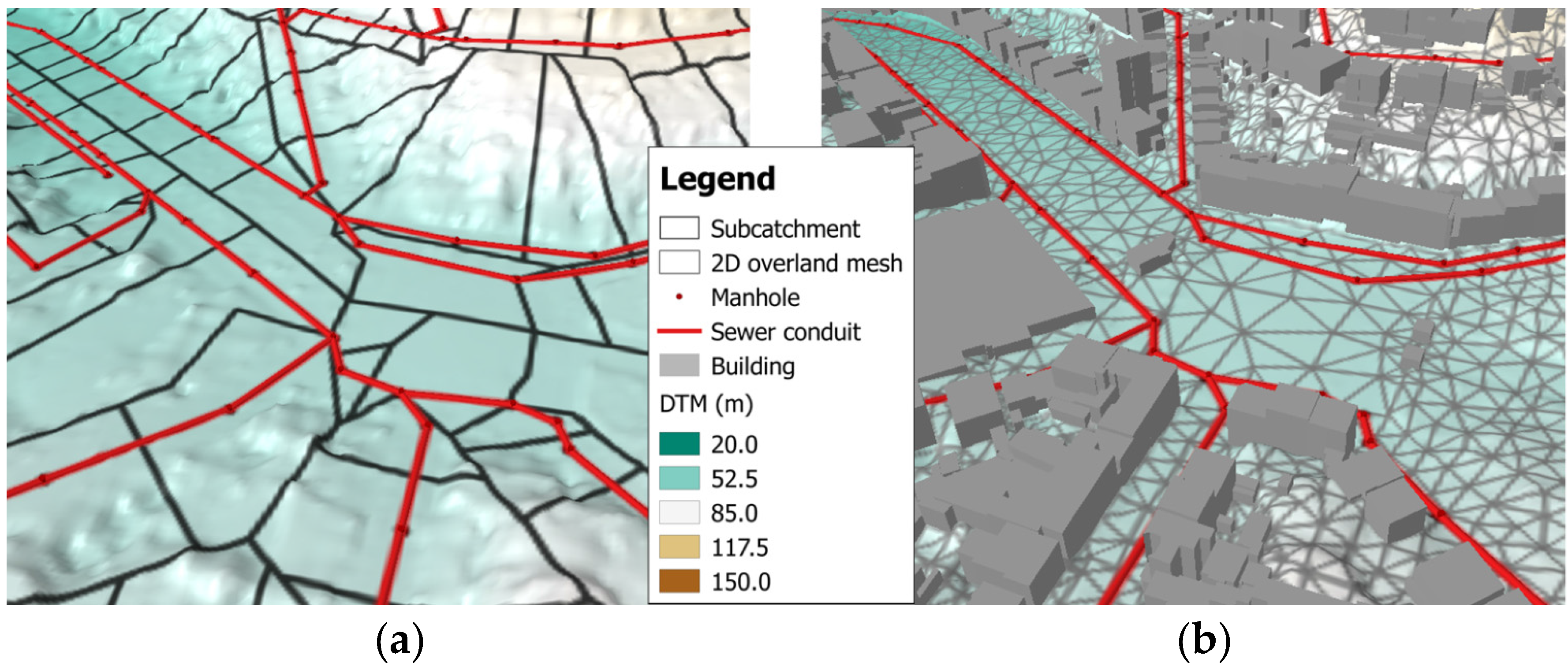
SD models are based on the definition of subcatchment units, delineated based upon analysis of the areas draining towards a given discharge point (Figure 1a). This discharge point is referred to as the subcatchment outlet, it is represented by a computational node and usually corresponds to a node of the sewer system. Each subcatchment unit is approximated by a regularly shaped surface to which uniform morphological and hydrological characteristics are assigned (e.g., area, mean slope, imperviousness, and infiltration properties). A spatially uniform rainfall input is assigned to each subcatchment. Runoff volumes are estimated for the subcatchment and are then routed to the subcatchment outlet by means of a conceptual or physically-based model. The result of this process are runoff hydrographs at the subcatchments’ outlets. SD models can be implemented in 1D, 1D1D and 1D2D models.
FD models are defined by a 2D overland mesh discretization (Figure 1b). The rainfall is directly applied to each 2D element, generating grid-point runoff, and the routing of surface runoff is then simulated directly by the 2D overland flow module. Therefore, FD models are physically-based that can replicate runoff processes more realistically. Moreover, because of the type of discretization, FD models can only be applied with 2D overland flow modules (1D2D models).
Figure 1. Semi-distributed (a) and fully-distributed (b) models.
Water 08 00058 g001
The main differences between SD and FD models are related to rainfall losses calculation (initial and continuing losses) and runoff routing. They can be summarized as follows.
  • Initial losses: The main difference is related to the representation of the depression storage. Depression storage is the stormwater that is retained in small depressions on the overland surface (puddle forming) and in pores of surface materials, both in impervious and pervious areas (surface wetting) [30]. In SD models, these two phenomena are usually considered with a constant value or a single value that is subtracted directly from the rainfall and is dependent on subcatchments’ slope and surface type [31]. In FD models, due to the finer resolution, the overland flow module can account for more detailed depressions that origin puddle forming [28].
  • Continuing losses: The main difference is related to the infiltration modeling. Infiltration is the percentage of rainfall draining into the soil. In SD models, infiltration is estimated for each subcatchment based on soil saturation, and subtracted from the rainfall before being applied to the model. In FD models, rainfall is applied directly to the overland mesh and infiltration is estimated for each 2D element, based on soil saturation and water depth. Therefore, infiltration predicted by FD models takes into account the runoff quantity on the overland surface, and can capture infiltration into permeable surfaces of runoff routed from upstream impermeable areas.
  • Runoff routing: In SD models, the generated runoff is transformed by the rainfall–runoff module into an inflow hydrograph that is usually applied to the sewer flow module. In FD models, the generated runoff is directly applied to the overland flow module and routed in the overland surface. SD runoff routing functions are based on both physically based as well as empirical or conceptual methods, with resolutions defined by subcatchments sizes [32,33]. FD runoff routing is simulated by applying physically based approaches with resolutions defined by the surface overland mesh. While FD models enable the representation of the real connection between impervious and pervious areas on the surface, SD models usually merge the runoff discharges to sewers from impervious and pervious area of subcatchments, unless the subcatchments are either pervious or impervious. In addition, runoff volumes captured by surface ponds are captured by FD models, since they consider the runoff on the overland mesh, whereas in SD models can neglect these volumes depending on subcatchment delineation and their discharge definition.

2.2. Model Building Process
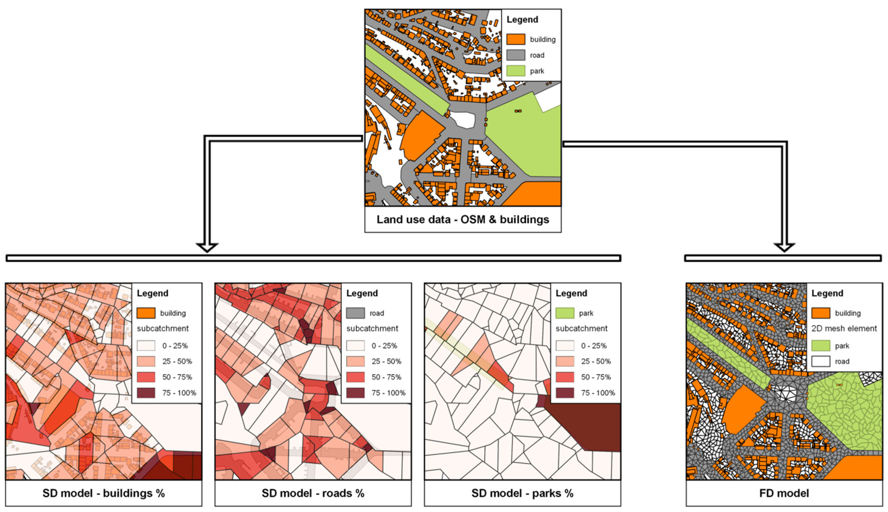
The proposed model building process was defined to assign exactly the same data to both SD and FD models. While the 1D sewer flow and the 2D overland flow modules are equally set up for both models (both SD and FD models can be based on the same 1D2D model), the rainfall–runoff module needs a different procedure to assign data to subcatchments in SD models, and to the overland surface mesh in FD models. The procedure proposed is based on assigning percentages of land use types for each subcatchment (in the SD model) and a land use category for each element of the overland surface mesh (in the FD model) (Figure 2).
In SD models, each subcatchment is defined by the percentage of the land use cover (e.g., has a percentage of area covered by road, parks, etc., each surface having the modeling attributes of the defined land use type). In FD models, each mesh element is characterized by one land use type (e.g., can be considered road or park with corresponding properties). The 2D mesh should be delineated considering boundaries of land use polygons to ensure that each 2D mesh element has only one land use type. Buildings polygons can be considered as voids in the 2D mesh, and their roof runoff is modeled in the FD model as subcatchments that discharge directly to the sewer network to take into account private connections. This procedure guarantees the input of the same data for both SD and FD models, despite their different spatial resolution.
Figure 2. SD (Semi-distributed) and FD (fully distributed) rainfall–runoff land use assignment.
Water 08 00058 g002

2.3. Connections between Modules and Inlet Capacity
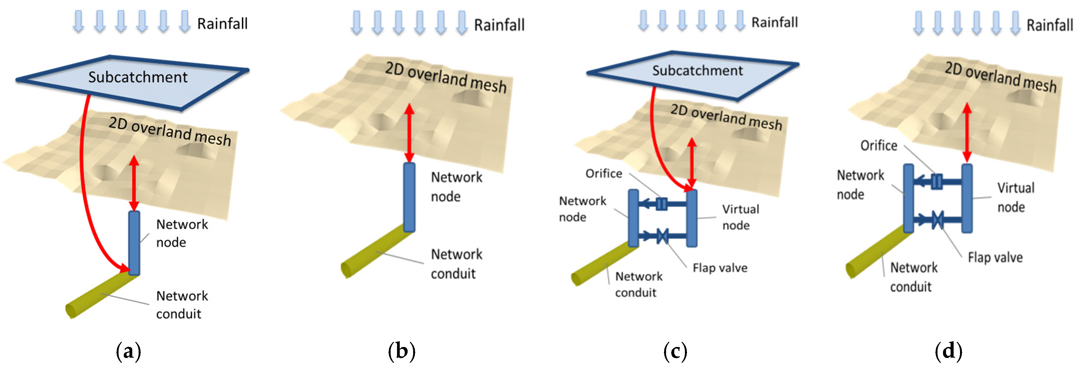
The amount of water entering the sewer system is, in reality, limited by the capacity of sewer inlets; nonetheless, this fact is not always considered in urban drainage models. SD models can take into account the inlet capacity if the subcatchments are delineated for each sewer inlet. However, SD models usually apply all the runoff estimated in a given subcatchment directly into the selected computational node of the sewer system, without accounting for the inlet capacity (Figure 3a). Neglecting the limited capacity of inlets means that the model fails to represent the stormwater ponding and flooding that may occur due to limited inlet capacity, even before runoff reaches the sewer system. As a result, flooding only occurs when the sewer system surcharges.
FD modeling packages, such as Infoworks ICM v.5.5 software [27], have included the inlet capacity of sewer inlets in network nodes connected with the 2D overland surface mesh (Figure 3b). In general, a weir or orifice equation is defined in the manhole to control the inlet capacity with the water level on the surface.
To overcome the limited representation of sewer inlets in SD models, a concept based on virtual nodes was developed, as represented in Figure 3c. These virtual nodes have an infinitesimal volume, and are directly connected with the overland surface and with subcatchments. They are also connected with the sewer network manholes through orifices with the limited capacity of sewer inlets. Therefore, the inflow to the sewer system from subcatchments discharges and overland module is limited by the inlet capacity of gullies defined by the discharge curve of orifices. If the inlet capacity is exceeded, runoff remains on the overland surface, as it cannot enter the sewer systems. In addition, flap valves were adopted in the opposite direction of orifices to enable runoff to flow from the sewers onto the 2D surface model once sewer surcharge occurs. The discharge curve that defines sewer inlets capacity is based on recommendations presented by Pina et al. (2010) [34] and Ally (2011) [35].
To consider the same inlet capacity in SD and FD models, the representation of sewer inlets in FD models was based on an equivalent concept as defined for SD models but without subcatchments (Figure 3d). The sewer inlet concept typically defined in FD models (Figure 3b) was not adopted to guarantee the same connections between modules in both SD and FD models, making them comparable.
Figure 3. Connections of rainfall–runoff with overland and sewer flow modules: (a) traditional connections for SD models; (b) traditional connections for FD models; (c) developed connections for SD models; and (d) developed connections for FD models.
Water 08 00058 g003

3. Case Studies

The selected case studies are the Cranbrook catchment, in London, UK, and the Zona Central catchments, in Coimbra, Portugal. For each case study, SD and FD models were implemented in Infoworks ICM v. 5.5 [27] based on the same 1D sewer network and 2D overland flow models (1D2D models). To enable comparison between both case studies, similar data were collected to build the models. The sewer flow model was built with the network and operational data, provided by the respective water companies of the study catchments. The 2D overland flow model was created based on available LiDAR-based Digital Terrain Models (DTM) with 1 m horizontal resolution. Buildings polygons and land use data were used to characterize the model (e.g., roughness and infiltration parameters) and to define the surface mesh (e.g., mesh resolution, break lines, voids, and boundaries). The land use data were obtained from the OpenStreetMap [19] and buildings polygons were provided by local authorities. The SD models for these case studies have been developed and updated since 2010 and 2009, respectively [34,36]. These SD models were improved and calibrated following the UK standards [37] using local rainfall and flow records. The FD model for both case studies was developed with the exact same data as the calibrated SD model, following the methodology presented in Section 2, so as to achieve comparable models.

3.1. Cranbrook Case Study

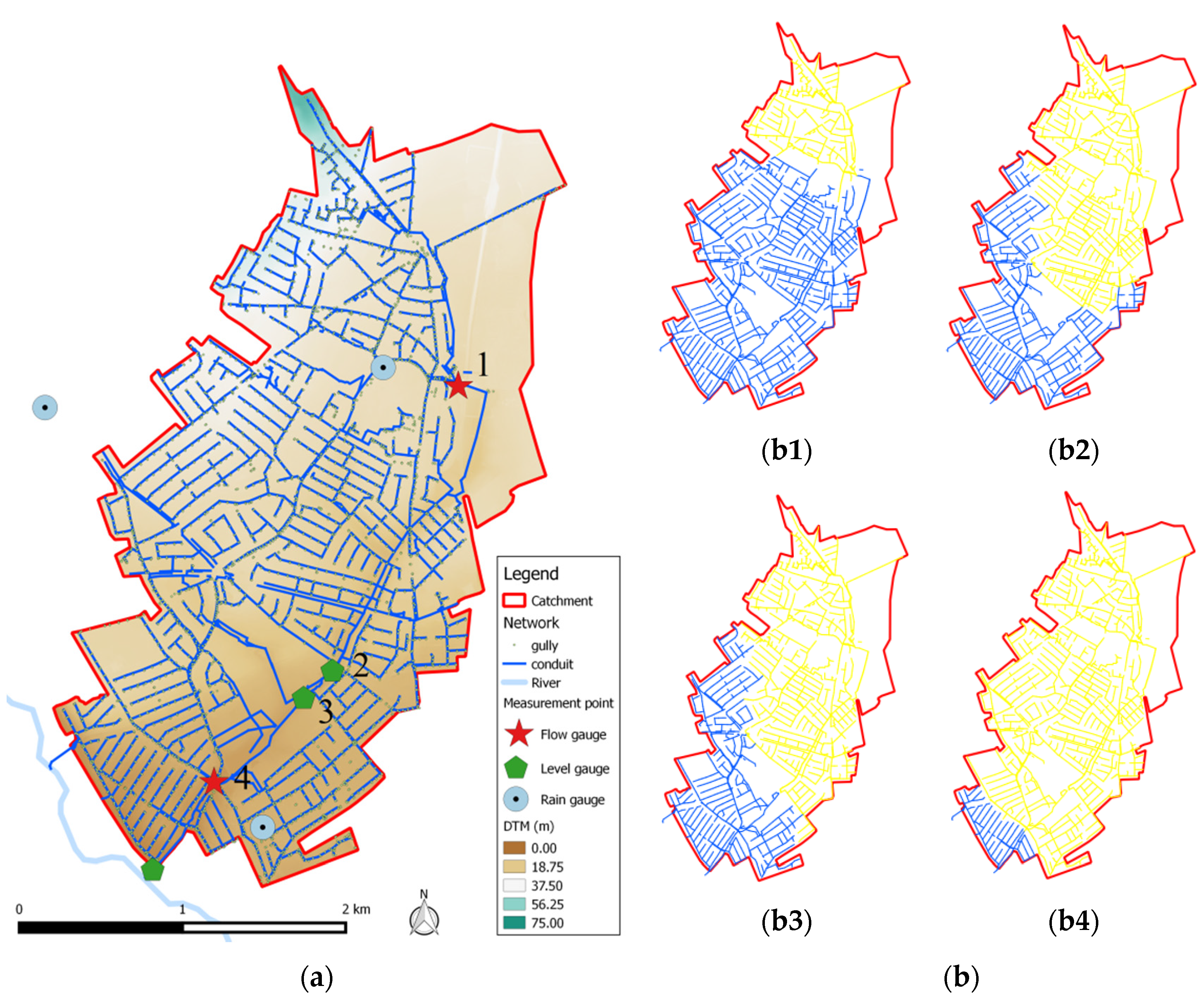
The Cranbrook catchment is located in the North-East part of London, UK, and is presented in Figure 4. It is predominantly urban (residential and commercial units), with some open green spaces. It covers an area of 8.5 km2 with an average slope of 5%. The stormwater sewer system is nearly 98 km long; it is mainly separate and discharges into the Roding River. This catchment has suffered several floods during recent years (e.g., in 2000 and 2009), which have affected hundreds of properties.
A real time monitoring system has been operated in the Cranbrook catchment since April 2010 (Figure 4b). It includes four rain gauges, three water level sensors (one in sewers and two in channels) and two flow gauges in sewers that record water depth and velocity. The most upstream sensor (Barkingside) was installed in December 2014, and covers a limited area of 2 km2 that is mostly residential. Valentine sewer and Valentine channel sensors are located almost in the middle of the catchment, with upstream drainage areas of 5.0 and 5.5 km2, respectively. As the names suggest, one sensor is installed in the sewers entering Valentine Park and the other on an open channel in the Park. Cranbrook sewer is a sensor installed in the downstream area and covers most of the catchment area (8.0 km2). There is also a level gauge in the main discharge of the catchment to validate the outfall conditions, since they can be influenced by the level of Roding River.
Figure 4. Cranbrook case study—London, United Kingdom: (a) DTM (Digital Terrain Model) and network data. (b) Monitoring stations and upstream network: (b1) Barkingside (flow and depth sensor); (b2) Valentine sewer (depth sensor); (b3) Valentine channel (depth sensor); and (b4) Cranbrook sewer (flow and depth sensor).
Water 08 00058 g004
The SD and FD models for the Cranbrook case study include a 1D network based on a sewer system with 2596 conduits and 2546 manhole nodes. The conduits have an average slope of 1% and cross sections with diameters ranging from 100 mm to 1950 mm. The 1D network also includes 565 m of open channels with cross sections of up to 6 m width, and five storage ponds, four of which are recreational lakes. The SD rainfall–runoff model has 4409 subcatchments with areas ranging from 50 m2 to 40 ha, and average of 0.2 ha; slopes are varying from 0.015 m/m to 0.408 m/m with an average of 0.05 m/m, and widths are ranging from 4 m to 357 m, with an average of 22 m. It considers initial losses dependent on subcatchments’ slopes and the Wallingford routing model. Infiltration losses are estimated for both SD and FD models with fixed runoff coefficients. The overland flow module, which defines the resolution of the FD model, is based on a 2D mesh with 117,712 elements with areas ranging from 25 m2 to 992 m2 and mean of 61 m2.

3.2. Zona Central Case Study

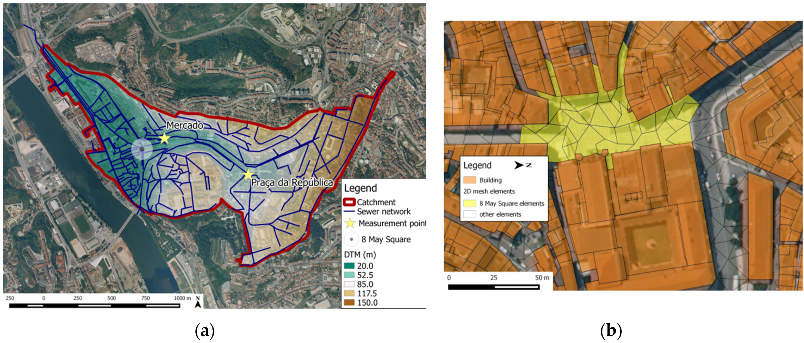
The Zona Central catchment is located in Coimbra, Portugal (Figure 5). It covers highly urbanized zones, mainly residential and commercial, including the downtown area of Coimbra, where important services and historical buildings are located. It has a total drainage area of approximately 1.5 km2 with an average slope of 24%. The sewer system is nearly 35 km long, most of which is combined and discharges into the Coselhas brook and into the Coimbra Waste Water Treatment Plant, from where it is further directed to Mondego River. This catchment has suffered several floods during recent years, the occurrence of which is exacerbated by the steep topography and the limited inlet capacity of the sewer system. The area at highest risk of flooding is the Praça 8 de Maio (Figure 5b), a square in the center of the catchment, where important services are located (e.g., City Council and tourist attractions) and where flood waters tend to pond due to topographic conditions.
Figure 5. Zona Central catchment—Coimbra, Portugal: (a) sewer network, DTM and monitoring point locations; and (b) extents of Praça 8 de Maio.
Water 08 00058 g005
A monitoring campaign was conducted in this catchment between 2010 and 2012 by Simões, 2012 [36]. The campaign included three rain gauges and two water depth sensors. The latter were located along the main sewer, upstream of the Praça 8 de Maio, covering drainage areas of 0.4 km2 in the “Mercado” station and 1.0 km2 in the “Praça da Républica” gauges (Figure 5a), respectively. In addition, the water utility of the area—AC, Águas de Coimbra E.M.—has maintained a single rain gauge in the catchment for several years (since approximately 2005); from this gauge continuous rainfall records are available, including records of flood-generating storms. The data collected between 2010 and 2012 were used to calibrate the SD model and the rain gauge records collected by Águas de Coimbra are used as input for the flood simulations presented in this paper.
The SD and FD models for the Zona Central case study are based on a 1D sewer network model comprising 1016 conduits and 1014 manhole nodes. The conduits have an average slope of 5% and cross-sections with dimensions ranging from 200 mm circular diameter to closed rectangular section of dimensions 3.5 × 1.7 m2. The SD rainfall–runoff model has 911 subcatchments with areas ranging from 50 m2 to 4.8 ha and a mean of 1722m2, slopes ranging from 0.00 m/m to 1.13 m/m and a mean of 0.24 m/m, and widths ranging from 6 m to 493 m and a mean of 51 m. In the SD model, initial losses are given as an absolute value and runoff volumes are routed to subcatchments’ outlets using the SWMM routing model. For both SD and FD models, infiltration losses are estimated with the Horton equation for pervious areas, whereas a fixed runoff coefficients approach was adopted for impervious areas. The overland flow module, which defines the resolution of the FD model, is based on a 2D mesh with 10,741 elements, with areas ranging from 25 m2 to 678 m2, with a mean of 89 m2.

4. Results and Discussion

4.1. Cranbrook Case Study

The analysis of the Cranbrook case study was based on three selected events, for which rainfall and water depth and flow records in sewers were available. The rainfall records are summarized in Table 1, considering the average rainfall in the entire catchment area. For each event, the entire day was simulated, but only the time frame corresponding to the main rainfall event was analyzed to minimize errors related to the impact of the initial conditions.
Table 1. Summary of rainfall records used for the Cranbrook case study.
Event ID *StartEndDuration (h)Maximum Rainfall (mm/h)Total Rainfall Depth (mm)Average Rainfall Intensity (mm/h)
14121212 December 2014 1:30 A.M.12 December 2014 8:00 A.M.6.51210.92
1501033 January 2015 3:50 A.M.3 January 2015 5:00 P.M.13.21216.61
1501088 January 2015 7:30 A.M.8 January 2015 2:30 P.M.7.01211.62
Note: * This code represents yymmdd and it is used in the next figures to reference these events.
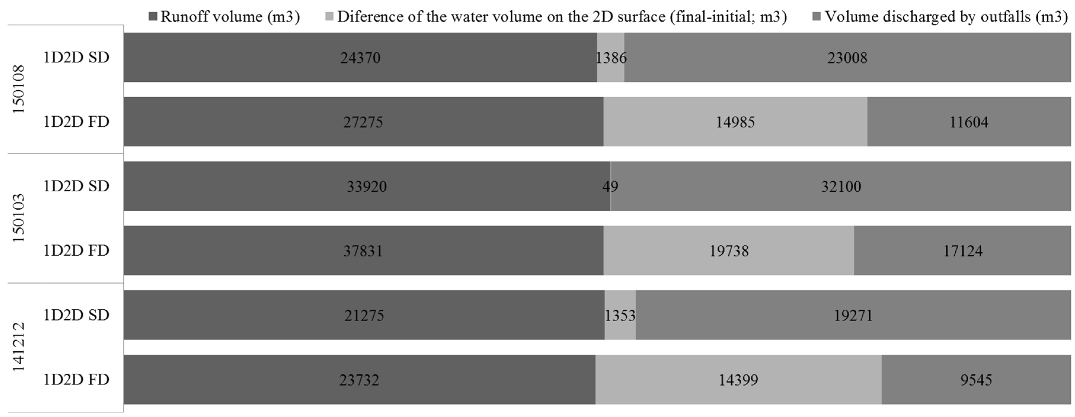
The balances presented in Figure 6 show the distribution of volumes among the modules for all the events analyzed. Runoff volumes were generated by the rainfall–runoff module, and they were calculated with the subcatchments discharges in SD models, and with the runoff volume generated on the 2D mesh in FD models. Volumes in the overland flow module were calculated with the difference between volumes at the end of the simulation with the ones at the beginning of each event. The volumes in the sewer flow system were defined by the discharges at outfalls in the 1D sewer network.
In all three events, total runoff volumes are similar to the total combined volumes from overland and sewer flow modules. The insignificant differences in the total runoff volumes are caused by small differences in subcatchments’ areas in the SD model when compared to the FD model. However, in all simulations FD model retained more water on the surface in contrast to SD model, where most of the runoff is conveyed through the drainage system.
Figure 6. Volume balance for the Cranbrook case study model runs.
Water 08 00058 g006
To further explore the source of water accumulation on the overland surface, the differences between FD and SD maximum volumes at the surface were divided by land use groups (Figure 7). The most significant differences are observed for roads and buildings (residential, retail and industrial areas) zones, leading to the conclusion that runoff on the overland in FD models is retained due to surface ponding and building singularities. The category “Other areas” includes non-classified zones in the land use data that cover a mix between open areas and zones covered by buildings.
Figure 7. Differences between runoff volumes on the overland surface generated by SD and FD models, distributed by land use groups in Cranbrook case study. The bars correspond to the three storm events under consideration (see Table 1).
Water 08 00058 g007
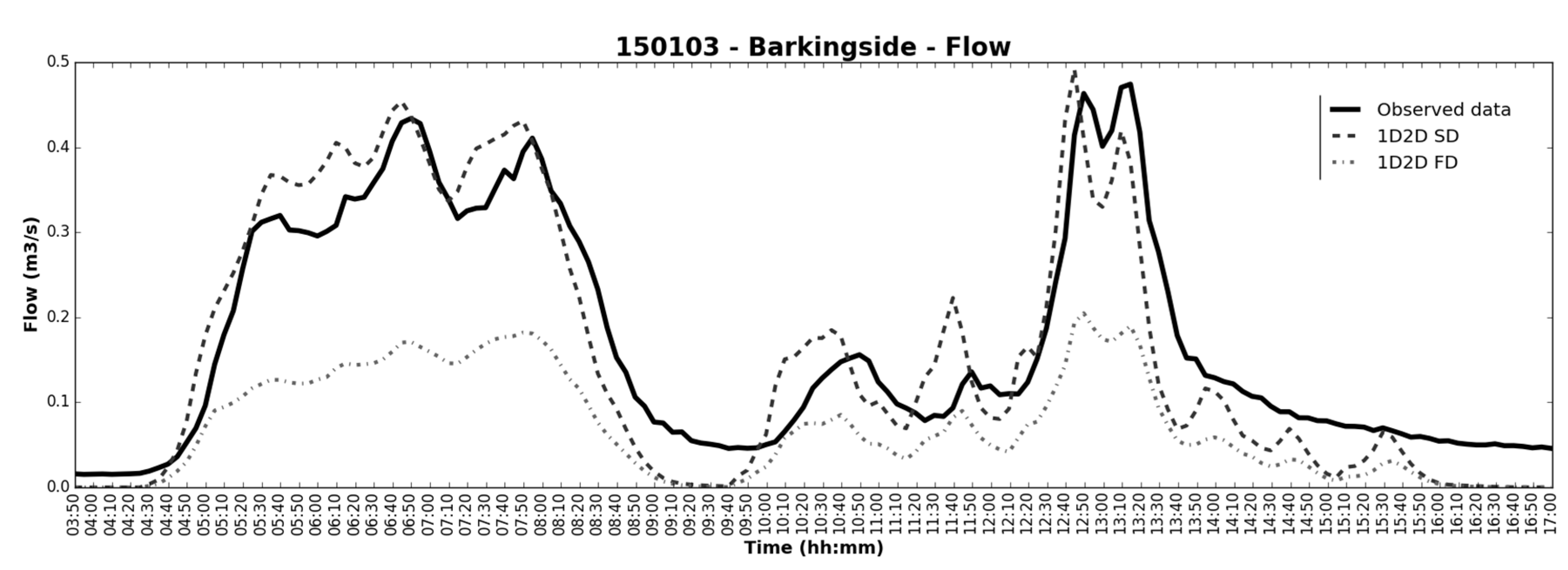
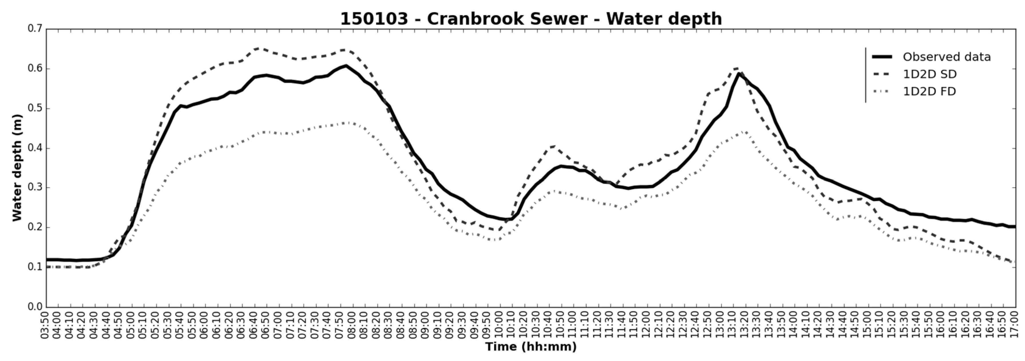
As water volumes in the sewer flow module are generally lower in FD than in SD models, FD results tend to underestimate water depth and flows in sewers, as exemplified in Figure 8 and Figure 9 with two monitoring locations for Event 150103. These figures also show the correct calibration of initial losses (intersection and depression storage) in both models, because flow is initialized at the same time as observed data. In general, SD results tend to predict temporal pattern and peak values with more accuracy.
Figure 8. Predicted flow and observed data in the Barkingside gauge for Event 150103—Cranbrook case study.
Water 08 00058 g008
Figure 9. Predicted water depth and observed data in the Cranbrook Sewer gauge for the Event 150103—Cranbrook case study.
Water 08 00058 g009
The last considerations are generalized to all the events simulated with the statistical analysis presented in Figure 10, based on the following indicators:
  • Relative error (RE) in peak (Figure 10, left column):
    RE = ( Vmax obs Vmax res ) / Vmax obs
    where RE is the relative error in the peak results ( Vmax res ) compared to the peak in observed data ( Vmax obs ). RE was applied to flow and water depth peaks. Positive RE values indicate underestimation by the peak results and negative values imply overestimation. The RE has the advantage of being a “tangible” statistic that evaluates the performance of a critical parameter such as the peak flow or water depth. It is important to note that very large RE can be obtained when low values are evaluated, even if the absolute difference in peak is small.
    In general, for all simulated events the RE is higher in FD than in SD models, which means that FD underestimates results against observed data. In the Cranbrook sewer sensor, the SD model predicted accurate water depths but overestimated flows. This can be due to the location of the sensor in a zone where turbulence can occur and affect monitoring data accuracy. In the FD model this variation does not occur, because both water depth and flows results are smoothened and underestimated. In conclusion, while the SD model captured water depth and flow peaks, the FD model underestimated these results.
  • Coefficient of determination (R2) (Figure 10, middle column) and Regression coefficient (β) (Figure 10, right column): Resulting from a simple linear regression analysis applied between each simulated results time series and the observed data. These two statistics provide an indication of how well the results replicate observed data, both in terms of pattern (R2) and accuracy (β). The R2 measure ranges from 0 to 1 and describes how much of the observed data variability is according with the simulated results. In practical terms, R2 provides a measurement of the similarity between the patterns of the observed data time series and the simulated results time series, i.e., indicates how the hydrodynamics are captured by the model. The regression coefficient, β, is employed to provide supplementary information to the R2. β 1 represents good agreement in the magnitude of observed data and results time series; β > 1 means the results are overestimated against observed data (by a factor of β); and β < 1 means the results are underestimated against observed data (by a factor of β).
    For most simulated events, the R2 is close to 1 for both SD and FD models, which implies that the variations of modeling results match the observed data, i.e., the models can capture the hydrodynamics of observed data. The differences between SD and FD models are not so evident, but FD models tend to have higher R2, which suggest that they have the potential to better represent the dynamic behavior of stormwater flows in urban catchments.
    The β is in general closer to 1 for SD model results, which indicates that SD results are matching the observed data more accurately than FD ones. The exceptions in the results analysis can be noticed in the data for the Valentines and the Cranbrook Sewer sensors. For the Valentines Sewer sensor, network elements tend to overestimate water depths in the SD model. For the Cranbrook Sewer sensor, the errors in observed flow data due to turbulence also affect this indicator as verified for the RE. These two aspects are not verified in the FD model as it underestimates overall results.
    Combining the R2 and the β results, it can be concluded that SD and FD models capture the hydrodynamics registered and the SD model tend to capture the magnitude of observed data while FD model underestimates it.
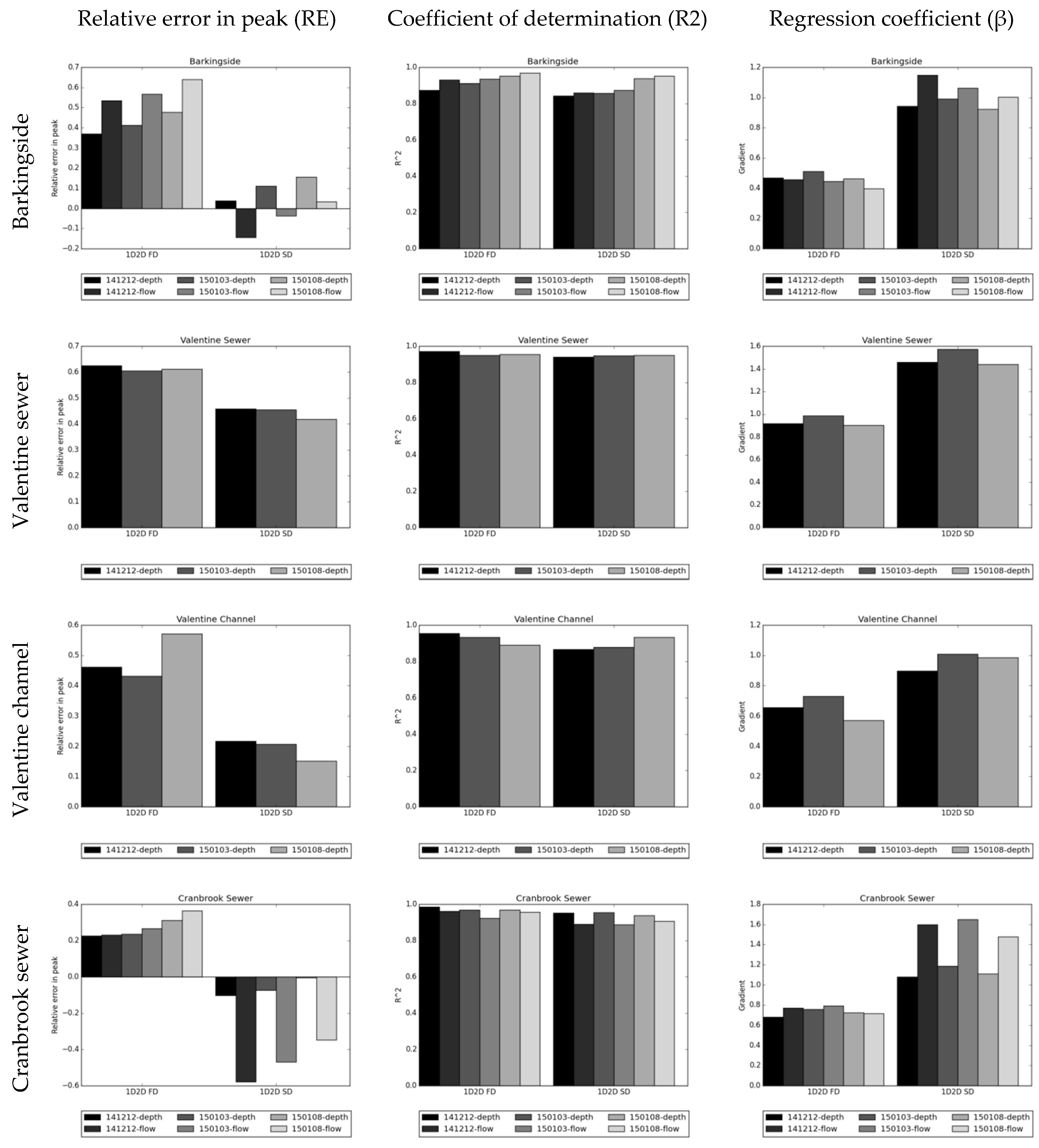
Figure 10. Statistical analysis of modeling results against observed data of Cranbrook case study.
Water 08 00058 g010

4.2. Zona Central Case Study

The analysis of the Zona Central case study was based on four flooding events for which rainfall records and photographic records of the flooding in Praça 8 de Maio were available. The rainfall records are summarized in Table 2, considering the average rainfall in the entire catchment area.
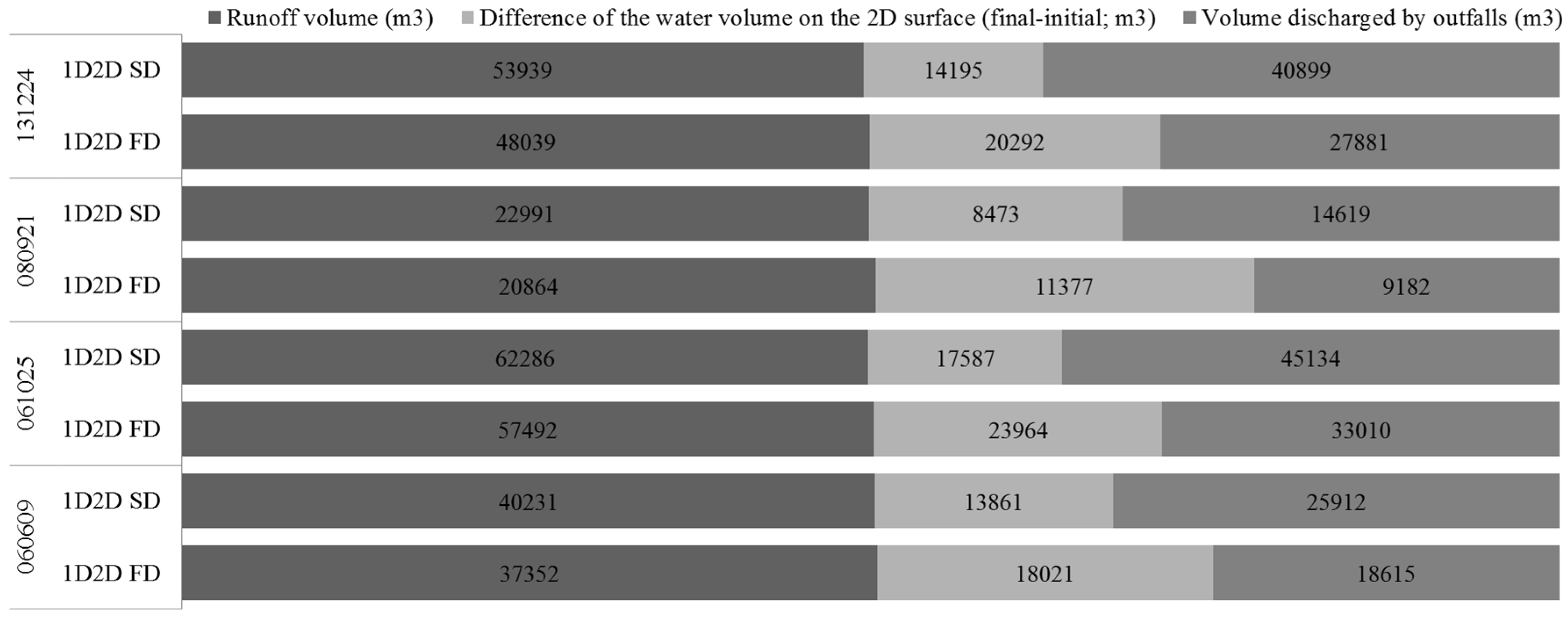
The balances presented in Figure 11 show the distribution of volumes between the modules for all the events analyzed, in accordance to the analysis presented before for the Cranbrook case study. In this case study, FD models also tend to have higher water volumes at the 2D overland surface than in SD models, and less volume discharged by the outfalls of the 1D sewer network. However, in this case study the differences between SD and FD models are not as significant as for the Cranbrook catchment. This is because the rainfall events selected caused floods in both SD and FD models, which increased the overland surface volumes in the SD model. There are also insignificant differences in the runoff volumes caused by small differences in buildings’ area at the boundary of the catchment in the FD model.
Table 2. Summary of rainfall records in Zona Central case study.
Event Name *StartEndDuration (h)Maximum Rainfall (mm/h)Total Rainfall Depth (mm)Average Rainfall Intensity (mm/h)Return Period (yr.)
0606099 June 2006 2:50 P.M.9 June 2006 4:30 P.M.1.7144.036.622.050
06102525 October 2006 12:30 A.M.25 October 2006 5:30 A.M.5.0102.056.611.350
08092121 September 2008 3:10 P.M.21 September 2008 5:20 P.M.2.260.621.49.95
13122424 December 2013 6:40 A.M.24 December 2013 6:00 P.M.11.331.548.94.35
Note: * This code represents yymmdd and it is used in next figures to reference these events.
Figure 11. Volumes balance for the Zona Central case study model runs.
Water 08 00058 g011
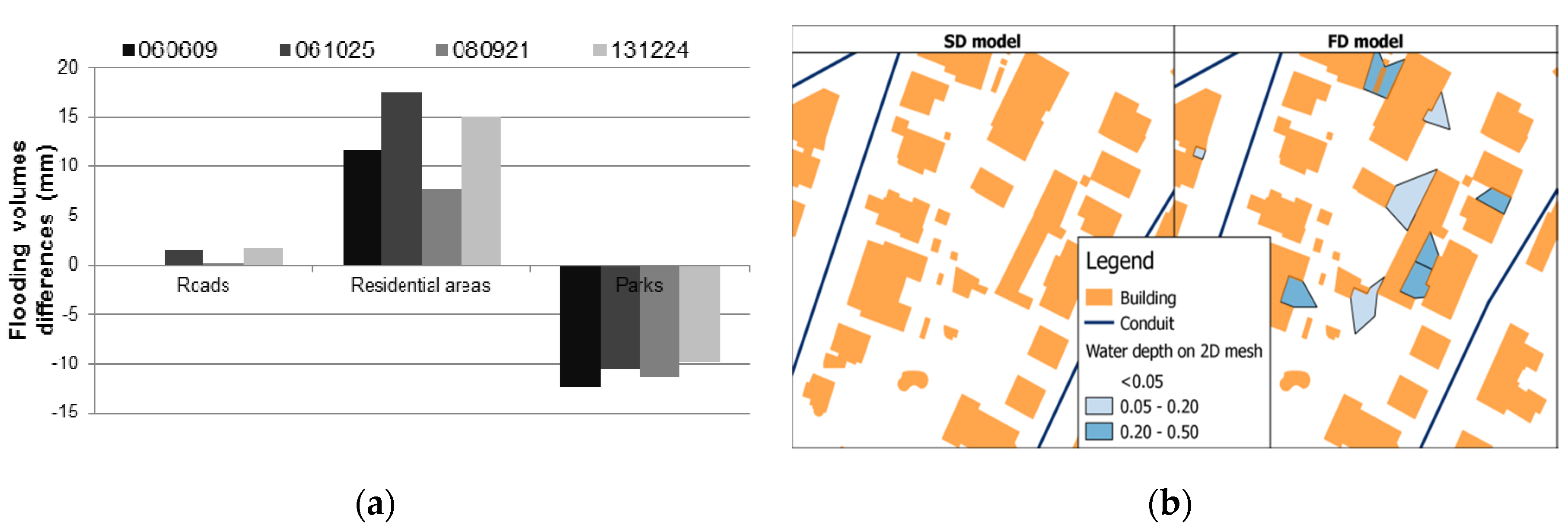
To investigate where the FD model retains water on the surface, Figure 12a presents the differences between FD and SD maximum volumes on the surface divided by the land use groups. Larger discrepancies are registered in zones covered by buildings (residential areas). This means that runoff is retained on the overland surface in FD models due to building singularities, as exemplified with Figure 12b, and surface ponding on roads is not a significant problem, opposite to the Cranbrook case study.
Figure 12. Differences in runoff volumes on the overland surface generated by SD and FD models in Zona Central case study: (a) runoff volumes distributed by land use types; and (b) example of runoff retained on the overland surface in FD models due to building singularities.
Water 08 00058 g012
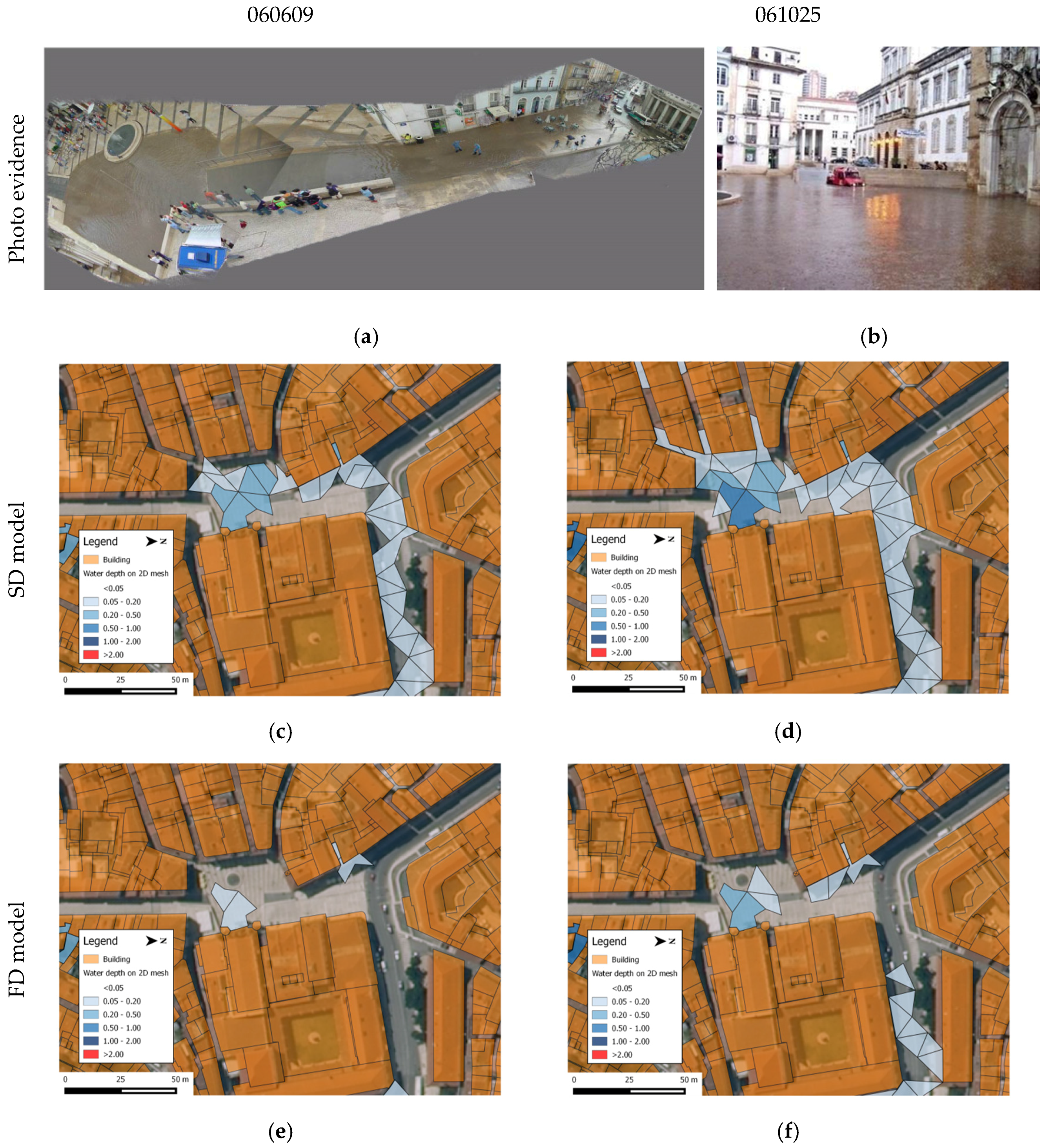
The comparison of floodplains generated in the Praça 8 de Maio is summarized in Table 3 for all the events analyzed. In general, flooding volumes are higher in SD than in FD model, and water depth and flooding areas follow the same pattern. This means that as FD model stores more water on the overland surface, runoff volumes are retained in the upstream areas and do not get to lower zones where water accumulates in reality. The predicted floods at Praça 8 de Maio were also compared to photographic records of floodplains, as presented in Figure 13 for the events with the two highest return periods. It can be concluded that flooding extent is well predicted with the SD model, but underestimated with the FD model.
Figure 13. Comparison of photograph records with predicted floodplains on Praça 8 de Maio, Zona Central case study. (a) Flood registered on Event 060609, photo adapted from [38]; (b) Flood registered on Event 061025, photo courtesy of local newspaper Diário de Coimbra; (c) Floodplain generated by the SD model for Event 060609; (d) Floodplain generated by the SD model for Event 061025; (e) Floodplain generated by the SD model for Event 060609; (f) Floodplain generated by the FD model for Event 061025.
Water 08 00058 g013
Table 3. Summary of modeling results on Praça 8 de Maio, Zona Central case study.
EventMax Water Depth (m)Flooding Volume (m3)Flooding Area (m2)
SDFDSDFDSDFD
0606090.440.11275681092324
0610250.510.253601381693630
0809210.100.086342324248
1312240.140.067934569248

4.3. Assessing the Importance of Surface Storage as a Function of Rainfall Magnitude

The aforementioned analyses indicate that, in general, FD models retain larger volumes of water on the overland surface as compared to the corresponding SD setup. Depending on the case study, the volume retained can be stored in surface depressions, as occurred in the Cranbrook case study, or it can be retained in building singularities, as occurred in the Zona Central case study. To analyze the importance of the surface storage in relation to the rainfall intensity, an analysis based on design storms was performed. The models of Cranbrook case study were tested with five design storms with returns period (RP) of 10, 20, 30, 100 and 200 years, and the models of Zona Central case study were tested with six design storms with RP of 2, 5, 10, 20, 50 and 100 years.
Figure 14 and Figure 15 present the relative flooding volumes for each land use group type, calculated based on the maximum water depth predicted at the 2D mesh of the overland surface. It can be concluded that the percentage of flooding volume on roads is higher in the SD model for the two case studies. In both situations, the increase of the rainfall return period, and thus intensity, led to decrease of the relative volumes in roads and an increase of volumes in areas covered by buildings for both SD and FD models.
Figure 14. Relative flooding volumes on each land use group for design storms events, Cranbrook case study.
Water 08 00058 g014
Figure 15. Relative flooding volumes of each land use group for design storms events, Zona Central case study.
Water 08 00058 g015
Figure 16 shows the difference between SD and FD models in predicting flooding volumes for each land use group type in the Cranbrook case study. In addition to the increase in the relative volume in residential areas, as shown in Figure 14, the differences in flooding volumes between SD and FD models are similar in residential areas for all events. For roads, the flooding volume decreases as water tends to accumulate more in these zones leading to higher volumes in the SD model for high rainfall intensities. Figure 17 presents the same analysis applied to the Zona Central case study. In this catchment, the increase in the rainfall return period led to the increase in the difference between FD and SD volumes for both roads and residential areas. This means that with the increase in the rainfall intensity, higher volumes are retained on the overland surface by the FD model, as compared to the SD simulations.
Figure 16. Differences on flooding volumes of each land use group for design storms events, Cranbrook case study.
Water 08 00058 g016
Figure 17. Differences on flooding volumes of each land use group for design storms events, Zona Central case study.
Water 08 00058 g017
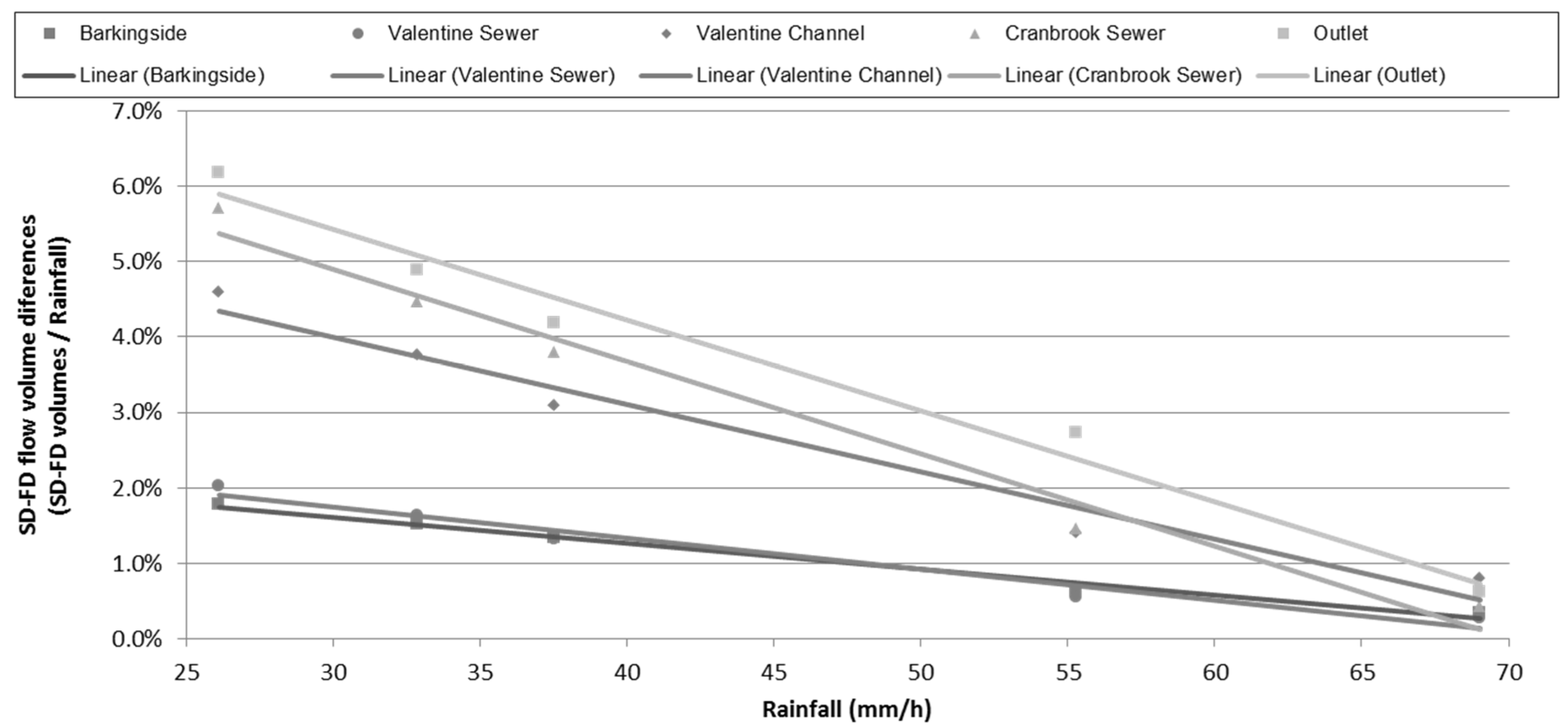
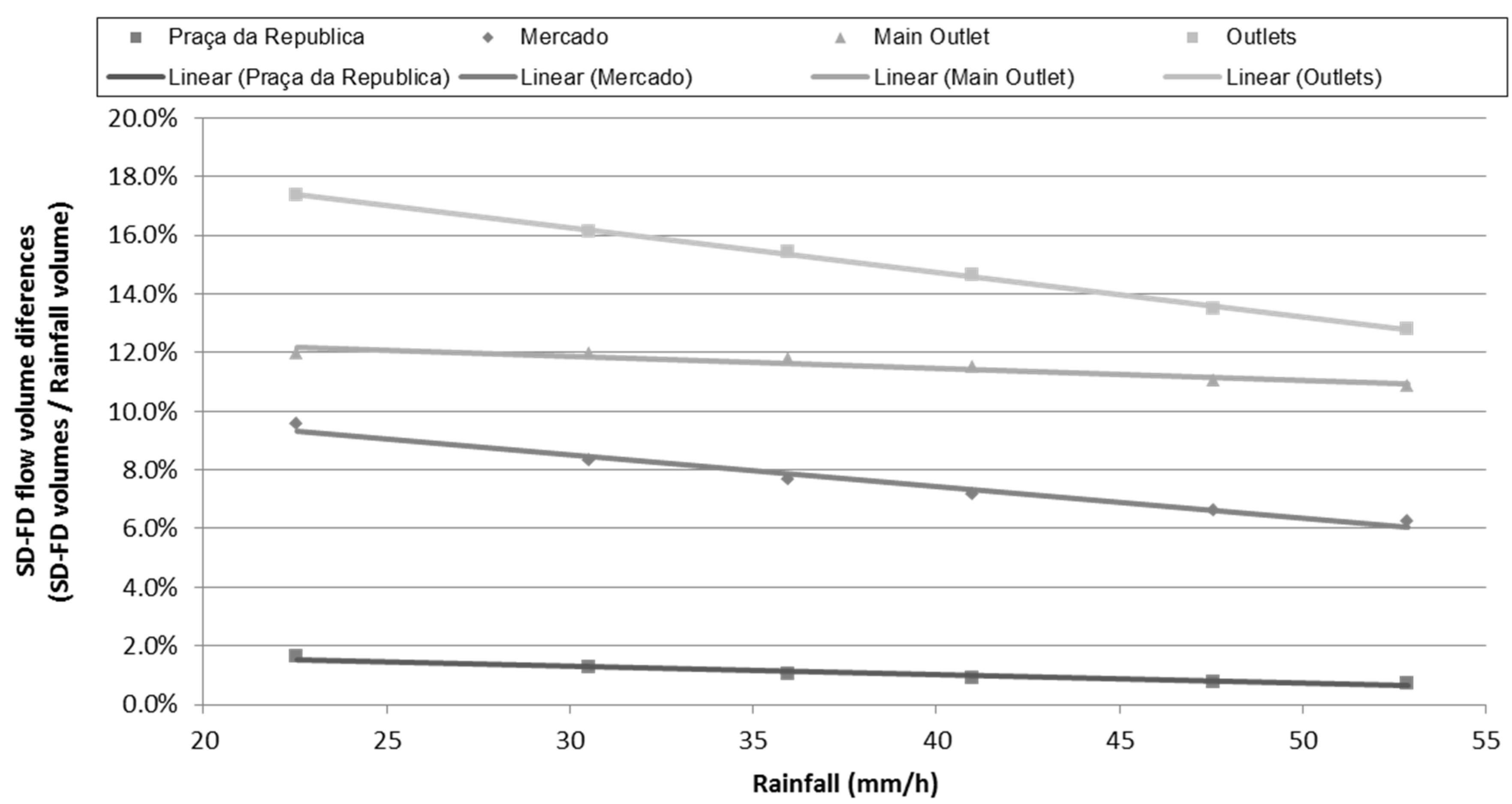
To assess the importance of the volume that is retained on the overland surface, Figure 18 and Figure 19 analyze the differences between flow volumes in the 1D network. It can be verified that differences between SD and FD models rise with the increase in drainage areas and decrease for higher intensity rainfalls. However, the differences have significantly distinct trends for each case study. In the Cranbrook case study, surface storage can be neglected for high intensity rainfalls, converging to low percentages for all monitoring point locations. In the Zona Central case study, however, surface storage is significant for downstream monitoring point locations for all the rainfall intensities tested. While in Cranbrook case study the surface storage is mainly related with surface depressions, in the Zona Central catchment the surface storage verified in the FD model is also related to buildings singularities, and the absence of data about private drainage networks and connections.
Figure 18. Differences on flow volumes in the 1D network for design storms events, Cranbrook case study.
Water 08 00058 g018
Figure 19. Differences on flow volumes in the 1D network for design storms events, Zona Central case study.
Water 08 00058 g019

5. Discussion and Conclusions

This paper presented a comparison between SD and FD models using two real case studies with different characteristics and flooding mechanisms. Innovative concepts were proposed for the model building process and to establish the connections between the modules of SD and FD models.
FD models were generally found to inaccurately retain runoff volumes on the overland surface due to surface depressions, buildings singularities, and the lack of representation of private connections to the sewer network. This has not been observed in the SD model, since the runoff is directly discharged from subcatchments to network nodes. While surface depressions and buildings singularities are dependent on the resolution of the overland surface module, the lack of connection to the minor system relies on the resolution on the sewer flow module.
In the overland flow module, surface depressions are related with the surface overland definition and buildings singularities are dependent on the definition of building boundaries. In the Cranbrook case study, surface depressions are the main cause of retaining water on the overland surface and the differences between SD and FD models can be neglected for high intensity rainfall events. In the Zona Central case study buildings singularities accumulate significant runoff volume, traducing significant differences between SD and FD models, even for high intensity rainfall events. This implies that FD models are likely to be inaccurate in highly urbanized areas with dense buildings zones characterized by several singularities and delimited private areas, which could retain runoff volumes.
The resolution of sewer network data defines the connections between the overland flow and sewer flow modules. In addition to the typically available data of the public sewer network, as used in the analyzed case studies, FD models should also include information on private networks and connections that drain areas delimited by buildings. However, these data are difficult to obtain for most studies and can make the sewer flow module very complex. An alternative is to define the FD model only for open areas (without buildings, e.g., roads and green areas), combined with SD approach for the other areas in the catchment. In any case, setting up a combined SD and FD model depends on the case study and could require pre-processing to decide which areas should be SD or FD.
It should be mentioned that the overland module usually considers a minimum water depth threshold that can also traduce differences in runoff generation on FD models. Usually, a minimum water depth threshold defines the wetting and drying mechanism for numerical stability, and in the presented models this threshold was considered 1 mm. If the water depth at a given 2D surface element is below this limit, any water falling over the given element is stored in it until the threshold is reached, and only mass conservation is considered. This threshold can increase the depression storage of both SD and FD models and can reduce the runoff generated by FD models for events with low rainfall depths. However, the rainfall events tested in this paper makes this volume insignificant. The defined threshold is much lower than the rainfall depth of the storm events under consideration and is smaller than the depression storage considered in the SD subcatchments.
In conclusion, physically based FD models are more realistic, avoiding the simplifications and spatial data aggregation of hydrological models applied on a subcatchment level in SD models. Nevertheless, the necessary resolution and accuracy of the available data requirements, either to define modules connections, hydrological characterization, or even to do a proper calibration, are significantly higher for FD models. In cases where detailed network data are not available and overland surface data are not accurate or do not have the necessary resolution, SD models are a recommended modeling approach. In the near future, FD models will benefit from the increase in data availability and their resolution, as well as data sources.

Acknowledgments

Rui Pina acknowledges the financial support from the Fundação para a Ciência e Tecnologia-Ministério para a Ciência, Tecnologia e Ensino Superior, Portugal (SFRH/BD/88532/2012). Susana Ochoa-Rodriguez acknowledges the support of the Interreg IVB NWE RainGain project. This project has received funding from the European Union’s Horizon 2020 research and innovation program under grant agreement No. 641931. Special thanks are due to AC, Águas de Coimbra, E.M., Coimbra, Portugal for providing rainfall and sewer data of the pilot location, to Innovyze, Wallingford, UK for providing research licences of InfoWorks ICM software, and to Diário de Coimbra for providing photographic records of flooding events.

Author Contributions

Rui Daniel Pina, Susana Ochoa-Rodriguez and Nuno Eduardo Simões had the original ideas discussed and all the authors defined the studies presented in this manuscript. Rui Daniel Pina built the hydraulic models and together with Susana Ochoa-Rodriguez and Nuno Eduardo Simões, collected the data and analyzed hydraulic results. The manuscript was written by Rui Daniel Pina with contribution from all co-authors. The work presented is a part of Rui Daniel Pina’s Ph.D. which is supervised by Čedo Maksimović, Alfeu Sá Marques and Ana Mijic. All authors read and approved the final manuscript.

Conflicts of Interest

The authors declare no conflict of interest. The founding sponsors had no role in the design of the study; in the collection, analyses, or interpretation of data; in the writing of the manuscript, and in the decision to publish the results.

References

  1. United States Environmental Protection Agency (US EPA). Storm Water Management Model (SWMM). Available online: http://www.epa.gov/water-research/storm-water-management-model-swmm (accessed on 2 February 2016).
  2. Huber, W.; Roesner, L. The History and Evolution of the EPA SWMM. In Fifty Years of Watershed Modeling—Past, Present And Future; Available online: http://dc.engconfintl.org/watershed/29 (accessed on 2 February 2016).
  3. Ellis, J.H.; McBean, E.A.; Mulamoottil, G. Design of Dual Drainage Systems Using SWMM. J. Hydraul. Div. 1982, 108, 1222–1227. [Google Scholar]
  4. Abbott, M.B. The electronic encapsulation of knowledge in hydraulics, hydrology and water resources. Adv. Water Resour. 1993, 16, 21–39. [Google Scholar] [CrossRef]
  5. Djordjević, S.; Prodanović, D.; Maksimović, Č. An approach to simulation of dual drainage. Water Sci. Technol. 1999, 39, 95–103. [Google Scholar] [CrossRef]
  6. Mark, O.; Weesakul, S.; Apirumanekul, C.; Aroonnet, S.B.; Djordjević, S. Potential and limitations of 1D modelling of urban flooding. J. Hydrol. 2004, 299, 284–299. [Google Scholar] [CrossRef]
  7. Djordjević, S.; Prodanović, D.; Maksimović, C.; Ivetić, M.; Savić, D. SIPSON—Simulation of interaction between pipe flow and surface overland flow in networks. Water Sci. Technol. 2005, 52, 275–283. [Google Scholar] [PubMed]
  8. Maksimović, Č.; Prodanović, D.; Boonya-Aroonnet, S.; Leitão, J.P.; Djordjević, S.; Allitt, R. Overland flow and pathway analysis for modelling of urban pluvial flooding. J. Hydraul. Res. 2009, 47, 512–523. [Google Scholar] [CrossRef]
  9. Vojinovic, Z.; Tutulic, D. On the use of 1D and coupled 1D-2D modelling approaches for assessment of flood damage in urban areas. Urban Water J. 2009, 6, 183–199. [Google Scholar] [CrossRef]
  10. Chen, A.S.; Hsu, M.H.; Chen, T.S.; Chang, T.J. An integrated inundation model for highly developed urban areas. Water Sci. Technol. J. Int. Assoc. Water Pollut. Res. 2005, 51, 221–229. [Google Scholar]
  11. Carr, R.S.; Smith, G.P. Linking of 2D and Pipe Hydraulic Models at Fine Spatial Scales. Water Pract. Technol. 2007, 2. [Google Scholar] [CrossRef]
  12. Schmitt, T.G.; Thomas, M.; Ettrich, N. Analysis and modeling of flooding in urban drainage systems. J. Hydrol. 2004, 299, 300–311. [Google Scholar] [CrossRef]
  13. Seyoum, S.D.; Vojinovic, Z.; Price, R.K.; Weesakul, S. Coupled 1D and Noninertia 2D Flood Inundation Model for Simulation of Urban Flooding. J. Hydraul. Eng. 2012, 138, 23–34. [Google Scholar] [CrossRef]
  14. DHIgroup, MIKE SHE. Available online: http://www.mikepoweredbydhi.com/products/mike-she (accessed on 16 July 2015).
  15. Refsgaard, J.C.; Storm, B.; Clausen, T. Système Hydrologique Europeén (SHE): Review and perspectives after 30 years development in distributed physically-based hydrological modelling. Hydrol. Res. 2010, 41. [Google Scholar] [CrossRef]
  16. MOHID Water Modelling System. Available online: https://en.wikipedia.org/wiki/MOHID_water_modelling_system (accessed on 5 February 2016).
  17. Neves, R.; Brito, D.; Braunschweig, F.; Leitão, P.C.; Jauch, E.; Campuzano, F. Managing interfaces in catchment modelling. In Sustainable Watershed Management; CRC Press, Taylor & Francis Group: New York, NY, USA, 2014; pp. 19–24. [Google Scholar]
  18. Leitao, J.P.C. Enhancement of Digital Elevation Models and Overland Flow Path Delineation Methods for Advanced Urban Flood Modelling. Ph.D. Thesis, Imperial College London, London, UK, 2009. [Google Scholar]
  19. OpenStreetMap, OSM. Available online: http://www.openstreetmap.org/ (accessed on 20 October 2014).
  20. Wang, L.-P.; Ochoa-Rodríguez, S.; Simões, N.E.; Onof, C.; Maksimović, Č. Radar–raingauge data combination techniques: A revision and analysis of their suitability for urban hydrology. Water Sci. Technol. 2013, 68. [Google Scholar] [CrossRef] [PubMed]
  21. Fletcher, T.D.; Andrieu, H.; Hamel, P. Understanding, management and modelling of urban hydrology and its consequences for receiving waters: A state of the art. Adv. Water Resour. 2013, 51, 261–279. [Google Scholar] [CrossRef]
  22. Smith, L.S.; Liang, Q.; Quinn, P.F. A flexible hydrodynamic modelling framework for GPUs and CPUs: Application to the Carlisle 2005 floods. In Proceedings of the International Conference on Flood Resilience: Experiences in Asia and Europe, Exeter, UK, 5–7 September 2013.
  23. Stelling, G.S. Quadtree flood simulations with sub-grid digital elevation models. Proc. ICE Water Manag. 2012, 165, 567–580. [Google Scholar] [CrossRef]
  24. Ghimire, B.; Chen, A.S.; Guidolin, M.; Keedwell, E.C.; Djordjević, S.; Savić, D.A. Formulation of a fast 2D urban pluvial flood model using a cellular automata approach. J. Hydroinform. 2013, 15, 676–686. [Google Scholar] [CrossRef] [Green Version]
  25. Casulli, V.; Stelling, G.S. A semi-implicit numerical model for urban drainage systems. Int. J. Numer. Methods Fluids 2013, 73, 600–614. [Google Scholar] [CrossRef]
  26. Simões, N.; Leitão, J.P.; Pina, R.; Ochoa, S.; Sá Marques, A.; Maksimović, Č. Urban drainage models for flood forecasting: 1D/1D, 1D/2D and hybrid models. In Proceedings of the 12th International Conference on Urban Drainage, Porto Alegre, Brazil, 11–16 September 2011.
  27. Innovyze. InfoWorks ICM; Innovyze: Monrovia, CA, USA, 2013. [Google Scholar]
  28. Bailey, A.; Margetts, J. 2D Runoff Modelling—A Pipe Dream or the Future? In Proceedings of the WaPUG Autumn Conference, Blackpool, UK, 2008.
  29. Chang, T.-J.; Wang, C.-H.; Chen, A.S. A novel approach to model dynamic flow interactions between storm sewer system and overland surface for different land covers in urban areas. J. Hydrol. 2015, 524, 662–679. [Google Scholar] [CrossRef] [Green Version]
  30. Mansell, M. Rural and Urban Hydrology; ICE Publishing: London, UK, 2003. [Google Scholar]
  31. Butler, D.; Davies, J. Urban Drainage, 3rd ed.; CRC Press: New York, NY, USA, 2011. [Google Scholar]
  32. Pan, A.; Hou, A.; Tian, F.; Ni, G.; Hu, H. Hydrologically Enhanced Distributed Urban Drainage Model and Its Application in Beijing City. J. Hydrol. Eng. 2012, 17, 667–678. [Google Scholar] [CrossRef]
  33. Elliott, A.H.; Trowsdale, S.A. A review of models for low impact urban stormwater drainage. Environ. Model. Softw. 2007, 22, 394–405. [Google Scholar] [CrossRef]
  34. Pina, R.; Sousa, J.J.D.O.; Temido, J.L.S.S.; Sá Marques, A. O Novo Paradigma de Gestão dos Sistemas de Drenagem da Cidade de Coimbra—Causas das Inundações na Praça 8 de Maio, em Coimbra, e Propostas de Intervenção; APRH—Associação Portuguesa de Recursos Hídricos: Alvor, Portugal, 2010. (In Portuguese) [Google Scholar]
  35. Ally, M. Modelling Road Gullies; Richard Allitt Associates Ltd: West Sussex, UK, 2011. [Google Scholar]
  36. Simoes, N.E.D.C. Urban Pluvial Flood Forecasting. Ph.D. Thesis, Imperial College London, London, UK, 2012. [Google Scholar]
  37. WaPUG, Wastewater Planning Users Group. Code of Practice for the Hydraulic Modelling of Sewer Systems; Chartered Institution of Water and Environmental Management (CIWEM): London, UK, 2002. [Google Scholar]
  38. Leitão, J.P.; Simões, N.E.; Pina, R.D.; Sá Marques, A.; Maksimović, Č.; Gonçalves, G. Surface floods in Coimbra: Simple and dual-drainage studies. In Proceedings of the 11th Plinius Conference on Mediterranean Storms, Barcelona, Spain, 7–10 September 2009.