Article

Application of a Classifier Based on Data Mining Techniques in Water Supply Operation

1
Key Laboratory of Beijing for Water Quality Science and Water Environment Recovery Engineering, College of Architecture and Civil Engineering, Beijing University of Technology, Beijing 100124, China
2
State Key Laboratory of Simulation and Regulation of Water Cycle in River Basin, China Institute of Water Resources and Hydropower Research, Beijing 100038, China
*
Author to whom correspondence should be addressed.
Water 2016, 8(12), 599; https://doi.org/10.3390/w8120599
Submission received: 30 September 2016 / Revised: 28 November 2016 / Accepted: 12 December 2016 / Published: 16 December 2016

Abstract

:
Data mining technology is applied to extract the water supply operation rules in this study. Five characteristic attributes—reservoir storage water, operation period number, water demand, runoff, and hydrological year—are chosen as the dataset, and these characteristic attributes are applied to build a mapping relation with the optimal operation mode calculated by dynamic programming (DP). A Levenberg-Marquardt (LM) neural network and a classification and regression tree (CART) are chosen as data mining algorithms to build the LM neural network classifier and CART decision tree classifier, respectively. In order to verify the classification effect of the LM and CART, the two classifiers are applied to the operation mode recognition for the Heiquan reservoir, which is located in the Qinghai Province of China. The accuracies of the two classifiers are 73.6% and 86.9% for the training sample, and their accuracies are 65.8% and 83.3%, respectively, for the test sample, which indicates that the classification result of the CART classifier is better than that of the LM neural network classifier. Thus, the CART classifier is chosen to guide the long-series water supply operation. Compared to the operation result with the other operation scheme, the result shows that the water deficit index of the CART is mostly closest to the DP scheme, which indicates that the CART classifier can guide reservoir water supply operation effectively.

1. Introduction

In recent years, the increasing conflicts of water demand and supply have promoted a greater need for reasonable water resource development and management [1,2,3,4]. Currently, the operation target for a reservoir has shifted from single objective to multi-objective, including agricultural irrigation, industry, urban supply, and even river ecology. The assurance rate and priority are different between each water supply target [5]. Under uncertain stream flow and multi-objective demands, water allocation processes have become more complex. Consequently, it is necessary to conduct the decision analysis of multi-objective water supply for reservoirs and build a convenient water supply decision-making model that is practical for administrative staff to use.
In order to reasonably distribute water resources, many water supply operation rules are put forward, including the space rule [6], the New York rule [7], the pack rule [8], the hedging rule [9], and so on. Water supply operation rules are generally expressed by different forms of water supply operation charts (OC) or operation functions (OF). A reservoir operation chart is a control graph to guide reservoir operations, which uses time (month, 10 days) as the X-axis and the reservoir water level or storage water as the Y-axis. The graph separates the reservoir storage capacity into different water supply areas according to the indicating lines that control the reservoir storage and supply, which is a main tool for guiding reservoir operations. Research about water supply operation charts mainly starts around determining the method of the operation chart, the efficiency of the algorithm, and the equilibrium relationship between the reservoir water supply and other beneficial objectives. Chen et al. [10,11] applied a genetic algorithm in the making of an optimal operation chart of a single-objective reservoir. Chang et al. [12] compared and analyzed the influence of real number encoding and binary encoding on the optimal application of a multi-objective Genetic Algorithm (GA) in a reservoir operation chart. They proposed that real number encoding had higher computational efficiency and precision. Chen et al. [13] built a macroevolution multi-objective, and studied the operation chart of a multipurpose reservoir in Taiwan. Application research of other optimization algorithms includes that of Tu et al. [14], who studied the influence of the current storage water level on operation rules of multi-objective reservoirs. Ai et al. [15] used a POA (progress optimality algorithm) to optimize the number and location of scheduling lines and water supply amounts in different partitions, and then determined reasonable and effective reservoir operation rules. Guo et al. [16] combined parameter rules with operation rules, built simulation models by using particle swarm optimization, applied it in reservoir group optimal operations under dry conditions, and then obtained a group of scheduling lines.
The optimal operation function is usually determined by using an implicit stochastic method [17]. According to historical long-series data, the optimum operation process sample can be obtained by using a deterministic optimization method, and then the optimum decision rules can be obtained based on the statistical analysis for this sample, namely the operation function. This operation function, obtained by fitting optimal samples, needs to be verified and adjusted through the simulation operation, namely the “optimization-simulation-re-optimization” framework [18]. The simulation is not only based on the measured hydrological series, but also based on runoff series produced by hydrological stochastic simulation technology, in order to further test and evaluate the operation function efficiency [19]. The operation function can guide reservoir operation by building the function relationship between the reservoir water supply during the facing period (decision variable) and the current storage water and reservoir inflow in the facing period (state variable). The operation function research is mainly based on regression analysis, artificial intelligence algorithms, and a combination of other operation rules. Wang et al. [20] used an artificial neural network to solve the reservoir water supply operation function and found that its nonlinear mapping ability could better reflect the complex relationship between independent variables and dependent variables in reservoir operation. Karamouz et al. [21], aimed at the complexity and nonlinearity of the operation function, adopted support vector machine technology to build the reservoir optimal operation function, and proved the effectiveness of this method. The fuzzy system stored knowledge in the way of rules, adopted a group of fuzzy rules to describe the object’s characteristics, and solved uncertain problems through fuzzy logical deductions. Mehta and Jain [22] used fuzzy technology to derive abstract reservoir operation rules and compared the effectiveness of three different kinds of fuzzy rules.
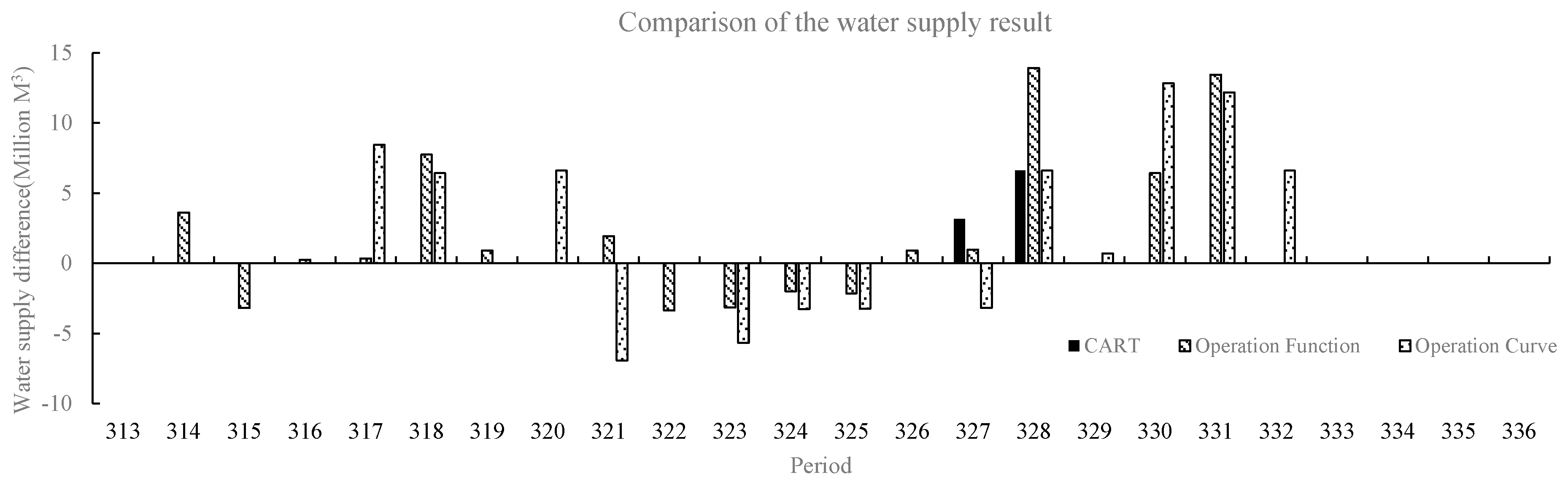
The operation decision of the operation chart is made based on the reservoir storage in the facing period and the operation period number, while the runoff is added as the decision-making basis in the operation function. The two operation rules cannot contain all of the factors that can affect the decision-making of the reservoir water supply, and more influencing factors need to be considered. Therefore, this study proposes a decision-making method for the multi-objective water supply reservoir operation by using data mining technology. Firstly, the optimal operation mode combination is determined by a dynamic programming (DP) model; then, the operation rules are extracted from the mapping relationship between the characteristic attributes and the combination of the optimal scheduling model, calculated by the Levenberg-Marquardt (LM) neural network and the classification and regression tree (CART); finally, the long-term continuous water supply is carried out with the operation rules, and the results are compared with those of the operation chart scheme and operation function scheme.

2. Methodology

The main process of knowledge discovery in databases (KDD) includes the data choice, establishment of the mapping relations, the data mining algorithm choice and the data mining of the extraction mode.

2.1. Data Choice of Operation Mode Mining

Data choice usually influences the operation mode mining effects. The influence factors of the operation mode decision contain three aspects: the condition of the reservoir, the task of the reservoir and the elements of the inflow. These three aspects reflect the relationship between supply and demand in the reservoir operation [23]. The characteristic attributes are chosen from these aspects, as shown below in Table 1.
(1) The condition of the reservoir
Reservoir storage (RS) is the most direct reaction of the conditions of the reservoir; it is the most important factor that impacts operation decisions. The bigger the storage, the greater the probability of normal water supply is; otherwise, the smaller the storage, the greater the probability of limiting water supply is.
(2) The task of the reservoir
The distribution of Water demand (WD) is uneven over a year, especially regarding the agricultural irrigation water. Limiting the water supply mostly occurred during periods in which the WD was high, while the potential of limiting the water supply is limited when the WD is low.
Operation period number (OPN) contains information about the degree of conflict between the runoff and water demand conditions. The operation horizon is one year of 12 periods, and each operation period is a calendar month in this study (N = 1, 2, …, 12). According to historical statistical data, runoff shows evident high- and low-flow changes during different periods within the year. Additionally, the water demand is obviously related to the period number; for example, irrigation water has strong seasonal characteristics.
(3) The elements of the inflow
Runoff (RO) is the key factor in the decision-making of the operation mode. The reservoir-available water includes two parts, one is the RS, the other is the period RO, and RO is the main source from which the reservoir supplies water.
Hydrological year type (HYT) can provide the information about the impact of the operation in the current period on the operation in the future period. Runoff has large differences in different hydrological years. Even if the other attributes are similar, operations in different hydrological years are obviously different from each other. For example, in low-flow years, even the reservoir storage water is high, so limiting the water supply ought to be established in advance. Conversely, it is not necessary to limit the water supply in high-flow years.

2.2. Establishment of the Mapping Relations

The establishment of the mapping relations between the characteristic attributes and the optimal operation modes is the core of data mining techniques. Reservoir operation is a multi-stage decision optimization problem, so the optimal operation modes can be solved by the dynamic programming (DP) model [23].

2.2.1. The Solution of the Optimal Operation Modes

The DP model mainly includes the following parts:
(1) Calculation variable
Stage variable: the calculation periods are used as the stages of the DP mode, so the time variable t is chosen as the stage variable.
State variable: the water storage capacity St at the beginning of the period t is chosen as the state variable, which can reflect the evolution of the operation process.
Decision variable: the decision variable of the DP model is Rt, namely the reservoir water supply during different periods. The pattern classification and rules of the water supply are shown in Table 2.
a 1 , a 2 , …, a N are hedging factors for different water demands, which are decided by respective demand elasticity ranges. N is the number of water supply targets. Currently, most reservoirs have multiple water supply targets, including water supplies for irrigation, industry, domestic usage, and the ecological environment. The priority and assurance rate of water supply targets are different. For example, industrial water has a high utilization rate, and it is sensitive to water deficit, so the demand elasticity range of the industrial water supply is small; however, irrigation water has low efficiency and a large elastic range.
(2) State transition equation:
R S t + 1 = R S t + R O t R t L t
where RSt, RSt+1 are the reservoir storage at the beginning and end of period t, respectively; ROt is the runoff flow; Lt is the reservoir leakage loss of evaporation.
(3) Main constraint
R S min R S t R S max
where RSmin, RSmax are the reservoir dead storage and upper limit storage, respectively.
(4) Operation objective
The operation objective is used to minimize the water deficit loss during the reservoir operation period. Actually, the convex function relation is found between the water deficit loss and the water shortage amount, except in the elasticity range of demand. Thus, the objective is to minimize the total water shortage during the operation period. The objective function is expressed as [24]:
min D I = t = 1 T ( R t i = 1 N W D i , t ) 2
(5) Recursion equation: the DP mode is calculated by the inverse time sequence recursive method, and the recursion equation is as follows:
{ D I t = 0 t = 1 D I t = min { F t ( R S t , R t ) + D I t 1 } t > 1
where F t ( R S t , R t ) is the calculated deficit index of the decision variable Rt under the reservoir storage condition RSt in the period t. DIt+1 is the cumulative value of the deficit index in period 1 to t + 1.

2.2.2. Mapping Relations

Through the combination of the characteristic attributes and the optimal operation model which is calculated by the deterministic optimal model (DP), the dataset for mining the operation pattern of the water supply is presented. Table 3 shows parts of the dataset.

2.3. Data Mining

2.3.1. Principle of the LM Network

A neural network has the abilities of self-learning, self-organization, and self-adaptation, and can obtain a network weight and structure through learning and training [
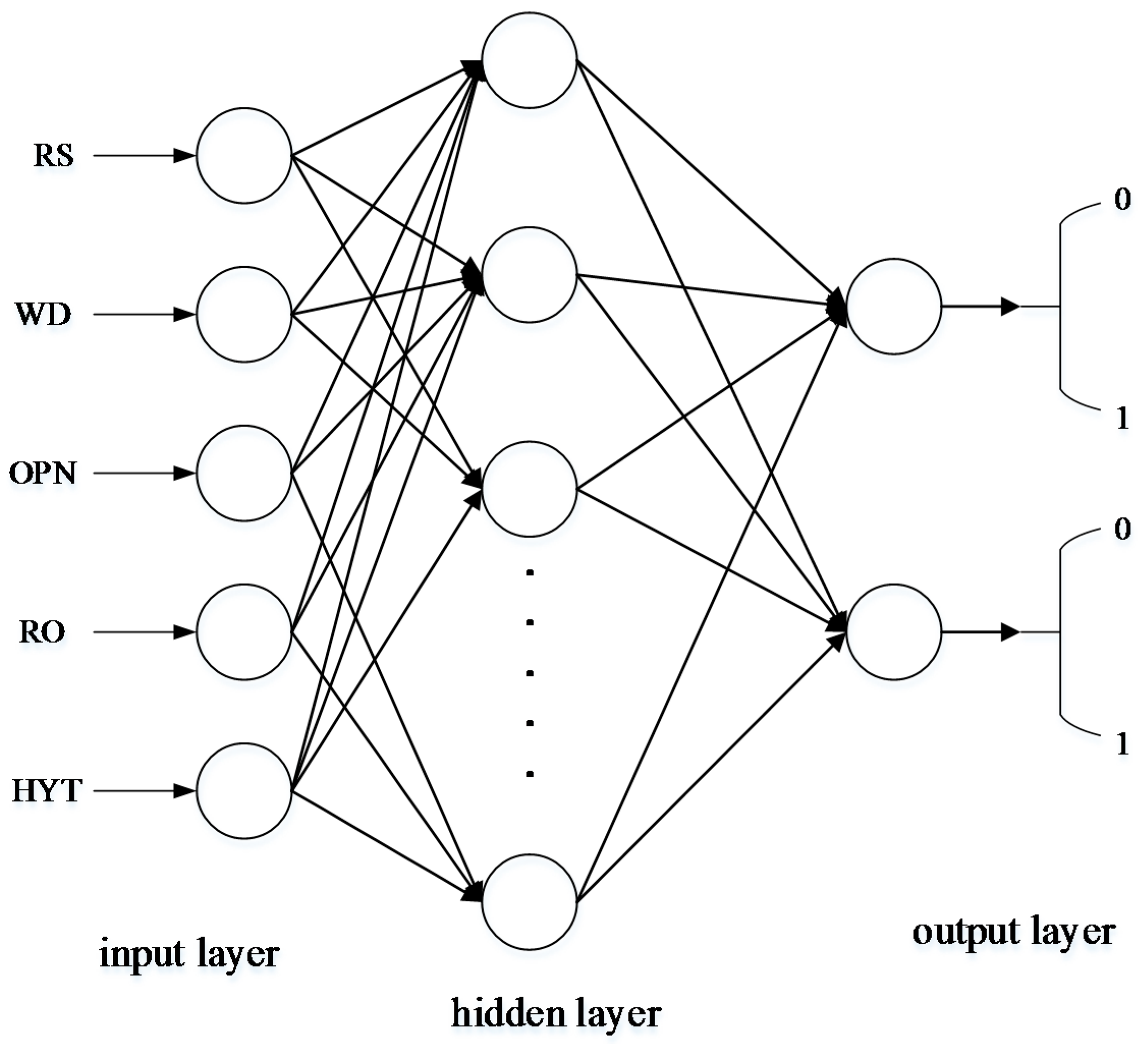
25]. A multi-level feed-forward neural network has the ability to approach any nonlinear continuous mapping in theory, which is very appropriate for model building and the controlling of nonlinear systems, and is the kind of neural network model that is usually applied. The common standard back propagation (BP) learning algorithm is a gradient descent method, whose parameter moves in the opposite direction of the error gradient, decreasing the error function until reaching the minimum value. The complexity of the calculation is mainly caused by the partial derivative. However, the linear convergence speed of this method, which is based on gradient descent, is very slow. The LM algorithm is the improved form of the Gaussian-Newton method, which has both the characteristics of the Gaussian-Newton method and the global characteristics of the gradient method. Due to using approximate second derivative information, the LM algorithm is faster than the gradient method. The structure of the LM network, which is shown in Figure 1, is designed as follows [26,27]:
(a)
The number of input layer nodes is five based on the number of characteristic attributes.
(b)
The number of output layer nodes is two, and the correspondence between the output and the operation model is shown in Table 4.
(c)
The number of hidden layer nodes is chosen based on the empirical formulas, which is shown as follows:
n = n i + n 0 + a
where n1 is the number of input layer nodes, n0 is the number of output layer nodes, a is a constant between 1 and 10, and the number of hidden layer nodes is six after the trial calculation.
(d)
The LM algorithm is chosen as the training algorithm.
(e)
Transfer function: S-type functions are chosen as the transfer functions.

2.3.2. Principle of CART Classification

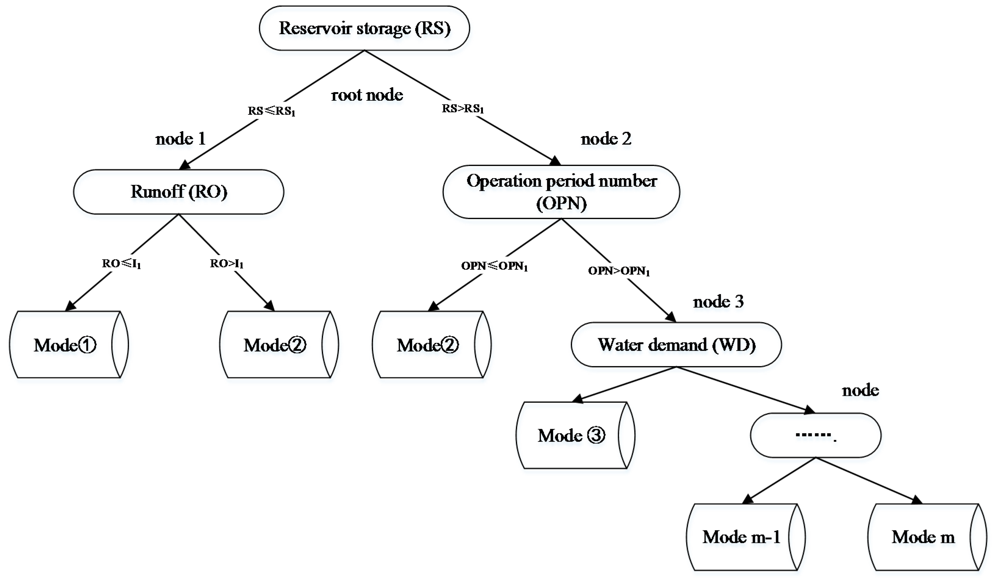
The recursive procedure is used to classify the observation set in the CART. The samples are segmented to minimize the impurity of the subset (the new sample), eventually creating a two-fork tree with a simple structure (Figure 2). The Gini coefficient is used as the index of the impurity measurement in this study.
(a) Definition of the index of impurity
The critical value is determined in the segmentation of the decision tree node, which is a basis for generating the sub-nodes. The determination of the critical value takes the Gini coefficient as the dividing index, which is defined as follows [28]:
Gini ( t ) = 1 i = 1 c p 2 ( j | t )
where Gini ( t ) is the Gini coefficient of node t, c is the number of the classification, and p ( j | t ) is the proportion of the j class in node t. When i ( t ) = 0, then all the samples belong to one class.
(b) The establishment of the CART
The establishment of the CART is a recursive procedure of creating a two-fork tree. At first, all of the observed values are located in the root node. Then a node is divided into the left and right two nodes by using the segmentation point. The result of the segmentation point is measured by the gain Δ i ( s , t ) , which is defined as the difference of impurity between the parent node and the sub-node [29]. It is calculated by the formula of goodness-of-split criteria as follows:
Δ i ( s , t ) = Gini ( t ) p L [ i ( t L ) ] p R [ i ( t R ) ]
where s represents a particular segmentation, p L , p R represent the proportion of the sample in the left and right child nodes, and i ( t L ) , i ( t R ) represent the impurity of the left and right child nodes.
The segmentation point with a maximum value of Δ i ( s , t ) is selected. The CART is built by repeating the above process.
(c) CART pruning
In the segmentation training, the number of samples available for selection will be fewer and fewer with the increase in the number of nodes. When the sample number is less than that of statistical significance, the estimated results will become unreliable, and will result in the phenomenon of over-fitting, reducing the generalizability of the CART. Thus, the CART needs to be pruned. In the study of decision-tree pruning, there are four kinds of pruning methods commonly used: PEP (pessimistic error pruning), MEP (minimum error pruning), CCP (cost-complexity pruning) and EBP (error-based pruning). CCP is used in this study.

3. Case Study

The 35-year long-series data from 1956 to 1990 of the Heiquan reservoir is chosen as the training dataset, and the 10-year long-series data from 1991 to 2000 is chosen as the test dataset. The mapping relations between the characteristic attributes and the optimal operation modes is built. The characteristic attributes include the reservoir storage, the operation period, the runoff, the storage water, and the hydrological years with the long-series data. The structure and parameters of the CART classifier and LM classifier are identified by learning the training dataset with class labels, namely the operation mode. The definition of the operation mode is shown in Table 5.

3.1. Training Results Analysis

There are 420 operation periods in the training sample, so each operation scheme is composed of 420 operation modes. The operation modes of the DP scheme are calculated by the inverse time sequence recursive method; the operation modes of the LM scheme and the CART scheme are obtained by the LM classifier and the CART classifier based on the characteristic attributes. In order to verify the accuracy of the LM classifier and the CART classifier, the optimal operation modes of the DP scheme need to be counted, and the statistical results are as follows: there are 168 operation mode ①, 96 operation mode ②, and 181 operation mode ③ instances during the 420 operation periods of the training samples. The LM classifier and the CART classifier are applied to the operation model classification of the training dataset. Statistical analysis is performed by the confusion matrix, as shown in Figure 3. Figure 3 shows the confusion matrix of the LM neural network. The classification correction rate of mode ① is 82.6% that of mode ② is 33.3%, and that of mode ③ is 85.5%, and the total correction rate is only 73.6% by using the LM classifier. This indicates that the classification result of the LM classifier is not reasonable, especially for the classification result of mode ②. The confusion matrix of the CART classifier shows that the classification correction rate of mode ① is 87.4%, that of mode ② is 77.0%, and that of mode ③ is 91.6%, and the total correction rate is 86.9%. This shows that the CART classifier has higher accuracy. The correction rate distribution of different operation modes in the training dataset is mode ③ > mode ② > mode ①, which has a positive relation with the sample number of the operation modes in the training samples.

3.2. Test Sample Analysis

Comparison and Analysis of Classifier Results of the Test Dataset

The LM classifier and the CART classifier are used for the classification of the test dataset. The confusion matrix of the CART classifier shows that the classification correction rate of mode ① is 90.9%, that of mode ② is 68.8%, and that of mode ③ is 93.4%, and the total correction rate is 83.3%, as shown in Figure 4. Compared with the correction rate of the training dataset, the correction rates of the two classifiers for the test dataset both decrease. This is because although the statistic characteristics of the characteristic attributes of the training sample correspond with that of the test sample, there are some differences between the two samples. The classification correction rate is limited by the number of training samples, and the mutagenesis data of the test sample have an effect on the classification correction rate. Therefore, the correction rate of the training sample is higher than that of the test sample, and increasing the number of the test samples can improve the correction rate of the classifiers effectively.
The receiver operating characteristic (ROC) curve takes each value of the prediction results as the possible judging threshold, and the corresponding sensitivity and specificity are obtained. The fake positive rate (specificity) is taken as the X-axis, and the true positive rate (sensitivity) is taken as the Y-axis. The area under the curve (AUC) is chosen as the measure index for model prediction accuracy, whose range is [0, 1]. The higher the value of the AUC is, the stronger the judgment of the classifier will be. As can be seen from Figure 5, the corresponding ROC curve of the CART classifier is near the left corner, and the calculated AUC values of the three types of operation model of the CART classifier are 0.901, 0.813, and 0.925, respectively. The classification AUC values of the CART classifier for mode ① and mode ③ both reach high levels (AUC > 0.9), and the classification AUC value for mode ② also reaches a middle level. Consequently, the CART classifier has greater accuracy for the classification of the operation modes.

3.3. Long-Series Result Analysis

Through the analysis of training results and test samples, the classification results of the CART classifier are better than those of the LM classifier. Thus, the CART classifier is chosen to guide the reservoir long-series operation, and the operation result is used for comparison with the results of other operation methods, including the DP, operation chart (OC), and operation function (OF) [23]. The operation area is separated into three areas by the line of the operation chart, and each area corresponds with one kind of operation mode. The operation function is obtained from the multi-element linear regression method.
The long-series regulation calculation for the Heiquan reservoir is carried out based on the monthly inflow data from 1956 to 2000 by using the CART classifier, operation chart, operation function, and DP model. During the calculation adjustment process of the long-series, the earlier decisions will influence the later initial conditions, and it is difficult to judge the advantages and disadvantages of the operation schemes through the classification correction rate. Thus, the water deficit index, which is used as the objective function of the deterministic optimal model, is chosen as the evaluation index, and the water deficit index results are shown in Table 6.
The DP model is one optimum model; it divides the reservoir storage process into several parts, utilizes a step-by-step inducing principle to make decisions on every part, and then gets the optimal operation performance of the total problem. So the water deficit index obtained from the DP model is the smallest. The water deficit indexes of the operation chart scheme, the operation function scheme, and the CART scheme are 6.33, 5.92, and 4.38, respectively. The index of the CART scheme is the closest to the optimum scheme (DP scheme).
According to the analysis of the long-series operation results, at the beginning of the 313rd period (January 1982), the initial reservoir storage obtained from different schemes was similar. The water supply results of the dry year can be used to analyze the advantages and disadvantages of different operation schemes better, so the 24 operation periods between 1982 and 1983 are chosen as the study objectives. Since the water supply process of the DP scheme is optimal, the smaller the difference of the water supply process between the DP scheme and the operation scheme, the better the operation scheme is. The comparison analysis of the water supply results shows that the water supply of the CART scheme is almost the same as that of the DP scheme. The difference of the water supply between the DP scheme and the other operation schemes is shown in Figure 6, which shows that the water supply process with the greatest difference is the OC scheme, and then the OF scheme. This is in agreement with the results shown in Table 6.
The operation modes of different operation schemes during periods 321–332 are shown in Table 7. There are three misclassifications in the CART scheme, which happened, respectively, in period 325, period 327, and period 328; the difference value of the misclassification is only 1. Deep damages occurred in the OF scheme and OC scheme. Especially in the OC scheme, deep damage happened in May and June, which were both water usage high points. The year 1982 was a dry year, and the inflow of the Heiquan reservoir was less than that of normal years after the flood season. However, the reservoir storage at the beginning of the decision period is the only decision-making factor, there are no water supply restricting measures after the flood season in the OF scheme and OC scheme. Instead, the influence of the later inflow is taken into account in the CART scheme, so the water is supplied in mode ② after the flood season from October to December. Impounding in advance avoids the later deep damage. There is no deep damage in the CART scheme, which indicates that the CART scheme can guide the reservoir water supply operation effectively.

4. Conclusions

This paper chose two data mining technologies—the CART decision tree and the LM artificial neural network—to apply to water supply operation. The traditional extraction problem of the reservoir operation rules is translated into a data mining problem. Firstly, the optimal model of reservoir water supply operation is established by the DP model, so the optimal operation model of long-series scheduling is obtained. Then, the reservoir storage, runoff, water demand, operation period number, and hydrological year are chosen as the reservoir status dataset, and the mapping relation between the status dataset and optimal operation mode is established. Finally, the CART classifier and LM classifier are built based on the mapping relation. The results are summarized below:
(1)
The classification results of the training dataset are better than those of the test dataset, and the classification effect of the CART is better than that of the LM. The correction rate of the CART test sample is 83.3%. The classification values of the CART classifier for mode ① and mode ③ both reach a high value (ACU > 0.9), and the classification result for mode ②reaches the middle level.
(2)
Through a comparison of the results of the long series of reservoir water supply operation, which is guided by the DP, CART, OC, and OF, we see that the deficit index of the CART scheme is closest to the optimal operation mode and the deep damage is efficiently avoided. This indicates that the modes which are distinguished by the CART can guide the reservoir water supply operation effectively.

Author Contributions

Yi Ji designed the experiments and wrote the manuscript; Xiaohui Lei provided suggestions on the data analysis and manuscript preparation, Siyu Cai and Xu Wang revised the manuscript.

Conflicts of Interest

The authors declare no conflict of interest.

References

  1. Zeng, X.; Hu, T.; Guo, X.; Li, X. Water transfer triggering mechanism for multi-reservoir operation in inter-basin water transfer-supply project. Water Resour. Manag. 2014, 28, 1293–1308. [Google Scholar] [CrossRef]
  2. Peng, Y.; Chu, J.; Peng, A.; Zhou, H. Optimization operation model coupled with improving water-transfer rules and hedging rules for inter-basin water transfer-supply systems. Water Resour. Manag. 2015, 29, 3787–3806. [Google Scholar] [CrossRef]
  3. Birhanu, K.; Alamirew, T.; Olumana Dinka, M.; Ayalew, S.; Aklog, D. Optimizing reservoir operation policy using chance constraint nonlinear programming for koga irrigation dam, ethiopia. Water Resour. Manag. 2014, 28, 4957–4970. [Google Scholar] [CrossRef]
  4. Jothiprakash, V.; Shanthi, G. Single reservoir operating policies using genetic algorithm. Water Resour. Manag. 2006, 20, 917–929. [Google Scholar] [CrossRef]
  5. Zhao, T.; Zhao, J. Improved multiple-objective dynamic programming model for reservoir operation optimization. J. Hydroinform. 2014, 16, 1142–1157. [Google Scholar] [CrossRef]
  6. Bower, B.T.; Hufschmidt, M.M.; Reedy, W.W. Operating procedures: Their role in the design of water-resource systems by simulation analyses. In Design of Water Resource Systems; Harvard University Press: Cambridge, MA, USA, 1962; pp. 443–458. [Google Scholar]
  7. Clark, E.J. Impounding reservoirs. J. Am. Water Works Assoc. 1956, 48, 349–354. [Google Scholar]
  8. Maass, A.; Hufschmidt, M.M.; Dorfman, R.; Thomas, H.A.; Marglin, S.A.; Fair, G.M.; Bower, B.T.; Reedy, W.W.; Manzer, D.F.; Barnett, M.P.; et al. Design of water resource system. Water Resour. Res. 1962, 94, 329–336. [Google Scholar]
  9. Tu, M.-Y.; Hsu, N.-S.; Tsai, F.T.-C.; Yeh, W.W.-G. Optimization of hedging rules for reservoir operations. J. Water Resour. Plan. Manag. 2008, 134, 3–13. [Google Scholar] [CrossRef]
  10. Chen, L. A Study of Optimizing the Rule Curve of Reservoir Using Object Oriented Genetic Algorithms. Ph.D. Thesis, Department of Agricultural Engineering, National Taiwan University, Taipei, Taiwan, 1995. [Google Scholar]
  11. Oliveira, R.; Loucks, D.P. Operating rules for multireservoir systems. Water Resour. Res. 1997, 33, 839–852. [Google Scholar] [CrossRef]
  12. Chang, F.J.; Chen, L.; Chang, L.C. Optimizing the reservoir operating rule curves by genetic algorithms. Hydrol. Process. 2005, 19, 2277–2289. [Google Scholar] [CrossRef]
  13. Chen, L.; McPhee, J.; Yeh, W.W.-G. A diversified multiobjective ga for optimizing reservoir rule curves. Adv. Water Resour. 2007, 30, 1082–1093. [Google Scholar] [CrossRef]
  14. Tu, M.-Y.; Hsu, N.-S.; Yeh, W.W.-G. Optimization of reservoir management and operation with hedging rules. J. Water Resour. Plan. Manag. 2003, 129, 86–97. [Google Scholar] [CrossRef]
  15. Ai, X.; Gao, Z. Combined optimal method of drawing reservoir optimal operation figure. In Advances in Computer Science, Intelligent System and Environment; Springer: Berlin/Heidelberg, Germany, 2011; pp. 103–107. [Google Scholar]
  16. Guo, X.; Hu, T.; Zeng, X.; Li, X. Extension of parametric rule with the hedging rule for managing multireservoir system during droughts. J. Water Resour. Plan. Manag. 2012, 139, 139–148. [Google Scholar] [CrossRef]
  17. Bhaskar, N.R.; Whitlatch, E.E. Derivation of monthly reservoir release policies. Water Resour. Res. 1980, 16, 987–993. [Google Scholar] [CrossRef]
  18. Karamouz, M.; Houck, M.H. Annual and monthly reservoir operating rules generated by deterministic optimization. Water Resour. Res. 1982, 18, 1337–1344. [Google Scholar] [CrossRef]
  19. Karamouz, M.; Houck, M.H.; Delleur, J.W. Optimization and simulation of multiple reservoir systems. J. Water Resour. Plan. Manag. 1992, 118, 71–81. [Google Scholar] [CrossRef]
  20. Wang, Y.-M.; Chang, J.-X.; Huang, Q. Simulation with RBF neural network model for reservoir operation rules. Water Resour. Res. 2010, 24, 2597–2610. [Google Scholar] [CrossRef]
  21. Karamouz, M.; Ahmadi, A.; Moridi, A. Probabilistic reservoir operation using bayesian stochastic model and support vector machine. Adv. Water Resour. 2009, 32, 1588–1600. [Google Scholar] [CrossRef]
  22. Mehta, R.; Jain, S.K. Optimal operation of a multi-purpose reservoir using neuro-fuzzy technique. Water Resour. Res. 2009, 23, 509–529. [Google Scholar] [CrossRef]
  23. Yin, Z.J.; Wang, X.L.; Hu, T.S.; Wu, Y.Q. Water supply reservoir operating rules extraction based on data mining. Syst. Eng. Theory Pract. 2006, 26, 129–135. [Google Scholar]
  24. Xu, T.Y.; Qin, X.S. A sequential fuzzy model with general-shaped parameters for water supply–demand analysis. Water Resour. Manag. 2015, 29, 1431–1446. [Google Scholar] [CrossRef]
  25. Piotrowski, A.P.; Napiorkowski, J.J. Optimizing neural networks for river flow forecasting—Evolutionary computation methods versus the levenberg–marquardt approach. J. Hydrol. 2011, 407, 12–27. [Google Scholar] [CrossRef]
  26. Adeloye, A.J.; Munari, A.D. Artificial neural network based generalized storage–yield–reliability models using the levenberg–marquardt algorithm. J. Hydrol. 2006, 326, 215–230. [Google Scholar] [CrossRef]
  27. Nowak, W.; Cirpka, O.A. A modified levenberg–marquardt algorithm for quasi-linear geostatistical inversing. Adv. Water Resour. 2004, 27, 737–750. [Google Scholar] [CrossRef]
  28. Speybroeck, N. Classification and Regression Trees; Chapman & Hall/CRC: Boca Raton, FL, USA, 1998; pp. 1174–1176. [Google Scholar]
  29. Bessler, F.T.; Savic, D.A.; Walters, G.A. Water reservoir control with data mining. J. Water Resour. Plan. Manag. 2003, 129, 26–34. [Google Scholar] [CrossRef]
Figure 1. The structure of the LM network.
Water 08 00599 g001
Figure 2. The diagram of the CART.
Water 08 00599 g002
Figure 3. The confusion matrix of the LM classifier and the CART classifier for the training dataset. (a) The confusion matrix of the LM classifier; (b) The confusion matrix of the CART classifier.
Water 08 00599 g003
Figure 4. The confusion matrix of the LM classifier and the CART classifier for the test dataset.
Water 08 00599 g004
Figure 5. The ROC and AUC results of the test dataset.
Water 08 00599 g005
Figure 6. Comparison of water supply results.
Water 08 00599 g006
Table 1. The classification of characteristic attributes.
Condition of the ReservoirTask of the ReservoirElements of Inflow
Reservoir storage (RS)Water demand (WD)Runoff (RO)
Operation period number (OPN)Hydrological year type (HYT)
Table 2. The pattern classification and rules of the water supply.
Operation ModeLimit TargetWater Supply
1None R t = W D 1 , t + W D 2 , t + + W D N , t
2 D 1 , t R t = ( 1 a 1 ) W D 1 , t + W D 2 , t + + W D N , t
3 D 1 , t , D 2 , t R t = ( 1 a 1 ) W D 1 , t + ( 1 a 2 ) W D 2 , t + + W D N , t
N + 1 D 1 , t , D 2 , t , …, D N , t R t = ( 1 a 1 ) W D 1 , t + ( 1 a 2 ) W D 2 , t + + ( 1 a N ) W D N , t
Table 3. The parts of the dataset for mining the operation pattern of the water supply.
No.Characteristic AttributesOptimal Operation Model
Condition of the ReservoirTask of the ReservoirElements of Inflow
RSWDOPNROHYT
1179263.749685.67345882
1188656.3110280.62167382
1197320.56811270.51283482
1206320.6712412.12163182
1213429.6011320.45261643
Table 4. The corresponding relationship between the network output and the operation model.
Output(0,0)(0,1)(1,0)
Operation Model
Table 5. The definition of the operation mode.
Operation ModeLimit TargetWater Supply
None R t = D 1 , t + D 2 , t
D 1 , t R t = ( 1 0.2 ) D 1 , t + D 2 , t
D 1 , t , D 2 , t R t = ( 1 0.2 ) D 1 , t + ( 1 0.1 ) D 2 , t
Notes: D 1 , t represents the water demand for agricultural irrigation in the period t; D 2 , t represents the water demand of the urban supply in period t.
Table 6. Water deficit index of different operation rules.
IndexOperation ChartOperation FunctionCARTDP
Water deficit index6.335.924.383.62
Table 7. Operation modes of different operation schemes.
Period321322323324325326327328329330331332
MonthSeptemberOctoberNovemberDecemberJanuaryFebruaryMarchAprilMayJuneJulyAugust
DP
CART
OF--
OC--
Notes: ①, ②, and ③ in the table represent three operation modes, respectively; - represents the deep damage.

