1. Introduction
In recent years, the increasing conflicts of water demand and supply have promoted a greater need for reasonable water resource development and management [
1,
2,
3,
4]. Currently, the operation target for a reservoir has shifted from single objective to multi-objective, including agricultural irrigation, industry, urban supply, and even river ecology. The assurance rate and priority are different between each water supply target [
5]. Under uncertain stream flow and multi-objective demands, water allocation processes have become more complex. Consequently, it is necessary to conduct the decision analysis of multi-objective water supply for reservoirs and build a convenient water supply decision-making model that is practical for administrative staff to use.
In order to reasonably distribute water resources, many water supply operation rules are put forward, including the space rule [
6], the New York rule [
7], the pack rule [
8], the hedging rule [
9], and so on. Water supply operation rules are generally expressed by different forms of water supply operation charts (OC) or operation functions (OF). A reservoir operation chart is a control graph to guide reservoir operations, which uses time (month, 10 days) as the
X-axis and the reservoir water level or storage water as the
Y-axis. The graph separates the reservoir storage capacity into different water supply areas according to the indicating lines that control the reservoir storage and supply, which is a main tool for guiding reservoir operations. Research about water supply operation charts mainly starts around determining the method of the operation chart, the efficiency of the algorithm, and the equilibrium relationship between the reservoir water supply and other beneficial objectives. Chen et al. [
10,
11] applied a genetic algorithm in the making of an optimal operation chart of a single-objective reservoir. Chang et al. [
12] compared and analyzed the influence of real number encoding and binary encoding on the optimal application of a multi-objective Genetic Algorithm (GA) in a reservoir operation chart. They proposed that real number encoding had higher computational efficiency and precision. Chen et al. [
13] built a macroevolution multi-objective, and studied the operation chart of a multipurpose reservoir in Taiwan. Application research of other optimization algorithms includes that of Tu et al. [
14], who studied the influence of the current storage water level on operation rules of multi-objective reservoirs. Ai et al. [
15] used a POA (progress optimality algorithm) to optimize the number and location of scheduling lines and water supply amounts in different partitions, and then determined reasonable and effective reservoir operation rules. Guo et al. [
16] combined parameter rules with operation rules, built simulation models by using particle swarm optimization, applied it in reservoir group optimal operations under dry conditions, and then obtained a group of scheduling lines.
The optimal operation function is usually determined by using an implicit stochastic method [
17]. According to historical long-series data, the optimum operation process sample can be obtained by using a deterministic optimization method, and then the optimum decision rules can be obtained based on the statistical analysis for this sample, namely the operation function. This operation function, obtained by fitting optimal samples, needs to be verified and adjusted through the simulation operation, namely the “optimization-simulation-re-optimization” framework [
18]. The simulation is not only based on the measured hydrological series, but also based on runoff series produced by hydrological stochastic simulation technology, in order to further test and evaluate the operation function efficiency [
19]. The operation function can guide reservoir operation by building the function relationship between the reservoir water supply during the facing period (decision variable) and the current storage water and reservoir inflow in the facing period (state variable). The operation function research is mainly based on regression analysis, artificial intelligence algorithms, and a combination of other operation rules. Wang et al. [
20] used an artificial neural network to solve the reservoir water supply operation function and found that its nonlinear mapping ability could better reflect the complex relationship between independent variables and dependent variables in reservoir operation. Karamouz et al. [
21], aimed at the complexity and nonlinearity of the operation function, adopted support vector machine technology to build the reservoir optimal operation function, and proved the effectiveness of this method. The fuzzy system stored knowledge in the way of rules, adopted a group of fuzzy rules to describe the object’s characteristics, and solved uncertain problems through fuzzy logical deductions. Mehta and Jain [
22] used fuzzy technology to derive abstract reservoir operation rules and compared the effectiveness of three different kinds of fuzzy rules.
The operation decision of the operation chart is made based on the reservoir storage in the facing period and the operation period number, while the runoff is added as the decision-making basis in the operation function. The two operation rules cannot contain all of the factors that can affect the decision-making of the reservoir water supply, and more influencing factors need to be considered. Therefore, this study proposes a decision-making method for the multi-objective water supply reservoir operation by using data mining technology. Firstly, the optimal operation mode combination is determined by a dynamic programming (DP) model; then, the operation rules are extracted from the mapping relationship between the characteristic attributes and the combination of the optimal scheduling model, calculated by the Levenberg-Marquardt (LM) neural network and the classification and regression tree (CART); finally, the long-term continuous water supply is carried out with the operation rules, and the results are compared with those of the operation chart scheme and operation function scheme.
2. Methodology
The main process of knowledge discovery in databases (KDD) includes the data choice, establishment of the mapping relations, the data mining algorithm choice and the data mining of the extraction mode.
2.1. Data Choice of Operation Mode Mining
Data choice usually influences the operation mode mining effects. The influence factors of the operation mode decision contain three aspects: the condition of the reservoir, the task of the reservoir and the elements of the inflow. These three aspects reflect the relationship between supply and demand in the reservoir operation [
23]. The characteristic attributes are chosen from these aspects, as shown below in
Table 1.
(1) The condition of the reservoir
Reservoir storage (RS) is the most direct reaction of the conditions of the reservoir; it is the most important factor that impacts operation decisions. The bigger the storage, the greater the probability of normal water supply is; otherwise, the smaller the storage, the greater the probability of limiting water supply is.
(2) The task of the reservoir
The distribution of Water demand (WD) is uneven over a year, especially regarding the agricultural irrigation water. Limiting the water supply mostly occurred during periods in which the WD was high, while the potential of limiting the water supply is limited when the WD is low.
Operation period number (OPN) contains information about the degree of conflict between the runoff and water demand conditions. The operation horizon is one year of 12 periods, and each operation period is a calendar month in this study (N = 1, 2, …, 12). According to historical statistical data, runoff shows evident high- and low-flow changes during different periods within the year. Additionally, the water demand is obviously related to the period number; for example, irrigation water has strong seasonal characteristics.
(3) The elements of the inflow
Runoff (RO) is the key factor in the decision-making of the operation mode. The reservoir-available water includes two parts, one is the RS, the other is the period RO, and RO is the main source from which the reservoir supplies water.
Hydrological year type (HYT) can provide the information about the impact of the operation in the current period on the operation in the future period. Runoff has large differences in different hydrological years. Even if the other attributes are similar, operations in different hydrological years are obviously different from each other. For example, in low-flow years, even the reservoir storage water is high, so limiting the water supply ought to be established in advance. Conversely, it is not necessary to limit the water supply in high-flow years.
2.2. Establishment of the Mapping Relations
The establishment of the mapping relations between the characteristic attributes and the optimal operation modes is the core of data mining techniques. Reservoir operation is a multi-stage decision optimization problem, so the optimal operation modes can be solved by the dynamic programming (DP) model [
23].
2.2.1. The Solution of the Optimal Operation Modes
The DP model mainly includes the following parts:
(1) Calculation variable
Stage variable: the calculation periods are used as the stages of the DP mode, so the time variable t is chosen as the stage variable.
State variable: the water storage capacity St at the beginning of the period t is chosen as the state variable, which can reflect the evolution of the operation process.
Decision variable: the decision variable of the DP model is
Rt, namely the reservoir water supply during different periods. The pattern classification and rules of the water supply are shown in
Table 2.
, , …, are hedging factors for different water demands, which are decided by respective demand elasticity ranges. N is the number of water supply targets. Currently, most reservoirs have multiple water supply targets, including water supplies for irrigation, industry, domestic usage, and the ecological environment. The priority and assurance rate of water supply targets are different. For example, industrial water has a high utilization rate, and it is sensitive to water deficit, so the demand elasticity range of the industrial water supply is small; however, irrigation water has low efficiency and a large elastic range.
(2) State transition equation:
where
RSt,
RSt+1 are the reservoir storage at the beginning and end of period
t, respectively;
ROt is the runoff flow;
Lt is the reservoir leakage loss of evaporation.
(3) Main constraint
where
RSmin,
RSmax are the reservoir dead storage and upper limit storage, respectively.
(4) Operation objective
The operation objective is used to minimize the water deficit loss during the reservoir operation period. Actually, the convex function relation is found between the water deficit loss and the water shortage amount, except in the elasticity range of demand. Thus, the objective is to minimize the total water shortage during the operation period. The objective function is expressed as [
24]:
(5) Recursion equation: the DP mode is calculated by the inverse time sequence recursive method, and the recursion equation is as follows:
where
is the calculated deficit index of the decision variable
Rt under the reservoir storage condition
RSt in the period
t.
DIt+1 is the cumulative value of the deficit index in period 1 to
t + 1.
2.2.2. Mapping Relations
Through the combination of the characteristic attributes and the optimal operation model which is calculated by the deterministic optimal model (DP), the dataset for mining the operation pattern of the water supply is presented.
Table 3 shows parts of the dataset.
2.3. Data Mining
2.3.1. Principle of the LM Network
A neural network has the abilities of self-learning, self-organization, and self-adaptation, and can obtain a network weight and structure through learning and training [
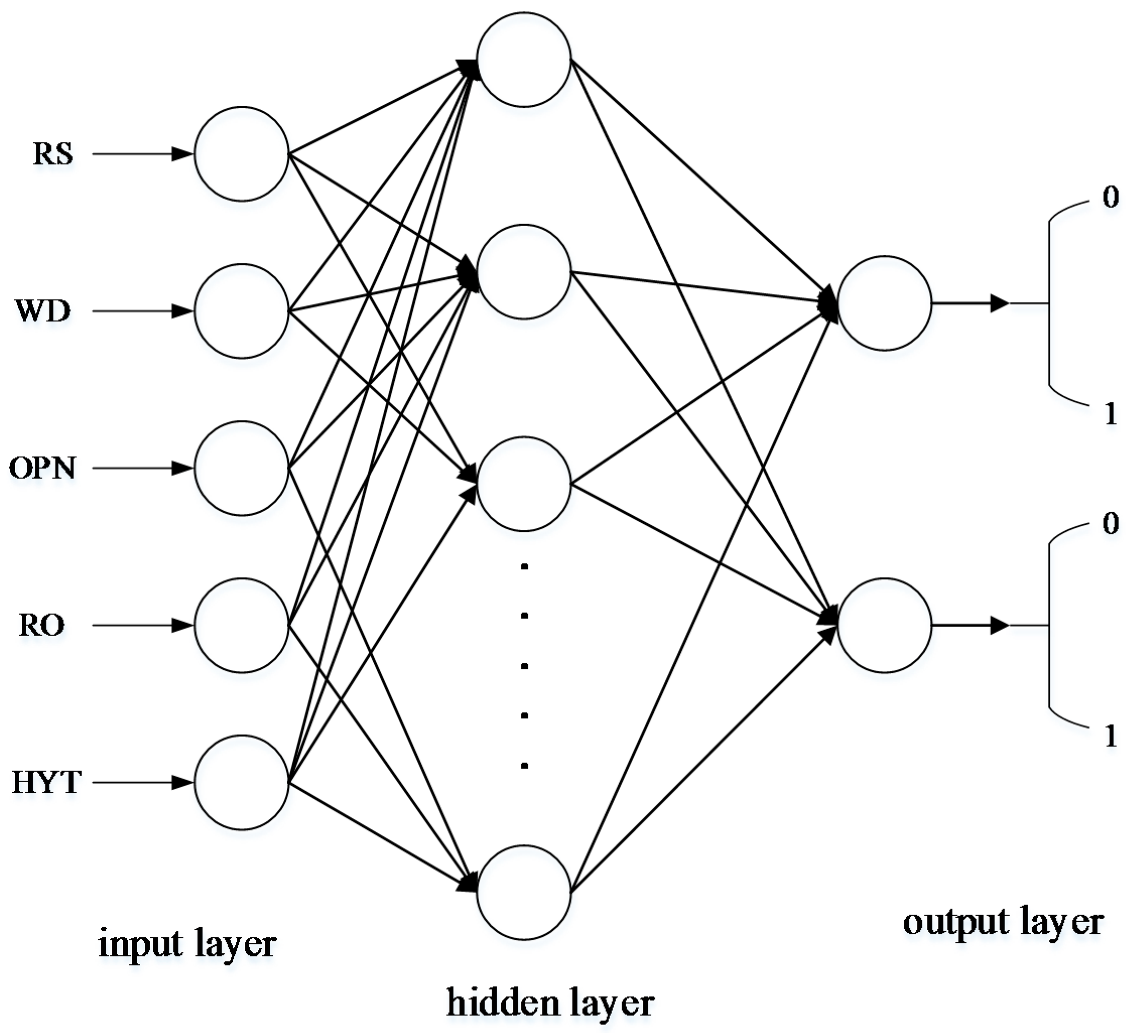
25]. A multi-level feed-forward neural network has the ability to approach any nonlinear continuous mapping in theory, which is very appropriate for model building and the controlling of nonlinear systems, and is the kind of neural network model that is usually applied. The common standard back propagation (BP) learning algorithm is a gradient descent method, whose parameter moves in the opposite direction of the error gradient, decreasing the error function until reaching the minimum value. The complexity of the calculation is mainly caused by the partial derivative. However, the linear convergence speed of this method, which is based on gradient descent, is very slow. The LM algorithm is the improved form of the Gaussian-Newton method, which has both the characteristics of the Gaussian-Newton method and the global characteristics of the gradient method. Due to using approximate second derivative information, the LM algorithm is faster than the gradient method. The structure of the LM network, which is shown in
Figure 1, is designed as follows [
26,
27]:
- (a)
The number of input layer nodes is five based on the number of characteristic attributes.
- (b)
The number of output layer nodes is two, and the correspondence between the output and the operation model is shown in
Table 4.
- (c)
The number of hidden layer nodes is chosen based on the empirical formulas, which is shown as follows:
where
n1 is the number of input layer nodes,
n0 is the number of output layer nodes,
a is a constant between 1 and 10, and the number of hidden layer nodes is six after the trial calculation.
- (d)
The LM algorithm is chosen as the training algorithm.
- (e)
Transfer function: S-type functions are chosen as the transfer functions.
2.3.2. Principle of CART Classification
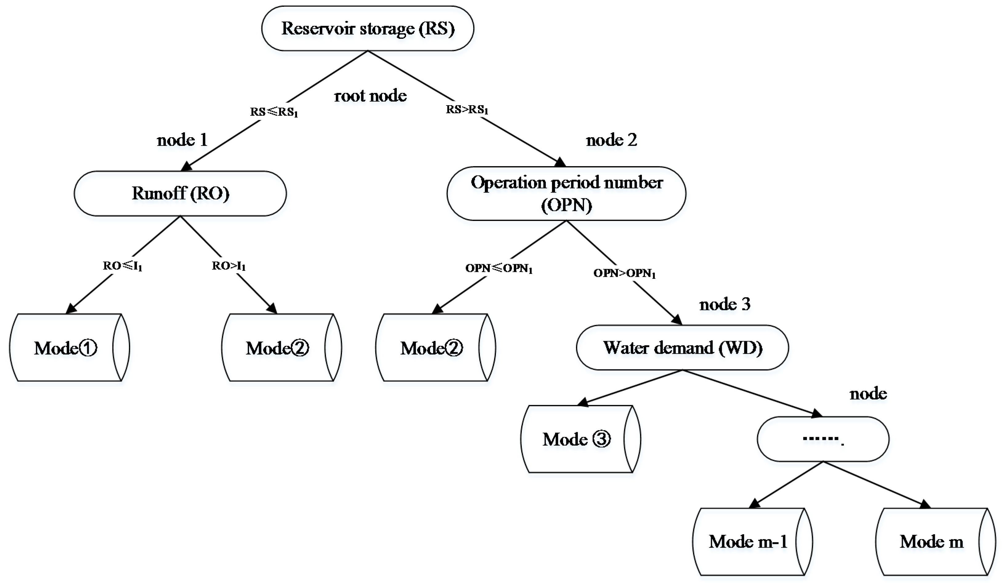
The recursive procedure is used to classify the observation set in the CART. The samples are segmented to minimize the impurity of the subset (the new sample), eventually creating a two-fork tree with a simple structure (
Figure 2). The Gini coefficient is used as the index of the impurity measurement in this study.
(a) Definition of the index of impurity
The critical value is determined in the segmentation of the decision tree node, which is a basis for generating the sub-nodes. The determination of the critical value takes the Gini coefficient as the dividing index, which is defined as follows [
28]:
where
is the Gini coefficient of node
t,
c is the number of the classification, and
is the proportion of the
j class in node t. When
= 0, then all the samples belong to one class.
(b) The establishment of the CART
The establishment of the CART is a recursive procedure of creating a two-fork tree. At first, all of the observed values are located in the root node. Then a node is divided into the left and right two nodes by using the segmentation point. The result of the segmentation point is measured by the gain
, which is defined as the difference of impurity between the parent node and the sub-node [
29]. It is calculated by the formula of goodness-of-split criteria as follows:
where
s represents a particular segmentation,
,
represent the proportion of the sample in the left and right child nodes, and
,
represent the impurity of the left and right child nodes.
The segmentation point with a maximum value of is selected. The CART is built by repeating the above process.
(c) CART pruning
In the segmentation training, the number of samples available for selection will be fewer and fewer with the increase in the number of nodes. When the sample number is less than that of statistical significance, the estimated results will become unreliable, and will result in the phenomenon of over-fitting, reducing the generalizability of the CART. Thus, the CART needs to be pruned. In the study of decision-tree pruning, there are four kinds of pruning methods commonly used: PEP (pessimistic error pruning), MEP (minimum error pruning), CCP (cost-complexity pruning) and EBP (error-based pruning). CCP is used in this study.
