
Water Balance and Level Change of Lake Babati, Tanzania: Sensitivity to Hydroclimatic Forcings

 , and
, and 
Abstract
:1. Introduction
2. Materials and Methods
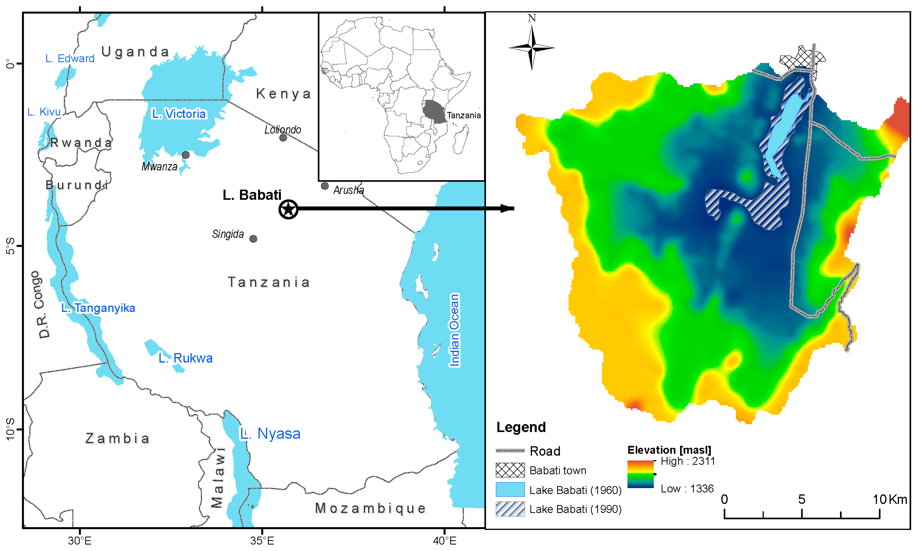
2.1. Description of the Study Site
2.1.1. General
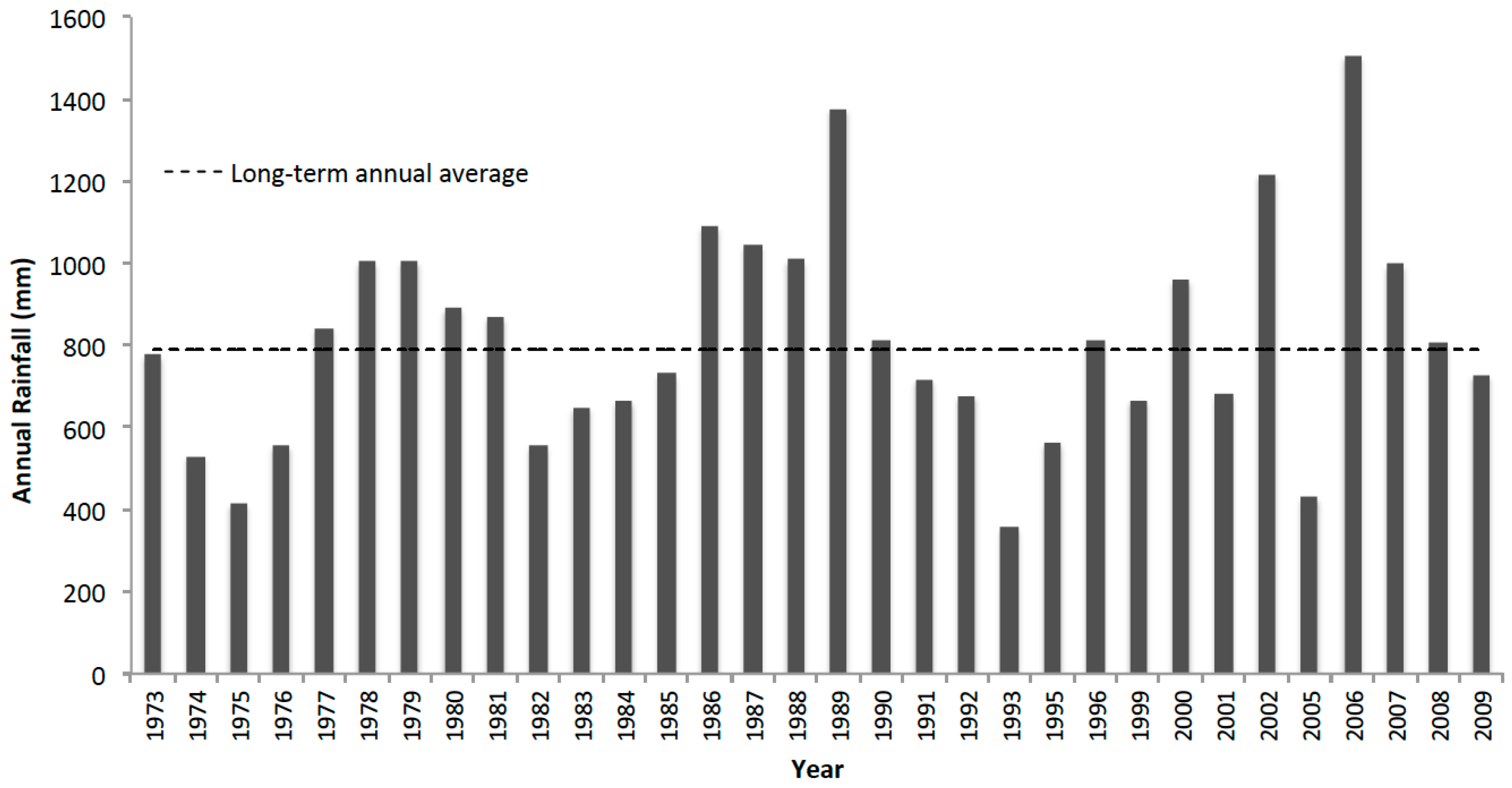
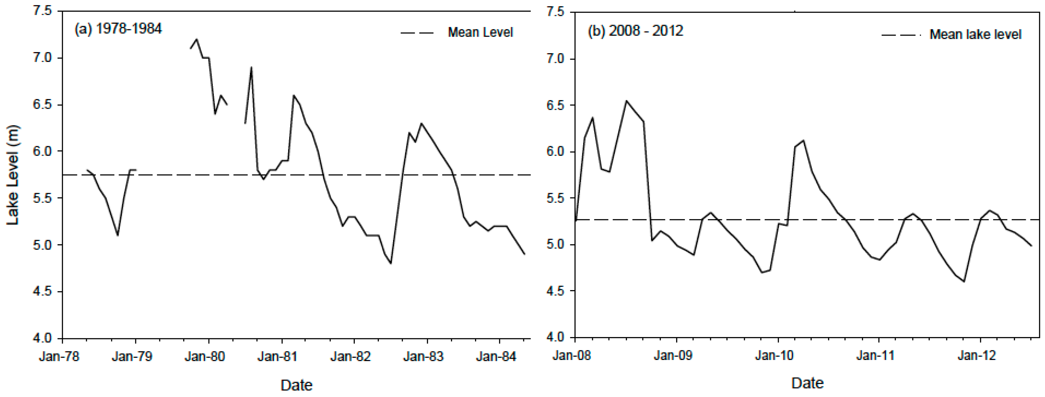
2.1.2. Hydroclimatic Conditions and Independent Observations of Water Balance Components
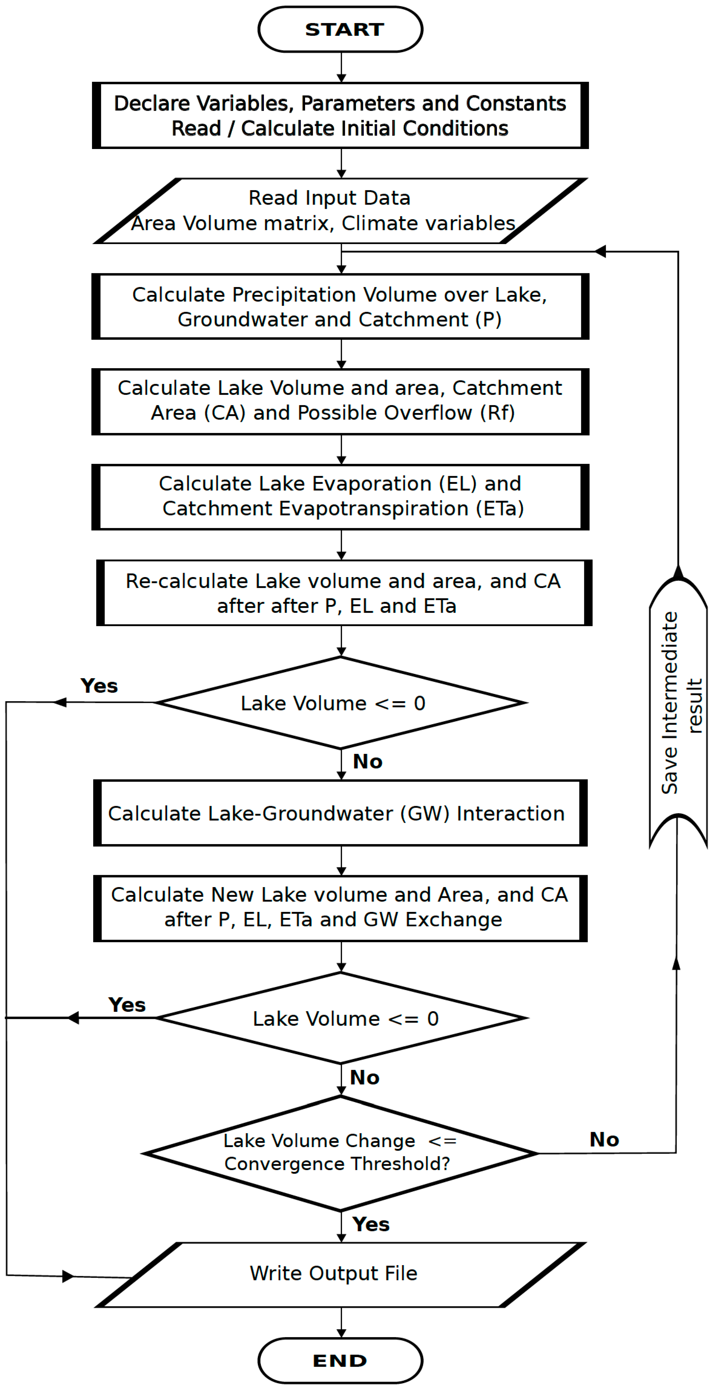
2.2. The Lake Water Balance Model
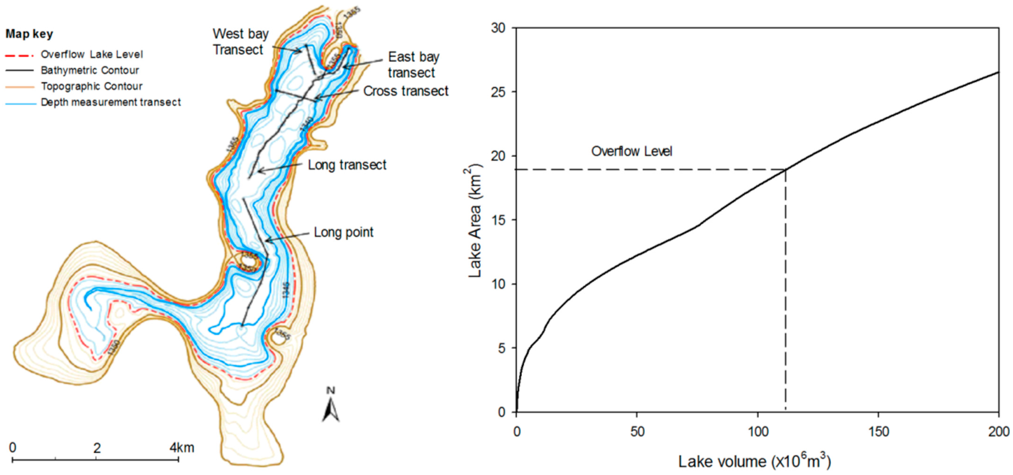
2.2.1. Catchment Topography and Lake Bathymetry
2.2.2. Evaporation over the Lake
2.2.3. Evapotranspiration over the Groundwater Reservoir and the Catchment
2.2.4. Groundwater-Lake Water Interaction
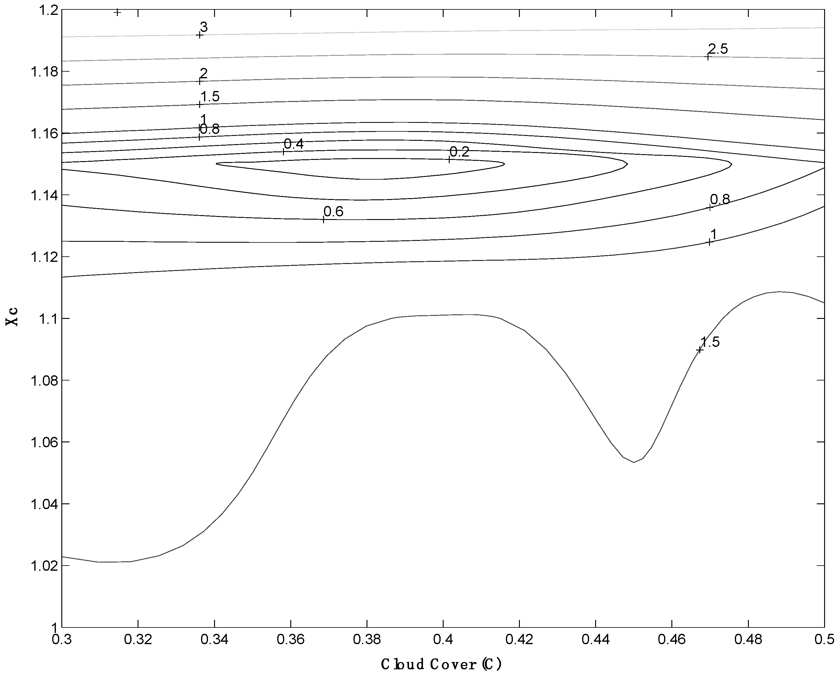
2.3. Model Structure, Input Parameters, Calibration, and Sensitivity
2.4. Assessment of Future Climatic Conditions
3. Results and Discussion
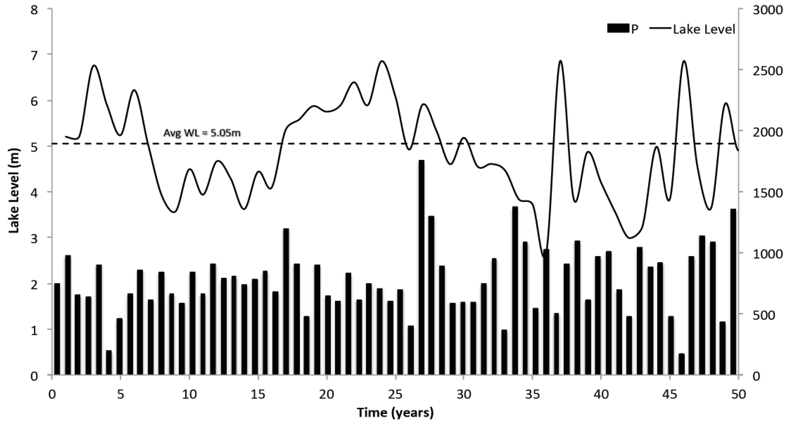
3.1. Reproducing Current Conditions and Historical Observations at Lake Babati
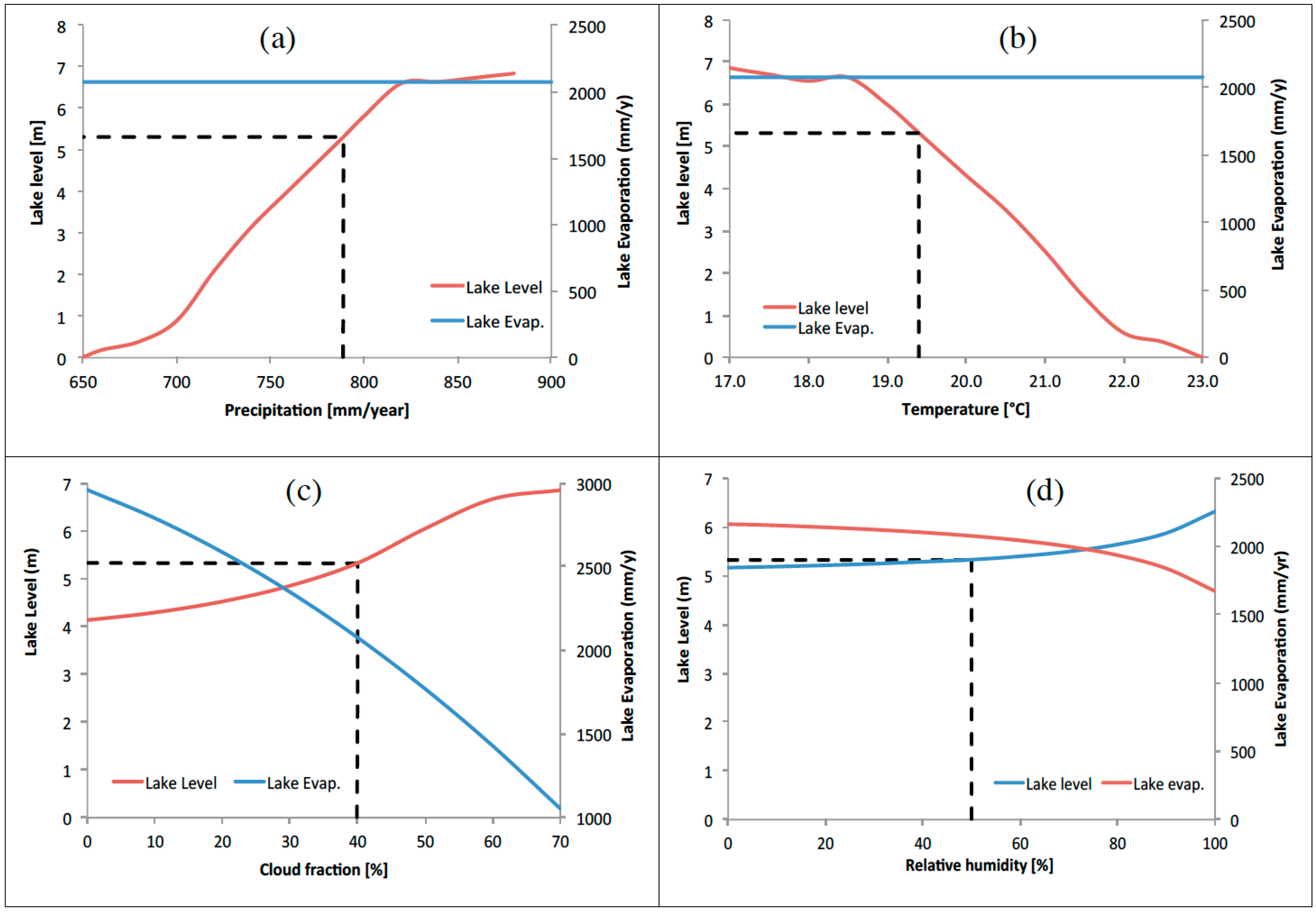
3.2. Sensitivity Analysis
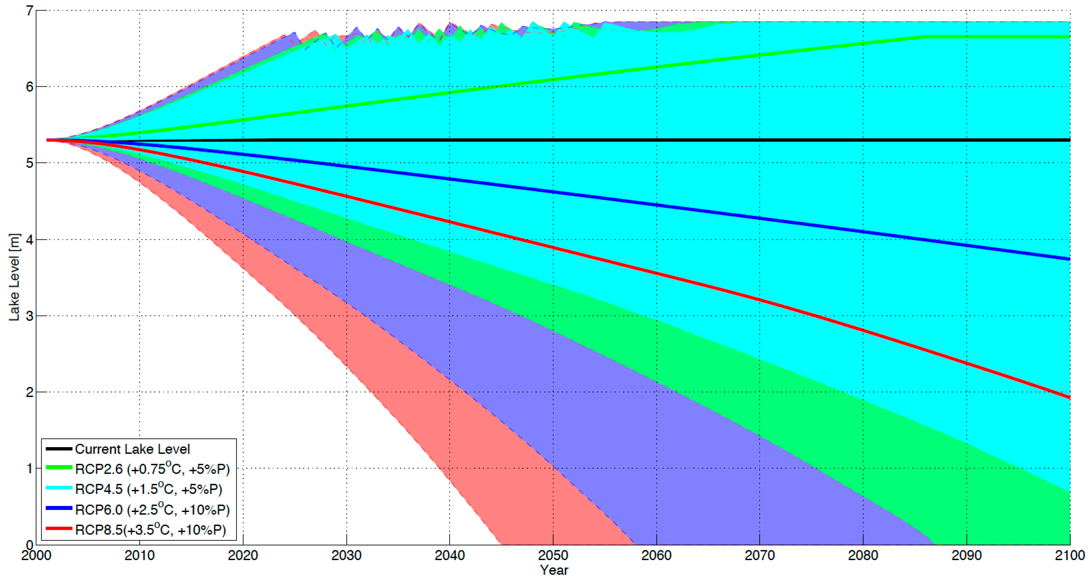
3.3. Lake Babati Response to Climate Change and Variability
4. Conclusions
Acknowledgments
Author Contributions
Conflicts of Interest
References
- Swenson, S.; Wahr, J. Monitoring the water balance of Lake Victoria, East Africa, from space. J. Hydrol. 2009, 370, 163–176. [Google Scholar] [CrossRef]
- Tate, E.; Sutcliffe, J.; Conway, D.; Farquharson, F. Water balance of Lake Victoria: Update to 2000 and climate change modelling to 2100. Hydrol. Sci. J. 2004, 49. [Google Scholar] [CrossRef]
- Yin, X.G.; Nicholson, S.E. The water balance of Lake Victoria. Hydrol. Sci. J. 1998, 43, 789–811. [Google Scholar] [CrossRef]
- Vallet-Coulomb, C.; Legesse, D.; Gasse, F.; Travi, Y.; Chernet, T. Lake evaporation estimates in tropical Africa (Lake Ziway, Ethiopia). J. Hydrol. 2001, 245, 1–18. [Google Scholar] [CrossRef]
- Kebede, S.; Travi, Y.; Alemayehu, T.; Marc, V. Water balance of Lake Tana and its sensitivity to fluctuations in rainfall, Blue Nile Basin, Ethiopia. J. Hydrol. 2006, 316, 233–247. [Google Scholar] [CrossRef]
- Deus, D.; Gloaguen, R.; Krause, P. Water balance modeling in a semi-arid environment with limited in situ data using remote sensing in Lake Manyara, East African Rift, Tanzania. Remote Sens. 2013, 5, 1651–1680. [Google Scholar] [CrossRef]
- Bergner, A.G.N.; Trauth, M.H.; Bookhagen, B. Paleoprecipitation estimates for the Lake Naivasha basin (Kenya) during the last 175 k.y. using a lake-balance model. Glob. Planet. Chang. 2003, 36, 117–136. [Google Scholar] [CrossRef]
- Borchardt, S.; Trauth, M.H. Remotely-sensed evapotranspiration estimates for an improved hydrological modeling of the early Holocene mega-lake Suguta, northern Kenya Rift. Palaeogeogr. Palaeoclimatol. Palaeoecol. 2012, 361–362, 14–20. [Google Scholar] [CrossRef]
- Legesse, D.; Vallet-Coulomb, C.; Gasse, F. Analysis of the hydrological response of a tropical terminal lake, Lake Abiyata (Main Ethiopian Rift Valley) to changes in climate and human activities. Hydrol. Process. 2004, 18, 487–504. [Google Scholar] [CrossRef]
- Koutsouris, A.J.; Destouni, G.; Jarsjö, J.; Lyon, S.W. Hydro-climatic trends and water resource management implications based on multi-scale data for the Lake Victoria region, Kenya. Environ. Res. Lett. 2010, 5. [Google Scholar] [CrossRef]
- Yin, X.; Nicholson, S.E.; Ba, M.B. On the diurnal cycle of cloudiness over Lake Victoria and its influence on evaporation from the lake. Hydrol. Sci. J. 2000, 45, 407–424. [Google Scholar] [CrossRef]
- Jarsjö, J.; Asokan, S.M.; Prieto, C.; Bring, A.; Destouni, G. Hydrological responses to climate change conditioned by historic alterations of land-use and water-use. Hydrol. Earth Syst. Sci. 2012, 16, 1335–1347. [Google Scholar] [CrossRef]
- National Bureau of Statistics (NBS). 2012 Population and Household Census. Population Distribution by Administrative Areas; National Bureau of Statistics and Office of Chief Government Statistician: Dar es Salaam and Zanzibar, Tanzania, 2013; p. 264.
- Kahurananga, J. Lake Babati, Tanzania and Its Immediate Surroundings. Part I—Baseline Information; Regional Soil Conservation Unit (SIDA): Nairobi, Kenya, 1992. [Google Scholar]
- Strömquist, L.; Johansson, D. Studies of soil erosion and sediment transport in the Mtera reservoir region, Central Tanzania. Z. Geomorphol. 1978, 29, 43–51. [Google Scholar]
- Muzuka, A.N.N.; Ryner, M.; Holmgren, K. 12,000-year, preliminary results of the stable nitrogen and carbon isotope record from the Empakai Crater lake sediments, Northern Tanzania. J. Afr. Earth Sci. 2004, 40, 293–303. [Google Scholar] [CrossRef]
- Öberg, H.; Norström, E.; Malmström Ryner, M.; Holmgren, K.; Westerberg, L.O.; Risberg, J.; Eddudóttir, S.D.; Andersen, T.J.; Muzuka, A. Environmental variability in northern Tanzania from ad 1000 to 1800, as inferred from diatoms and pollen in Lake Duluti. Palaeogeogr. Palaeoclimatol. Palaeoecol. 2013, 374, 230–241. [Google Scholar] [CrossRef]
- Ryner, M.; Holmgren, K.; Taylor, D. A record of vegetation dynamics and lake level changes from Lake Emakat, northern Tanzania, during the last c. 1200 years. J. Paleolimnol. 2008, 40, 583–601. [Google Scholar] [CrossRef]
- Ryner, M.A.; Bonnefille, R.; Holmgren, K.; Muzuka, A. Vegetation changes in Empakaai Crater, northern Tanzania, at 14,800–9300 cal·yr BP. Rev. Palaeobot. Palynol. 2006, 140, 163–174. [Google Scholar] [CrossRef]
- Strömquist, L.; Johansson, D. An Assessment of Environmental Change and Recent Lake Babati Floods, Babati District, Tanzania; LandFocus Consultants: Uppsala, Sweden, 1990. [Google Scholar]
- Sandström, K. The recent lake babati floods in semi-arid Tanzania—A response to changes in land cover? Geogr. Ann. 1995, 77 A, 35–44. [Google Scholar] [CrossRef]
- Gerdén, C.Å.; Khawange, G.M.O.; Mallya, J.M.; Mbuya, J.P.; Sanga, R.C. The Wild Lake. In The 1990 Floods in Babati, Tanzania—Rehabilitation and Prevention; Regional Soil Conservation Unit (SIDA): Nairobi, Kenya, 1992. [Google Scholar]
- Andrews, P.; Bamford, M.K.; Njau, E.F.; Leliyo, G. The ecology and biogeography of the endulen-laetoli area in northern Tanzania. In Paleontology and Geology of Laetoli: Human Evolution in Context; Harrison, T., Ed.; Springer: Dordrecht, The Netherlands, 2011; pp. 167–200. [Google Scholar]
- Koponen, J. Structures, people and production in Late Pre-Colonial Tanzania: History and structures. J. Afr. Hist. 1991, 32, 155–156. [Google Scholar]
- Strömquist, L. Environmental impact assessment of natural disasters, a case study of the recent Lake Babati floods in northern Tanzania. Geogr. Ann. Ser. A Phys. Geogr. 1992, 74, 81–91. [Google Scholar] [CrossRef]
- Newman, P.; Rönnberg, P. Changes in Land Utilization within the Last Three Decades in the Babati Area; International Rural Development Centre, Swedish University of Agricultural Sciences: Uppsala, Sweden, 1992. [Google Scholar]
- Kijazi, A.L.; Reason, C.J.C. Analysis of the 2006 floods over northern Tanzania. Int. J. Climatol. 2009, 29, 955–970. [Google Scholar] [CrossRef]
- Food and Agriculture Organization of the United Nations (FAO). New_Locclim: Local Climate Estimator Version 1.10; Environment and Natural Resources Working Paper No. 20 (CD-ROM); FAO: Rome, Italy, 2005. [Google Scholar]
- Sjödin, E. Leaking or Waterproof Organization? Babati Town and the Current Capacity to Handle Floods; Södertörn Högskola: Huddinge, Sweden, 2010. [Google Scholar]
- Yanda, P.Z.; Madulu, N.F. Water resource management and biodiversity conservation in the Eastern Rift Valley Lakes, northern Tanzania. Phys. Chem. Earth 2005, 30, 717–725. [Google Scholar] [CrossRef]
- Jarvis, A.; Reuter, H.I.; Nelson, A.; Guevara, E. Hole-Filled Seamless SRTM Data V4. International Center for Tropical Agriculture (CIAT). 2008. Available online: http://srtm.csi.cgiar.org (accessed on 17 September 2015).
- Hutchinson, M.F. A new procedure for gridding elevation and stream line data with automatic removal of spurious pits. J. Hydrol. 1989, 106, 211–232. [Google Scholar] [CrossRef]
- Brutsaert, W. Evaporation into the Atmosphere: Theory, History, and Applications; Reidel: Dordrecht, The Netherlands, 1982; p. 299. [Google Scholar]
- Morton, F.I. Practical estimates of lake evaporation. J. Clim. Appl. Meteorol. 1986, 25, 371–387. [Google Scholar] [CrossRef]
- Penman, H.L. Natural evaporation from open water, bare soil and grass. Proc. R. Soc. Lond. Ser. A Math. Phys. Sci. 1948, 193, 120–145. [Google Scholar] [CrossRef]
- Singh, V.P.; Xu, C.Y. Evaluation and generalization of 13 mass-transfer equations for determining free water evaporation. Hydrol. Process. 1997, 11, 311–323. [Google Scholar] [CrossRef]
- Kummu, M.; Tes, S.; Yin, S.; Adamson, P.; Józsa, J.; Koponen, J.; Richey, J.; Sarkkula, J. Water balance analysis for the tonle sap lake-floodplain system. Hydrol. Process. 2014, 28, 1722–1733. [Google Scholar] [CrossRef]
- Kutzbach, J.E. Estimates of past climate at Paleolake Chad, North Africa, based on a hydrological and energy-balance model. Quat. Res. 1980, 14, 210–223. [Google Scholar] [CrossRef]
- Lenters, J.D.; Kratz, T.K.; Bowser, C.J. Effects of climate variability on lake evaporation: Results from a long-term energy budget study of Sparkling Lake, northern Wisconsin (USA). J. Hydrol. 2005, 308, 168–195. [Google Scholar] [CrossRef]
- Rosenberry, D.O.; Sturrock, A.M.; Winter, T.C. Evaluation of the energy budget method of determining evaporation at Williams Lake, Minnesota, using alternative instrumentation and study approaches. Water Resour. Res. 1993, 29, 2473–2483. [Google Scholar] [CrossRef]
- Winter, T.C. Uncertainties in estimating the water balance of lakes. JAWRA J. Am. Water Resour. Assoc. 1981, 17, 82–115. [Google Scholar] [CrossRef]
- Hastenrath, S.; Kutzbach, J.E. Paleoclimatic estimates from water and energy budgets of East African lakes. Quat. Res. 1983, 19, 141–153. [Google Scholar] [CrossRef]
- Black, J.N.; Bonython, C.W.; Prescott, J.A. Solar radiation and the duration of sunshine. Q. J. R. Meteorol. Soc. 1954, 80, 231–235. [Google Scholar] [CrossRef]
- Budyko, M.I. Climate and Life; Academic Press: New York, NY, USA, 1974. [Google Scholar]
- Langbein, W.B. Annual runoff in the United States. Geol. Surv. Circ. 1949, 52, 14. [Google Scholar]
- Turc, L. The water balance of soils. Relation between precipitation, evaporation and flow. Ann. Agron. 1954, 5, 491–569. [Google Scholar]
- Jarsjö, J.; Shibuo, Y.; Destouni, G. Spatial distribution of unmonitored inland water discharges to the sea. J. Hydrol. 2008, 348, 59–72. [Google Scholar] [CrossRef]
- SWECO International, Water Geosciences Consulting, Council for Geosciences and Water Resources Consultants. SADC Hydrogeological Map and Atlas; Water Division—SADC Infrastructure and Services Directorate: Gaborone, Botswana, 2010. [Google Scholar]
- MacDonald, A.M.; Bonsor, H.C.; Dochartaigh, B.É.Ó.; Taylor, R.G. Quantitative maps of groundwater resources in Africa. Environ. Res. Lett. 2012, 7, 260–261. [Google Scholar] [CrossRef]
- Weight, W.D.; Zaluski, M.; Sonderegger, J.L. Manual of Applied Field Hydrogeology (Elektronisk Resurs); McGraw-Hill: New York, NY, USA, 2001. [Google Scholar]
- Nicholson, S.; Yin, X. Rainfall conditions in equatorial East Africa during the nineteenth century as inferred from the record of Lake Victoria. Clim. Chang. 2001, 48, 387–398. [Google Scholar] [CrossRef]
- Asokan, S.M.; Jarsjö, J.; Destouni, G. Vapor flux by evapotranspiration: Effects of changes in climate, land use, and water use. J. Geophys. Res. 2010, 115, 9–12. [Google Scholar] [CrossRef]
- Törnqvist, R.; Jarsjö, J.; Pietroń, J.; Bring, A.; Rogberg, P.; Asokan, S.M.; Destouni, G. Evolution of the hydro-climate system in the Lake Baikal basin. J. Hydrol. 2014, 519, 1953–1962. [Google Scholar] [CrossRef]
- Törnqvist, R.; Jarsjö, J. Water savings through improved irrigation techniques: Basin-scale quantification in semi-arid environments. Water Resour. Manag. 2012, 26, 949–962. [Google Scholar] [CrossRef]
- Raes, D.; Mallants, D.; Song, Z. Rainbow—A software package for analysing hydrologic data. In Hydraulic Engineering Software VI; Blain, W.R., Ed.; Computational Mechanics Publications: Southampton, UK; Boston, MA, USA, 1996; pp. 525–534. [Google Scholar]
- The Royal Netherlands Meteorological Institute (KNMI). Climate Explorer—Climate Change Atlas. De Bilt, The Netherlands. 2015. Available online: https://climexp.knmi.nl (accessed on 17 September 2015).
- Intergovernmental Panel on Climate Change (IPCC). Climate Change 2013: The Physical Science Basis. Contribution of Working Group I to the Fifth Assessment Report of the Intergovernmental Panel on Climate Change; Cambridge University Press: Cambridge, UK; New York, NY, USA, 2013; p. 1535. [Google Scholar]
- Dühnforth, M.; Bergner, A.N.; Trauth, M. Early holocene water budget of the Nakuru-Elmenteita basin, central Kenya Rift. J. Paleolimnol. 2006, 36, 281–294. [Google Scholar] [CrossRef]
- Odada, E.; Olago, D.; Bugenyi, F.; Kulindwa, K.; Karimumuryango, J.; West, K.; Ntiba, M.; Wandiga, S.; Aloo-Obudho, P.; Achola, P. Environmental assessment of the East African Rift Valley Lakes. Aquat. Sci. 2003, 65, 254–271. [Google Scholar] [CrossRef]
- Olaka, L.A.; Odada, E.O.; Trauth, M.H.; Olago, D.O. The sensitivity of East African Rift Lakes to climate fluctuations. J. Paleolimnol. 2010, 44, 629–644. [Google Scholar] [CrossRef]
- Ayenew, T.; Becht, R. Comparative assessment of the water balance and hydrology of selected Ethiopian and Kenyan Rift Lakes. Lakes Reserv. Res. Manag. 2008, 13, 181–196. [Google Scholar] [CrossRef]
- United Nations Environment Programme (UNEP). World atlas of Desertification; UNEP: London, UK, 1992. [Google Scholar]
- Shanahan, T.M.; Overpeck, J.T.; Sharp, W.E.; Scholz, C.A.; Arko, J.A. Simulating the response of a closed-basin lake to recent climate changes in tropical West Africa (Lake Bosumtwi, Ghana). Hydrol. Process. 2007, 21, 1678–1691. [Google Scholar] [CrossRef]
- Lyon, S.W.; Koutsouris, A.; Scheibler, F.; Jarsjö, J.; Mbanguka, R.; Tumbo, M.; Robert, K.K.; Sharma, A.N.; van der Velde, Y. Interpreting characteristic drainage timescale variability across Kilombero Valley, Tanzania. Hydrol. Process. 2015, 29, 1912–1924. [Google Scholar] [CrossRef]
- Tessema, S.; Lyon, S.; Setegn, S.; Mörtberg, U. Effects of different retention parameter estimation methods on the prediction of surface runoff using the SCS curve number method. Water Resour. Manag. 2014, 28, 3241–3254. [Google Scholar] [CrossRef]


| Model Input | Estimated Current Value | |
|---|---|---|
| Precipitation (mm/year) | 789.0 | |
| Temperature (°C) | 19.4 | |
| Relative Humidity (%) | 50.0 | |
| Lake surface area (km2) | 6.9 | |
| GW reservoir area (km2) | 48.1 | |
| Total catchment area (km2) | 355.0 | |
| Groundwater conductivity (m/day) | 50.0 | |
| Porosity (%) | 40.0 | |
| Calibrated parameters | Physical range | Optimum value |
| Cloud Cover (C) (%) | 0.3–0.5 | 0.40 |
| Calibration factor for ET (Xc) | 0.7–1.2 | 1.15 |
| Climate Variable | RCP2.6 | RCP4.5 | RCP6.0 | RCP8.5 |
|---|---|---|---|---|
| Temperature Change (°C) | +0.75 (0.6) | +2 (0.1) | +2.5 (0.4) | +3.5 (0.5) |
| Precipitation Change (%) | +5 (21) | +10 (16) | +10 (27) | +10 (33) |
| Component/Term | Value |
|---|---|
| Lake depth (m) | 5.32 |
| Lake volume (m3) | 1.391 × 10⁷ |
| Precipitation over the lake (m3/year) | 5.331 × 10⁶ |
| Precipitation over ground (m3/year) | 2.679 × 10⁸ |
| Lake Evaporation (m3/year) | 1.437 × 10⁷ |
| Actual ET over ground (m3/year) | 2.552 × 10⁸ |
| Groundwater Leakage (m3/year) | 3.671 × 10⁶ |
| Lake overflow volume (m3/year) | 0 |
| Discrepancy (as % of Lake Volume) | <1% |
| Net lake evaporation depth (mm/year) | 1286 |
| Lake inflow factor (-) | 0.7 |
| Lake Level Change | Temperature (°C) | Precipitation (mm/Year) | Cloud Cover (%) | Relative Humidity (%) |
|---|---|---|---|---|
| Current to Overflow | −2.4 | +90 | +30 | did not occur |
| Current to Dry-out | +3.6 | −140 | did not occur | did not occur |
| Dry-out to overflow (absolute) | 6 | 230 | n/a | n/a |
© 2016 by the authors; licensee MDPI, Basel, Switzerland. This article is an open access article distributed under the terms and conditions of the Creative Commons Attribution (CC-BY) license (http://creativecommons.org/licenses/by/4.0/).
Share and Cite
Mbanguka, R.P.; Lyon, S.W.; Holmgren, K.; Girons Lopez, M.; Jarsjö, J. Water Balance and Level Change of Lake Babati, Tanzania: Sensitivity to Hydroclimatic Forcings. Water 2016, 8, 572. https://doi.org/10.3390/w8120572
Mbanguka RP, Lyon SW, Holmgren K, Girons Lopez M, Jarsjö J. Water Balance and Level Change of Lake Babati, Tanzania: Sensitivity to Hydroclimatic Forcings. Water. 2016; 8(12):572. https://doi.org/10.3390/w8120572
Chicago/Turabian StyleMbanguka, René P., Steve W. Lyon, Karin Holmgren, Marc Girons Lopez, and Jerker Jarsjö. 2016. "Water Balance and Level Change of Lake Babati, Tanzania: Sensitivity to Hydroclimatic Forcings" Water 8, no. 12: 572. https://doi.org/10.3390/w8120572
APA StyleMbanguka, R. P., Lyon, S. W., Holmgren, K., Girons Lopez, M., & Jarsjö, J. (2016). Water Balance and Level Change of Lake Babati, Tanzania: Sensitivity to Hydroclimatic Forcings. Water, 8(12), 572. https://doi.org/10.3390/w8120572