On the Simulation of Floods in a Narrow Bending Valley: The Malpasset Dam Break Case Study

Abstract

In this paper, we investigate the performance of three-dimensional (3D) hydraulic modeling when dealing with river sinuosity and meander bends. In river bends, the flow is dominated by a secondary current, which has a key role on the flow redistribution. The secondary flow induces transverse components of the bed shear stress and increases the velocity in outward direction, thus generating local erosion and riverbed modifications. When in river bends, the 3D processes prevail, and a 3D computational fluid dynamics (CFD) model is required to correctly predict the flow structure. An accurate description of the different hydrodynamic processes in mildly and sharply curved bends find a relevant application in meanders migration modeling. The mechanisms that drive the velocity redistribution in meandering channels depend on the river’s roughness, the flow depth (H), the radius curvature (R), the width (B) and the bathymetric variations. Here, the hydro-geomorphic characterization of sharp and mild meanders is performed by means of the ratios R/B, B/H, and R/H, and of the sinuosity index. As a case study, we selected the Malpasset dam break on the Reyran River Valley (FR), as it is perfectly suited for investigating performances and issues of a 3D model in simulating the inundation dynamics in a river channel with a varying curvature radius.

1. Introduction

The detailed study of hydraulic processes in sharply-curved bends is of practical relevance [1] as the water flow and sediment transport generate local erosion resulting in bed changing and impacting infrastructures. Moreover, the morphological variations of cross-sections have a relevant role in supporting flood propagation and inundation modeling [2,3,4].

The flow field in river bends is highly three-dimensional [5,6], being characterized by secondary flows that cause high bank shear stress and erosion of the outer part of the bend. Indeed, cut-off events, representing the driving mechanism of long-term and large-scale meander morphologic dynamics, typically occur in sharply-curved bends [7]. Meandering rivers represent fluvial geometric settings where three-dimensional (3D) models have a high performance because of the complex characterization of the flow [5].

This paper deals with the investigation of the hydraulic processes governing the velocity redistribution and water surface elevation in sharply-curved open-channel bends by means of a detailed 3D numerical simulation. The selected case study is the Malpasset dam break [8] characterized by a significant amount of field and laboratory data [9,10,11]. Many authors dealt with the issue of modeling the propagation of the flood waves caused by the failure of dams [12,13] to define the event that led to the dam breaching [14] and the effects of the flood downstream [15]. The propagation of the flood wave generated by the Malpasset dam break have already been studied through one- and two-dimensional models [9,16,17,18]. In this paper, the breaching of the Malpasset dam is used to numerically investigate the flood wave propagation in a bending channel using a 3D model. Since the mechanisms that drive the velocity redistribution in meandering channels depend on the river’s roughness, on the flow depth (H), radius curvature (R), width (B) and bathymetric variations, the hydro-geomorphic characterization of the meanders is performed by means of the ratios R/B, B/H, and R/H and of the sinuosity index (SI). In the following, a brief overview on computational fluid dynamics (CFD) models and on the geomorphological representation of river channel is provided.

1.1. Computational Fluid Dynamics Models in the Framework of Curved Channels

The increasing computational power and efficiency together with the higher availability and resolution of remotely sensed topographic and land use data are paving the way for the use of complex and detailed numerical models to simulate fluvial hydraulic processes. In recent years, hydraulic modeling applications have passed from coarse scale (10–100 m) one-dimensional models to 3D flexible mesh hydrodynamics simulations. At present, 3D CFD have demonstrated to provide stable and accurate modeling capabilities without any further need of the simplified assumptions that were originally needed by 1D schemes [19]. Performances of CFD now have a significant track record [20,21,22,23,24,25] with several tests found in the literature specifically with regard to spatially rapidly varied flow conditions with vertical component [26,27,28]. CFD models simulate effectively fluvial settings characterized by high hydrodynamic complexity [29,30]. For instance, Baranya et al. [31] used CFD for simulating confluences of two medium-sized Hungarian rivers through a 3D Reynolds-averaged Navier–Stokes (RANS) model.

The simulation of floods in meandering channel using CFD models is of actual scientific interest [21,32]. In fact, given the complexity of the flow field in meandering bends, 3D CFD models are required to correctly predict the secondary flows [22]. Several research works dealt with the need to model the distribution of the main flow, the magnitude of the secondary flow, the direction of the bed shear stress and the curvature induced additional energy losses in high curvature bends (e.g., Blanckaert and de Vriend [23]). Riley and Rhoads [33] investigated the flow structure where complex natural and artificial singularities impact the flow (i.e., at confluences and bifurcations). Eddy-resolving numerical models are used to investigate the flow processes, which include secondary flow, large scale coherent turbulence structures, shear layers and flow separation at the convex inner bank [34]. Many authors studied the three-dimensional processes in curved open channels through the eddy-resolving methods to solve the large scales of the turbulent motion [35,36]. Koken et al. [37] and van Balen et al. [38] investigated sharply curved open channel flows with a flat-bed through eddy-resolving numerical simulations. Since the irregularity of flood flow patterns in sharp bends characterizes most river reaches, the range of validity of the simplified assumptions of 1D and 2D models is a relevant issue, as investigated by Zeng et al. [39] and Blanckaert and de Vriend [40], who review the existing numerical models for meandering rivers with particular emphasis on the effect of secondary flows.

1.2. The Geomorphologic Characterization of a River Channel

As mild and sharp river bends are characterized by substantially different hydrodynamic processes, it is important to properly describe the velocity field in these two scenarios. Indeed, when dealing with mildly curved bends, the velocity redistribution is negligible, while it becomes a dominant process in sharply curved bends [41]. This is a relevant finding especially when dealing with meander models. In fact, the hydrodynamic component plays a relevant role in describing the flow field and the shear stresses close to both the riverbed and the bank, as it is the driver of the migrating bars and banks, respectively. Fluvial channel migration is also caused by local flow structure and dynamics, with particular regard to flow deflection due to material accumulated on the inside bend. The fluvial buffer morphologic evolution is governed by these factors, as well as the potential bank instability in flooding conditions, given the development of high velocities and turbulence kinetic energy near the bank toe of sharp bends.

This paper presents a fully 3D model of the flow field in a river channel characterized by different bending, ranging from mild to sharp. As found by [40], the mechanisms that drive the velocity redistribution in meandering channels depend on the river’s roughness, flow depth (H), radius curvature (R), width (B) and bathymetric variations. As a matter of fact, the identification of the curvature type (i.e., weak, moderate, and strong) is based on the ratios R/H and R/B or on the turbulent Dean number [23,42], while the ratio B/H distinguishes shallow natural rivers from narrow laboratory water channels [40].

Many authors dealt with meandering channels using the aforementioned ratios. For instance, Engel and Rhoads [43] evaluated the meanders evolution throughout the time with several campaigns on a specific river, characterizing the bends with the ratios R/B and H/B. Ottevanger et al. [41] examined a wide range of topographic configurations (e.g., mildly to sharply curved bends, narrow to shallow bends) confirming that the topography drives the flow redistribution and, specifically, the secondary flow.

The close relationship between the geomorphological characteristics of the downstream valley and the generation of the secondary flow is here investigated by means of the R/B, B/H and R/H ratios that parameterize the meander hydrodynamics together with the curvature radius, the top width channel and the flow depth.

Moreover, in this paper, the sinuosity of the river is also considered as an important geomorphic parameter and is expressed by the sinuosity index (SI), which measures the deviation of a line from the shortest path [44].

The indexes SI, R/B, B/H and R/H are calculated using a geographic information system (GIS) analysis to quantitatively characterize the river curvature type, distinguishing sharp and mild bends from rectilinear reaches.

The aim of this work is to assess potential limitations and range of application of fully 3D CFD simulations for hydraulic flows in complex geometries. Specifically, the flow characteristics in a narrow bending valley after the sudden collapse of a dam are analyzed.

The paper is organized as follows. In the following section, we describe the test case study, and pre-event condition is provided by a historical 1:20,000 map. Then, the theoretical and numerical specifications of the 3D numerical model are presented. We compare water depth and arrival time obtained through the 3D numerical model with fields and laboratory data. The geometric and morphodynamic indexes are analyzed to evaluate the relation between river channel curvature and hydraulic model performance.

2. Test Site: The Malpasset Dam in the Reyran River Valley (FR)

The Malpasset dam was an arch dam built in the period from 1952 to 1954 in the Reyran River Valley, about 12 km upstream of the Frejus, located in the Cote d’Azur area, southern France. It was a doubly curved arch dam with equal angle and variable radius, originally built to supply water to the region and for flood risk management to reduce potential inundation risk in the Reyran River. Downstream of the dam, the valley has two narrow bends that widen before narrowing again. A map of the region with terrain elevation is shown in Figure 1.

In 1959, the dam failed explosively and gave rise to a 40 m high flooding wave. Such a wave reached the Frejus gulf about 21 min after the dam break. The release of about 50 millions m³ of water in the 12 km long river valley down to the town of Frejus killed 421 people and produced close to $70 million in damage [45]. Only a small portion of the arch of the dam still remains in its original position. Several investigations were conducted in the aftermath to understand the cause of the failure. The reports state that the involved engineers did not correctly evaluate the exceptional rainfall that occurred. Moreover, the lack of accurate geological survey information impacted a safe dam design.

Significant field data are available for the Malpasset dam break test case. In fact, the flood wave arrival times are available, as the three hydroelectric plants along the Reyran River were turned off by the flood impact. The maximum water depth values are available because they were registered by the police after the flood event. Moreover, the National Hydraulic and Environment Laboratory of Electricité de France (EDF) built a 1:400 physical scale model of the case study [8], simulating the flood wave and measuring both water depth and arrival time values in specific points. These field and laboratory data are here used to verify the performance of the 3D hydraulic simulation. Specifically, the focus is drawn on the efficiency and the accuracy of such detailed model to simulate unsteady complex flood flows within real domains characterized by a very complex geometry.

3. Methodology: The Three-Dimensional CFD Model

The three-dimensional simulation of free-surface hydraulic flows is here performed through the Volume of Fluid (VOF) method [47,48,49] implementing a numerical solution for the incompressible flow of two immiscible fluids (i.e., air and water), tracking the interface between them [50]. According to this methodology, a single set of mass and momentum conservation equations for incompressible flows is solved for both phases (i.e., air and water). The interface between water and air is tracked through the water volume fraction γ. Given an infinitesimal control volume within the domain, the value of γ is null if the volume is entirely occupied by air, while it equals 1 either when the volume is entirely occupied by water or when the volume contains the interface between water and air.

The resulting mathematical model consists of the following mass and momentum conservation equations (i.e., Navier–Stokes equations):

$$\nabla \cdot u=0$$

(1)

$$\frac{D\left(\mathsf{\rho }u\right)}{Dt}-\nabla \cdot \left[\left(\mathsf{\mu }+{\mathsf{\mu }}_t\right)S\right]=-\nabla p+\mathsf{\rho }g$$

(2)

and the transport equation for the fraction fill function:

$$\frac{D\mathsf{\gamma }}{Dt}+\nabla \cdot \left[w_r\mathsf{\gamma }\left(1-\mathsf{\gamma }\right)\right]=0$$

(3)

where u is the velocity vector, p is the pressure, ρ is the fluid mass density, μ is the dynamic viscosity, and w_r is the relative velocity between the two phases. The term $\nabla \cdot \left[\left(\mu +{\mu }_t\right)S\right]$, where S is the strain rate tensor and μ_t is the turbulent eddy viscosity, derives from the application of the k-ε eddy viscosity turbulence model [51]. Such a model represents the turbulence problem through two variables, the turbulent kinetic energy, k, and the turbulent dissipation rate, ε. The turbulent eddy viscosity is then calculated as

$${\mathsf{\mu }}_t=\frac{c_{\mathsf{\mu }}{f}_{\mathsf{\mu }}\mathsf{\rho }{k}^2}{\mathsf{\epsilon }}$$

(4)

where c_μ is a constant parameter and f_μ is a damping function. The values of k and ε are then governed by advection diffusion equations, as explained in detail in [52].

It is interesting to note that, although the flow is assumed to be incompressible, the fluid mass density varies in time as the phase fractions of the infinitesimal volumes containing the free surface change in time:

$$\rho \left(t\right)=\gamma {\rho }_w+\left(1-\gamma \right){\rho }_a$$

(5)

where ${\rho }_w$ and ${\rho }_a$ are the constant fluid mass densities of water and air, respectively.

Concerning the free surface tracking, the transport equation (Equation (3)) contains an additional convective term, which is used to reduce the diffusion of the interface [53] providing a sharper interface resolution.

The numerical resolution of the system of Equations (1)–(4) is performed through the finite volume technique in the framework of the open source CFD package OpenFOAM [54]. The spatial domain is discretized through the Gauss linear procedure and the Pressure Implicit with Split Operators (PISO) algorithm is the pressure–velocity calculation procedure used to solve the Navier–Stokes equations [55]. Furthermore, we employ the Multidimensional Universal Limiter with Explicit Solution (MULES) to solve the Equation (3). The employed three-dimensional model has been extensively validated in previous studies against analytical and laboratory data [56,57,58].

In the following, the 3D mesh generation to build the hydraulic 3D model is presented.

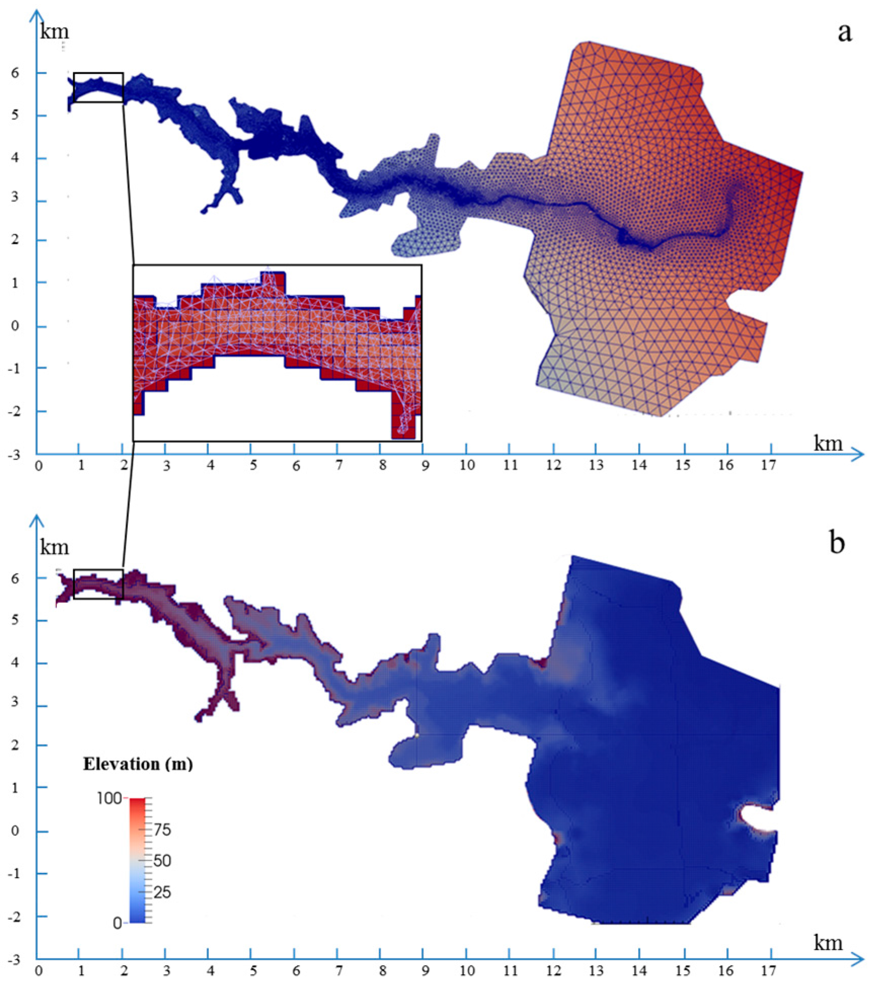
Domain Geometry: Digital Terrain Model

The creation of the computational mesh is performed through the following steps: (a) construction of the terrain model from elevation points; (b) creation of the computational domain limits and of a coarse mesh; and (c) mesh–terrain surface intersection and local mesh refinement and snapping.

The Reyran River valley morphology changed significantly because of the flood wave originated by the dam collapse. The computational mesh in pre-event conditions has been constructed by using the information available in a historical 1:20,000 map, dated 1931, provided by the Institut Geographique National (IGN) and later digitized by EDF [9]. The bounding box of the domain of interest is 17,500 m wide and 10,000 m high. The topographic elevation ranges from 0 m to 100 m above sea level, the latter being the upstream boundary condition corresponding to the initial reservoir water level. The digital representation of the domain is developed using 13,541 points of known coordinates. The valley geometry, provided by EDF [46,59], is a non-structured grid of 13,000 points reported in Figure 1.

The characteristics of the final mesh (Figure 2) are reported in

Table 1. Characteristics of the final mesh: number of points, number of total and internal faces, number of cells and number of boundary patches.

Points	Faces	Internal Faces	Cells	Boundary Patches
2,287,929	6,693,676	6,524,876	2,203,092	7

. No-slip boundary conditions are imposed at the walls and free slip at the atmosphere boundary, located for the present simulations at 140 m.a.s.l. Following the information provided by EDF, and consistently with the reference system of the map, the dam is considered as a straight line between the points of coordinates (4701, 4143) and (4655, 4392). As initial boundary condition, the water level upstream of the dam is set to 100 m and the rest of the valley is assumed to be in dry conditions, although a certain discharge was flowing out of the dam at burst time.

4. Results and Discussion

The 3D model results are compared with observed data and with results obtained using a scale model built in the National Hydraulic and Environment Laboratory of EDF in 1964 [8,46]. Results are analyzed in relation to the geomorphological characteristics of the main channel to understand the relationship between the narrow bending meanders of the river and the simulation performances in modeling the irregular rapidly varying flood wave.

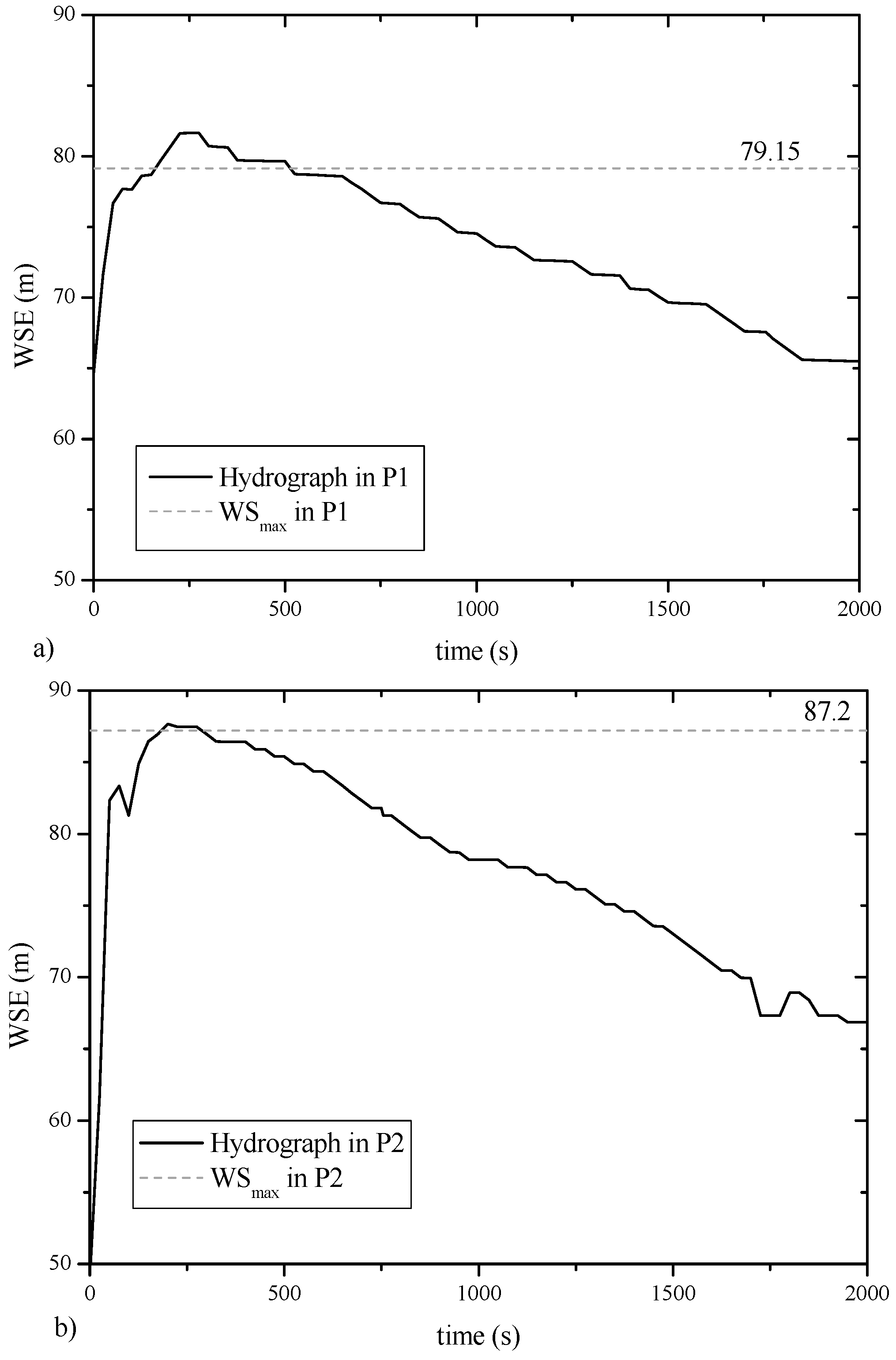
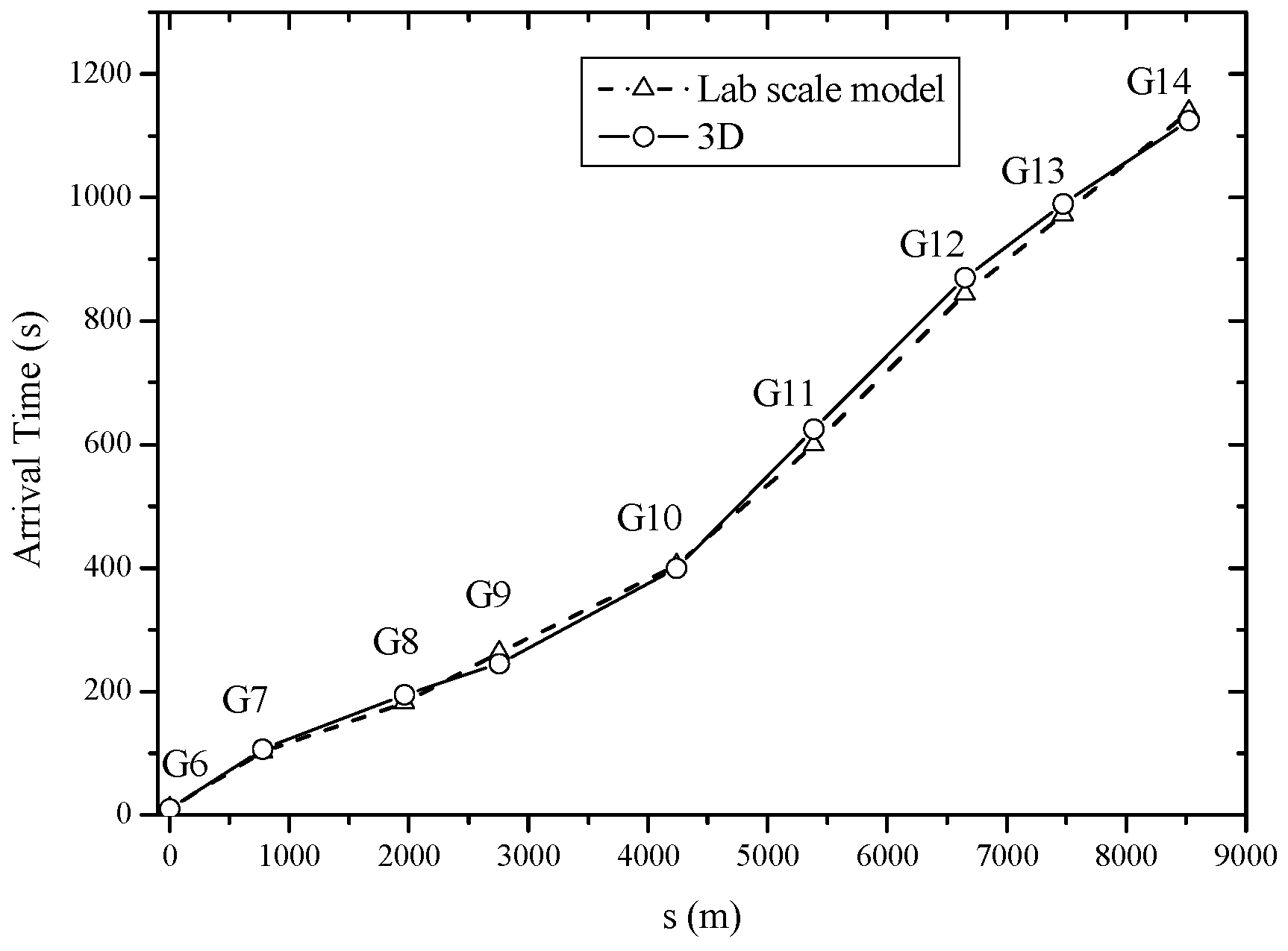
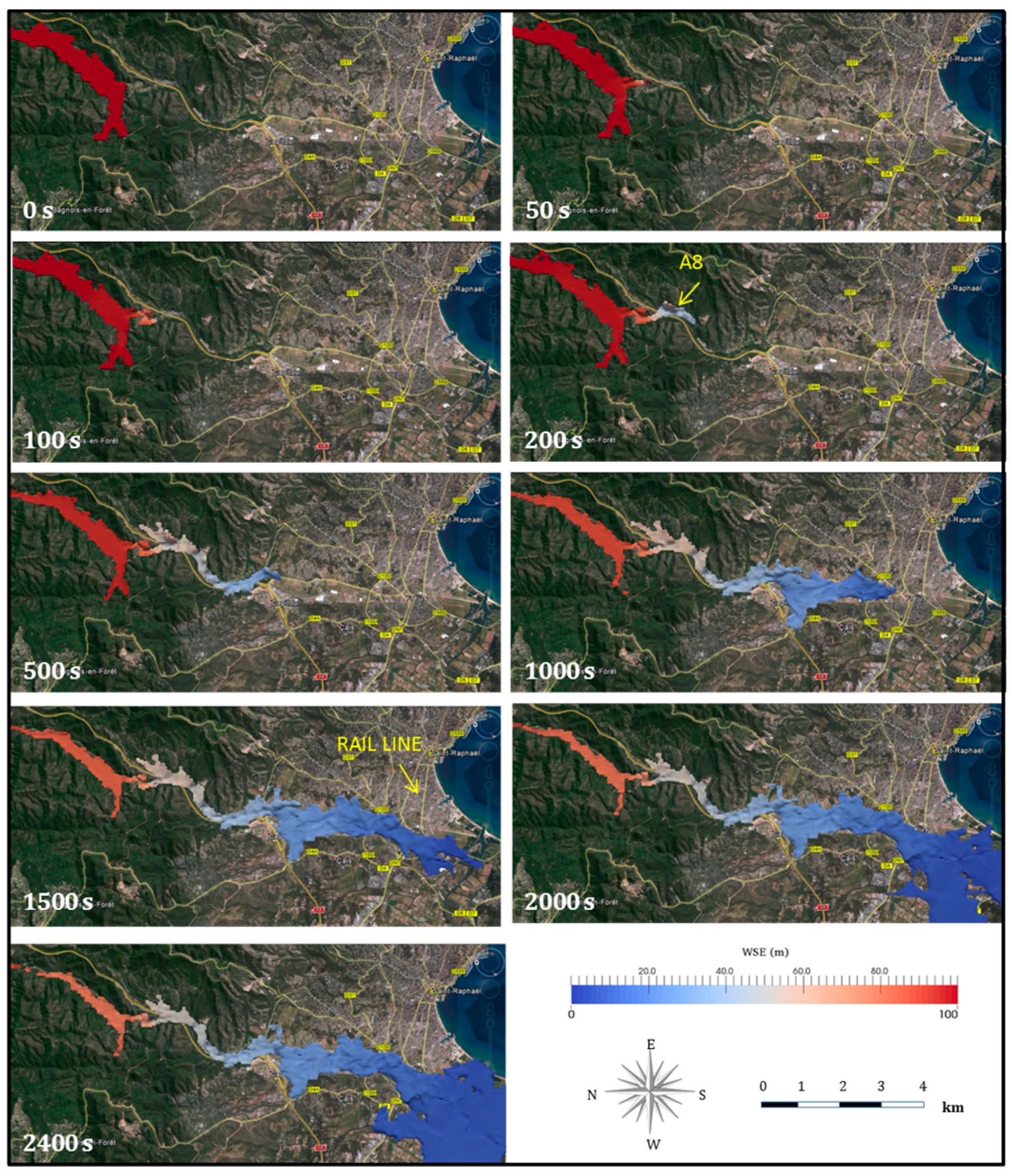
4.1. Numerical Simulation: Comparison with Field and Laboratory Data

The flow is initialized with both phases at rest and the pressure field in accordance to the hydrostatic profile. A transient 3D fluid dynamics simulation, starting from the collapse of the dam, is performed in the whole domain depicted in Figure 1.

The propagation time of the wave front is assumed to be synchronous with the Shutdown Times (STs) of the Electrical Transformers (ETs) of three hydroelectric plants placed along the river, downstream of the barrage, hereafter indicated as A, B and C (Figure 1). The wave arrival time (AT_obs) can be assumed to be the ST of the transformer A, which was located just downstream of the dam. For the other two transformers, B and C, the ST can be assumed to be between the wave arrival time and the time of peak water level.

Table 2. Comparison of the arrival times at the three Electrical Transformers (ETs), the observed wave arrival time (AT_obs), the distance between each transformer and the following one (Δs), the mean velocity of the flood wave between transformers sections (v), the mean value of flow arrival times at each transformer computed through 3D model (AT_3D), and the mean velocity of the flood wave simulated by the 3D model (v_3D).

ET	X (m)	Y (m)	Δs (m)	ATobs (s)	AT3D (s)	v (m/s)	v3D (m/s)
A	5500	4400	0	100	100	-	-
B	11,900	3250	6502	1240	1175	5.70	6.05
C	13,000	2700	1230	1420	1425	6.83	4.92

summarizes the available data of the flood wave arrival times (AT_obs), including the position of the three ETs. The distance from each ET and the following one on the centerline is named Δs; the flood velocity (v) is calculated as the ratio between Δs and ΔT, ΔT being the interarrival time of the flood wave at two ETs.

The flood wave arrival time at each transformer obtained with the 3D model is compared with the observations (Table 2). Concerning the analysis of the flood wave ATs at the three ETs, it is interesting to note that the 3D simulation results match the surveyed data, especially at ETs A and C, while, at ET B, the error between observed and simulated AT also affects the flood wave velocity estimation.

The maximum water levels reached by the dam break flood was observed and recorded by local police in nearly 100 points along the right and the left side of the Reyran River Valley [59]. The uncertainty of such water elevation field data is not available. The validation of the 3D numerical simulation is performed in 17 points, hereafter denoted as P1–P17. The position of these points is indicated in Figure 1, while their coordinates are reported in

Table 3. Maximum water levels at the gauge points P1–P17: data surveyed by the local police after the dam break (WS_obs), and 3D model results (WS-3D).

Points	X (m)	Y (m)	Bank -	WSobs (m)	WS-3D (m)
P1	4913.1	4244.0	Right	79.15	81.65
P2	5159.7	4369.6	Left	87.2	87.57
P3	5790.6	4177.7	Right	54.9	53.91
P4	5886.5	4503.9	Left	64.7	63.85
P5	6763.0	3429.6	Right	51.1	47.21
P6	6929.9	3591.8	Left	43.75	45.08
P7	7326.0	2948.7	Right	44.35	44.00
P8	7451	3232.1	Left	38.6	37.8
P9	8735.9	3264.6	Right	31.9	31.57
P10	8628.6	3604.6	Left	40.75	37.21
P11	9761.1	3480.3	Left	24.15	23.3
P12	9832.9	2414.7	Right	24.9	26
P13	10,957.2	2651.9	Right	17.25	16.9
P14	11,115.7	3800.7	Left	20.7	21.2
P15	11,689	2592.3	Right	18.6	18.67
P16	11,626	3406.8	Left	17.25	19
P17	12,333.7	2269.7	Right	14	15

.

The maximum water levels predicted by the 3D model (WS-3D) at gauge points P1–P17 is compared with the in situ surveys (WS_obs; Table 3). The difference between 3D model results and the field data measured by the local police after the dam failure is always less than 5%, except for points P5, P10, P16 and P17, where it ranges from 7% to 10%.

If we refer to point P2, the maximum water stage elevation computed with the 3D model (WS-3D) is very close to the one measured by the police after the event (WS_obs). Indeed, the difference between observed and simulated value equals 0.37 m.

Figure 3 shows the flood hydrograph predicted by the 3D model at points P1 and P2. It represents the water surface elevation as a function of time. It is interesting to note that the maximum value predicted by the model is very close to that surveyed by the police after the dam break.

A non-distorted 1:400 scale model of the Malpasset dam and the related river valley was built in the National Hydraulic and Environment Laboratory of EDF in 1964 [8,46]. The maximum free surface elevation and the wave arrival time values were measured at fourteen points. Five of these gauge points were located in the dam reservoir.

Table 4. Arrival time (AT) and water surface (WS) results from the in-scale model (AT_lab, WS_lab) [8,46] and from the present 3D computational results (AT_3D, WS-3D). The errors between laboratory data and 3D model results are AT_err, WS_err.

Points	X (m)	Y (m)	ATlab (s)	AT3D (s)	WSlab (m)	WS-3D (m)
G6	4947.4	4289.7	10.2	10	84.2	87.5
G7	5717.3	4407.6	102	107	49.1	53.7
G8	6775.1	3869.2	182	195	54	52.1
G9	7128.2	3162	263	245	40.2	44.2
G10	8585.3	3443.1	404	400	34.9	35.29
G11	9675	3085.9	600	625	27.4	26.1
G12	10,939.1	3044.8	845	870	21.5	21.4
G13	11,724.4	2810.4	972	990	16.1	17.4
G14	12,723.7	2485.1	1139	1125	12.9	13.4

summarizes the information regarding the physical model, including the location of the gauges and the corresponding experimental measurements of wave arrival times (AT_lab) and water surface levels (WS_lab).

The 3D numerical model results are compared with experimental data obtained with the scale model in fourteen points, named Gi and indicated in Figure 1. In absence of further observed water surface elevation, the values obtained in the laboratory model are considered as truth for the comparison. The water surface elevation and the wave arrival times in points G6–G14 obtained through the proposed three-dimensional model (WS-3D) are compared with laboratory measurements in Table 4 and Figure 4.

The potentiality of a 3D analysis is the possibility of investigating details that could not be caught with other means. Figure 5 shows the wave propagation in the Reyran valley at different time instants after the collapse of the dam and clearly shows the opportunity of obtaining a detailed picture of the flood event evolution. At 200 s after the dam collapse, the flood wave has already overtopped the yard of the A8 highway, where, according to the event record, the first fatality took place. The flood wave has propagated towards the valley and reached Frejus about 21 min after the rupture of the dam (see the flooded area at 1000 s and 1500 s). The simulation results are also consistent with the damage reported during the flood, when 3 km of the mainline rail west were destroyed between 1500 s and 2000 s after the dam collapse. Such a three-dimensional representation of the flood wave propagation clearly indicates that 3D models could be used to predict the damage over the flooded area of such a catastrophic event and for detailed flood mapping, which would be crucial for hydrogeological risk analysis and mitigation, as long as the validity of the numerical modeling has been proven.

4.2. Morphodynamic Analysis

Since non-linear hydrodynamics play a dominant role in sharp bends, a misrepresentation of the meander curvature leads to an inaccurate estimation of the flow [40]. In fact, in sharp bends, a relevant differential flow distribution over the river section occurs, such that the main flow momentum is advected from the low velocity area (i.e., inside bend) to the high velocity one (i.e., outside bend). Consequently, the water level is largely influenced by bends. Therefore, a correct prediction of the flow field in sharp bends is crucial to correctly predict the migration of meandering channels. As for the Malpasset case study, the differential advection produces secondary flows such that the magnitude and the direction of the bed shear stress are significantly different from those predicted by simplified models. This phenomenon is relevant when considering matter transportation and morphodynamic evolution of the river-bed. As highlighted by Ottevanger et al. [41], meandering models based on weak-curvature variations assumption fail in representing the secondary flow resulting in inaccurate prediction of the channel migration. As a matter of fact, the necessity to improve the model in sharp bends has led to the introduction of numerical corrections in 2D models, as negative eddy viscosities.

To characterize the meander bending properties in relation to the potential flow irregularities, the sinuosity index (SI) and the geometric indexes R/B, B/H and R/H, are presented.

The SI is the ratio between the length of the actual river segment length and the linear distance between two nodes [44]. River segments are referred as straight, if the sinuosity index is less the 1.1, winding, for SI between 1.1 and 1.5, and meandering, for SI greater than 1.5 [60]. In this paper, river segments with SI greater than 1.3 are analyzed (i.e., where SI reflects the significant presence of irregular and secondary flows) to evaluate the performance of the proposed 3D model. In particular, we recall that we compare 3D model results with field data and with experimental results obtained from a 1:400 scale physical model of the Malpasset dam [8].

A further geometric characterization is introduced for describing the major morphologic control parameters of river hydrodynamics in sharp meander bends through the curvature radius (R), the channel width (B), the maximum water height (H) and the related ratios R/B and B/H and R/H [40].

The stream centerline is subdivided into segments with a length of 150 m, for which SI and R values are estimated.

In Figure 6a, the sinuosity index is shown against the Reyran River channel, downstream of the Malpasset dam in pre-failure condition. The frequency of SI is binned in five classes, as shown in Figure 6b, corresponding to straight (SI < 1.1), winding (1.1 < SI < 1.5) and meandering (SI > 1.5) channel.

The analysis of model results are therefore performed relating water surface elevation to the geomorphic characteristics of the channel. It is interesting to observe that in those points characterized by SI value higher than 1.3 (winding and meandering reaches), the WS predicted by the 3D model is also in agreement with the field data (i.e., points P2, P7, P8 and P13; see Table 3).

To better understand the flow field characteristics in relation to the geomorphological properties, we consider different reaches of the Reyran River, which can be considered meandering (points P2 and G12), winding (point P8) or almost rectilinear (point G11).

The hydrodynamic process in a sharply curved meander is investigated referring to the bend in which point P2 is located. Seven cross sections are selected to analyze the bend, as shown in Figure 7a. Figure 7b shows the hydrograph predicted by the 3D model on the two sides of the same river cross section (P2-O2). It is interesting to note that, at the same instant, the hydrograph observed in point O2 on the right bank is significantly different from the hydrograph in point P2 on the left bank. This is due to the presence of secondary flows that cause a different elevation of the water surface on the two sides of the river cross section characterized by a sharp bend. Figure 7c shows the water elevation simulated by the 3D model at the river cross section O2-P2 (i.e., cross section 3 in Figure 7a) at different time instants after the dam break (i.e., T = 0 s, 50 s, 100 s, 150 s, and 200 s). It is worth noting that the water surface dynamics is particularly complex. The water surface elevation varies significantly in space, along the cross section, and in time.

The high performance of the 3D model, especially in sharp bends, is further confirmed by the results obtained by the flow simulation in the scale model of the Malpasset dam, as shown in Table 4. In fact, the differences between present 3D model and laboratory results at points G9 and G12, characterized by a high sinuosity index (see Figure 6a), are below 10% and below 1%, respectively.

As for point P2, the water surface elevation at different time instants after the dam break is represented also at the cross section where point P8 is located, as shown in Figure 8. It is worth noting the variation of the water depth along the section in the observation period. However, the phenomenon in P8 is less emphasized than in P2, as it is evident by comparing Figure 7c and Figure 8. This is due to the fact that in P2 the bend is sharper than in P8, as evident from the SI values calculated in the two points and reported in Figure 6a. Consequently, the water super elevation in the outer bank is more relevant in section O2-P2 than in the one in which P8 is located.

The dependence between the geomorphological characteristics of the valley and the presence of secondary flows is also investigated through the R/B and B/H and R/H ratios.

Table 5. Geometric characteristics for points P_i and G_i: curvature radius (R), top width channel (B), height (H) and corresponding morphodynamic ratios R/B, B/H and R/H.

Point	R (m)	B (m)	H (m)	R/B -	B/H -	R/H -
P2	33.1	100	8	0.3	12.5	4.1
P7	209.8	195	12	1.1	16.3	17.5
P8	621.8	100	4	6.2	25.0	155.5
P9	169.9	53	5	3.2	10.6	34.0
P13	226.7	65	4.2	3.5	15.5	54.0
P16	23,565.4	60	3	392.8	20.0	7855.1
G7	255.0	27	2	9.4	13.5	127.5
G8	147.4	52	2.3	2.8	22.6	64.1
G9	62.7	45	2.5	1.4	18.0	25.1
G10	372.2	50	4	7.4	12.5	93.1
G11	5126.4	62	3	82.7	20.7	1708.8
G12	226.7	115	2.9	2.0	39.7	78.2
G13	1869.4	96	7.8	19.5	12.3	239.7
G14	21,905.9	100	4	219.1	25.0	5476.5

reports such geometric characteristics for all the points Pi and Gi. Points characterized by value of R/B of order 1 (i.e., ≅1), a low value of R/H and a narrow cross section (i.e., B/H of order 10) are located in sharp meander bends (e.g., P2, P7, and G9), while where R/B >> 1 and R/H are high, the meander can be considered mild tending to rectilinear (e.g., G11, G14, and P16).

It is interesting to note that the ratio B/H is characterized by values ranging from 10 and 40. It reveals that the Malpasset river channel is characterized by an intermediate behavior: indeed, according to [40], if B/H < 10, the channel can be considered narrow, while, if B/H > 50, the channel is shallow. Figure 9 shows the variation of B and H values in the seven cross sections in the proximity of point P2 shown in Figure 7a. It is worth noting that the cross sections from 1 to 6 (Figure 7a) are characterized by a ratio B/H ranging from 16 to 40. It reveals that the channel has an intermediate behavior. On the other hand, the last cross section (i.e., number 7, Figure 7a) is a narrow one since the ratio B/H is about 9.

Figure 10 depicts the velocity flow field in the proximity of point P2, at T = 100, 150 and 300 s after the dam break. It shows the presence of secondary vortexes downstream of the shrinkage due to the dam that cannot be predicted by simplified shallow water models.

Figure 11 shows the flow field, in terms of velocity vectors and water surface elevation, at T = 1200 s after the dam break upstream of G12 where the SI ≈ 1.5. This figure, especially the details enlarged in the two boxes, clearly shows the complex nature of the flow underlying the presence of secondary vortexes. Moreover, as an example, the free surface and the velocity magnitude at the river cross section in which lies point G12 is shown.

Finally, the flow field in low sinuosity reaches is here presented considering the reach containing the cross section through the G11 point.

G11 is characterized by a high value of R/B and a low SI; therefore, the corresponding reach is almost rectilinear. Figure 12 shows the free surface evolution and the water surface elevation as a function of time in the cross section G11-O11: the point G11 lies on the right bank while O11 is the correspondent point on the left bank. In this case, the water surface is almost horizontal (Figure 12a) and the difference between the water surface elevation in the left and the right bank is small (Figure 12b).

For R/B >> 1, as in the case of section G1-O11, the vertical component of velocity and acceleration is negligible respect to the ones in the horizontal plane: flow fields can also be described adequately with simplified models. The water stage values in almost rectilinear reaches could even be predicted by a 1D model, as observed by Howard [7] and by Di Francesco et al. [61]. The former authors defined a criterion to identify the appropriate hydraulic model accordingly to the characteristics of the river channel.

The presented geomorphological analyses could be a preliminary tool to choose the hydraulic model to be used in water surface and velocity fields simulation.

Though all computations here presented are based on a fully 3D model, the evaluation of the above-mentioned geomorphological indexes could help to identify river channel characteristics and select reaches where low order hydraulic model can be used.

5. Conclusions

This study focuses on the analysis of the flow in bends with varying curvature radius. The proper description of the flow is crucial in meandering modeling, as an incorrect prediction of the secondary flow leads to a misrepresentation of the flow. To this end, a fully CFD model is used to describe flood wave propagation in a meandering river channel. This paper analyzes the performance of the three-dimensional model as an accurate knowledge of the hydrodynamic behavior of the current, especially in flood prone areas, which is crucial for an improved design of hydraulic works for the protection of the territory.

The use of a 3D model is required by the complex flow process that characterizes the meandering river channel. Indeed, in highly curved bends, the flow is dominated by a secondary current that generates a velocity redistribution and a water super elevation in the outer bank. The mechanisms that drive the velocity redistribution in meandering channels depend on the river’s roughness, flow depth (H), radius curvature (R), width (B) and bathymetric variations. Therefore, to take into account river hydrodynamics and channel characteristics, the study further implements dimensionless geometric parameters: the ratios R/B, B/H, and R/H, and the sinuosity index.

Results highlight that the 3D model is well suited to deal with sharp curvature bends, where the vertical components of acceleration and velocity are significant. Indeed, the flow pattern in river bends is known to be fairly complex, as the fluid particles do not move parallel to the channel axis, but follow a helical path. Such helical flow can be considered as a superposition of a parallel main flow and a secondary recirculation.

The presented performance of the selected model, benchmarked using field and laboratory observations, paves the way to the potential optimal use of 3D CFD models for flood routing simulations. Where the meander is sharply bending, in those reaches characterized by values of R/B of order 1 (i.e., ≅1), a low value of R/H and a narrow cross section (i.e., B/H of order 10), relevant secondary flows usually occur, and the presented 3D CFD model provides optimal performance in the simulation of the hydrodynamic behavior of the inundation routing process and water surface geometry. On the other hand, where R/B >> 1 and R/H are high, such that the meander can be considered mild tending to rectilinear, simplified 2D or even 1D numerical models could provide acceptable flow predictions.

Given that the computational and data burden still impact the efficiency of such experimental complex algorithms, a further development of this study could be the identification of a criterion to define how to couple 2D and 3D hydraulic models in order to make more efficient numerical simulations.

The boundaries of applicability of the different modeling approaches are demonstrated to be linked to the irregularity of the flood wave process that are governed by the fluvial morphology, especially for narrow bending valleys.

References

1. Camporeale, C.; Perona, C.; Porporato, A.; Ridolfi, L. Hierarchy of models for meandering rivers and related morphodynamic processes. Rev. Geophys. Geophys 2007, 45, 446–447. [Google Scholar] [CrossRef]
2. Ridolfi, E.; Alfonso, L.; Di Baldassarre, G.; Dottori, F.; Russo, F.; Napolitano, F. An entropy approach for the optimization of cross-section spacing for river modelling. Hydrol. Sci. J. 2013, 59, 126–137. [Google Scholar] [CrossRef]
3. Ridolfi, E.; Alfonso, L.; Di Baldassarre, G.; Napolitano, F. Optimal cross-sectional sampling for river modelling with bridges: An information theory-based method. In International Conference of Numerical Analysis and Applied Mathematics 2015 (Icnaam 2015), Proceedings of the AIP Conference, Rhodes, Greece, 22–28 September 2015; AIP Publishing: Melville, NY, USA, 2016; Volume 1738, p. 430004. [Google Scholar]
4. Md Ali, A.; Solomatine, D.P.; Di Baldassarre, G. Assessing the impact of different sources of topographic data on 1-D hydraulic modelling of floods. Hydrol. Earth Syst. Sci. 2015, 19, 631–643. [Google Scholar] [CrossRef]
5. Stoesser, T.; Ruether, N.; Olsen, N.R.B. Calculation of primary and secondary flow and boundary shear stresses in a meandering channel. Adv. Water Resour. 2010, 33, 158–170. [Google Scholar] [CrossRef]
6. Flener, C.; Wang, Y.; Laamanen, L.; Kasvi, E.; Vesakoski, J.-M.; Alho, P. Empirical modeling of spatial 3D flow characteristics using a remote-controlled ADCP system: Monitoring a spring flood. Water 2015, 7, 217–247. [Google Scholar] [CrossRef]
7. Howard, A. Modelling channel evolution and floodplain morphology. In Floodplain Processes; Anderson, M.G., Walling, D.E., Bates, P.D., Eds.; John Wiley: Hoboken, NJ, USA, 1996; pp. 15–62. [Google Scholar]
8. Morris, M.W. CADAM: Concerted Action on DamBreak Modeling; Report SR 571; HR Wallingford Limited: Wallingford, UK, 2000. [Google Scholar]
9. Alcrudo, F.; Gil, E. The malpasset dam-break case study. In Proceedings of the 4th Concerted Action on Dambreak Modelling Workshop, Zaragoza, Spain, 18 November 1999; pp. 95–109.
10. Valiani, A.; Caleffi, V.; Zanni, A. Case Study: Malpasset Dam-Break Simulation using a Two-Dimensional Finite Volume Method. J. Hydraul. Eng. 2002, 128, 460–472. [Google Scholar] [CrossRef]
11. Hervouet, J. Resolution of the Navier-Stokes Equations. In Hydrodynamics of Free Surface Flows; John Wiley & Sons, Ltd.: Chichester, UK, 2007; pp. 133–176. [Google Scholar]
12. Soares-Frazão, S. Experiments of dam-break wave over a triangular bottom sill. J. Hydraul. Res. 2007, 45, 19–26. [Google Scholar] [CrossRef]
13. Zech, Y.; Soares-Frazão, S. Dam-break flow experiments and real-case data. A database from the European IMPACT research. J. Hydraul. Res. 2007, 45, 5–7. [Google Scholar] [CrossRef]
14. He, Z.; Hu, P.; Zhao, L.; Wu, G.; Pähtz, T. Modeling of breaching due to overtopping flow and waves based on coupled flow and sediment transport. Water 2015, 7, 4283–4304. [Google Scholar] [CrossRef]
15. Alcrudo, F.; Mulet, J. Description of the Tous Dam break case study (Spain). J. Hydraul. Res. 2007, 45, 45–57. [Google Scholar] [CrossRef]
16. Blanton, J.O. Flood plain inundation caused by dam failure. In Proceedings of the Dam-Break Flood Routing Model Workshop, Bethesda, MD, USA, 18–20 October 1977.
17. Shi, Y.; Nguyen, K.D. A projection method-based model for dam- and dyke-break flows using an unstructured finite-volume technique: Applications to the Malpasset dam break (France) and to the flood diversion in the Red River Basin (Vietnam). Int. J. Numer. Methods Fluids 2008, 56, 1505–1512. [Google Scholar] [CrossRef]
18. Hervouet, J.-M.; Petitjean, A. Malpasset dam-break revisited with two-dimensional computations. J. Hydraul. Res. 1999, 37, 777–788. [Google Scholar] [CrossRef]
19. Biscarini, C.; Di Francesco, S.; Manciola, P. CFD modelling approach for dam break flow studies. Hydrol. Earth Syst. Sci. 2010, 14, 705–718. [Google Scholar] [CrossRef]
20. Jonkman, S.N.; Vrijling, J.K.; Vrouwenvelder, A.C.W.M. Methods for the estimation of loss of life due to floods: A literature review and a proposal for a new method. Nat. Hazards 2008, 46, 353–389. [Google Scholar] [CrossRef]
21. Ye, J.; McCorquodale, J.A. Three-dimensional numerical modelling of mass transport in curved channels. Can. J. Civ. Eng. 1997, 24, 471–479. [Google Scholar] [CrossRef]
22. Kimura, I.; Uijttewaal, W.; van Balen, W.; Hosoda, T. Application of the nonlinear k-ε model for simulating curved open channel flows. In Proceedings of the Fourth International Conference on Fluvial Hydraulics, Izmir, Turkey, 3–5 September 2008; pp. 99–108.
23. Blanckaert, K.; de Vriend, H.J. Nonlinear modeling of mean flow redistribution in curved open channels. Water Resour. Res. 2003, 39. [Google Scholar] [CrossRef]
24. Di Francesco, S.; Falcucci, G.; Biscarini, C.; Manciola, P. LBM method for roughness effect in open channel flows. In Numerical Analysis and Applied Mathematics Icnaam 2012: International Conference of Numerical Analysis and Applied Mathematics, Proceedings of the AIP Conference, Kos, Greece, 19–25 September 2012; AIP Publishing: Melville, NY, USA, 2012; Volume 1479, pp. 1777–1779. [Google Scholar]
25. Di Francesco, S.; Zarghami, A.; Biscarini, C.; Manciola, P. Wall roughness effect in the lattice Boltzmann method. In 11th International Conference of Numerical Analysis and Applied Mathematics 2013: Icnaam 2013, Proceedings of the AIP Conference, Rhodes, Greece, 21–27 September 2013; AIP Publishing: Melville, NY, USA, 2013; Volume 1558, pp. 1677–1680. [Google Scholar]
26. Manciola, P.; Mazzoni, A.; Savi, F. Formation and propagation of steep waves: An investigative experimental interpretation. In Modelling of Flood Propagation Over Initially Dry Areas; American Society of Civil Engineers: Reston, VA, USA, 1994; pp. 283–297. [Google Scholar]
27. De Maio, A.; Savi, F.; Sclafani, L. Three-dimensional mathematical simulation of dambreak flow. In Proceedings of the IASTED Conferences—Environmental Modeling and Simulation, St. Thomas, U.S. Virgin Island, USA, 22–24 November 2004.
28. Di Francesco, S.; Biscarini, C.; Manciola, P. Numerical simulation of water free-surface flows through a front-tracking lattice Boltzmann approach. J. Hydroinform. 2015, 17, 1–6. [Google Scholar] [CrossRef]
29. Olsen, N.R.B. Computational Fluid Dynamics in Fluvial Sedimentation Engineering. Ph.D. Thesis, Norwegian University of Science and Technology, Trondheim, Norway, 1999. [Google Scholar]
30. Biscarini, C.; Testa, M. Three-Dimensional numerical modelling of the Marmore waterfalls. Prog. Comput. Fluid Dyn. Int. J. 2011, 11, 105–115. [Google Scholar] [CrossRef]
31. Baranya, S.; Olsen, N.R.B.; Józsa, J. Flow analysis of a river confluence with field measurements and rans model with nested grid approach. River Res. Appl. 2015, 31, 28–41. [Google Scholar] [CrossRef]
32. Shams, M.; Ahmadi, G.; Smith, D.H. Computational modeling of flow and sediment transport and deposition in meandering rivers. Adv. Water Resour. 2002, 25, 689–699. [Google Scholar] [CrossRef]
33. Riley, J.D.; Rhoads, B.L. Flow structure and channel morphology at a natural confluent meander bend. Geomorphology 2012, 163–164, 84–98. [Google Scholar] [CrossRef]
34. Blanckaert, K.; Constantinescu, G.; Uijttewaal, W.; Chen, Q. Hydro- and morphodynamics in curved river reaches—Recent results and directions for future research. Adv. Geosci. 2013, 37, 19–25. [Google Scholar] [CrossRef]
35. Van Balen, W.; Uijttewaal, W.S.J.; Blanckaert, K. Large-eddy simulation of a curved open-channel flow over topography. Phys. Fluids 2010, 22, 75108. [Google Scholar] [CrossRef]
36. Constantinescu, G.; Koken, M.; Zeng, J. The structure of turbulent flow in an open channel bend of strong curvature with deformed bed: Insight provided by detached eddy simulation. Water Resour. Res. 2011, 47, W05515. [Google Scholar] [CrossRef]
37. Koken, M.; Constantinescu, G.; Blanckaert, K. Hydrodynamic processes, sediment erosion mechanisms, and Reynolds-number-induced scale effects in an open channel bend of strong curvature with flat bathymetry. J. Geophys. Res. Earth Surf. 2013, 118, 2308–2324. [Google Scholar] [CrossRef]
38. Van Balen, W.; Blanckaert, K.; Uijttewaal, W.S.J. Analysis of the role of turbulence in curved open-channel flow at different water depths by means of experiments, LES and RANS. J. Turbul. 2010, 11, N12. [Google Scholar] [CrossRef]
39. Zeng, J.; Constantinescu, G.; Blanckaert, K.; Weber, L. Flow and bathymetry in sharp open-channel bends: Experiments and predictions. Water Resour. Res. 2008, 44, 542–547. [Google Scholar] [CrossRef]
40. Blanckaert, K.; De Vriend, H.J. Meander dynamics: A nonlinear model without curvature restrictions for flow in open-channel bends. J. Geophys. Res. Earth Surf. 2010, 115, 79–93. [Google Scholar] [CrossRef]
41. Ottevanger, W.; Blanckaert, K.; Uijttewaal, W.S.J. Processes governing the flow redistribution in sharp river bends. Geomorphology 2012, 163–164, 45–55. [Google Scholar] [CrossRef]
42. De Vriend, H.J. Velocity redistribution in curved rectangular channels. J. Fluid Mech. 1981, 107, 423–439. [Google Scholar] [CrossRef]
43. Engel, F.L.; Rhoads, B.L. Interaction among mean flow, turbulence, bed morphology, bank failures and channel planform in an evolving compound meander loop. Geomorphology 2012, 163–164, 70–83. [Google Scholar] [CrossRef]
44. Brice, J.C. Channel Patterns and Terraces of the Loup Rivers in Nebraska; Professional Paper 422-D; U.S. Government Printing Office: Washington, DC, USA, 1964.
45. Bellier, J. Le barrage de Malpasset. Travaux 1967, 389, 3–163. [Google Scholar]
46. Goutal, N. The malpasset dam failure—An overview and test case definition. In Proceedings of the 4th CADAM Meeting, Zaragoza, Spain, 18–19 November 1999.
47. Hirt, C.W.; Nichols, B.D. Volume of fluid (VOF) method for the dynamics of free boundaries. J. Comput. Phys. 1981, 39, 201–225. [Google Scholar] [CrossRef]
48. Rusche, H. Computational Fluid Dynamics of Dispersed Two Phase Flows at High Phase Fractions. Ph.D. Thesis, University of London Imperial College, London, UK, 2002. [Google Scholar]
49. Facci, A.L.; Panciroli, R.; Ubertini, S.; Porfiri, M. Assessment of PIV-based analysis of water entry problems through synthetic numerical datasets. J. Fluids Struct. 2015, 55, 484–500. [Google Scholar] [CrossRef]
50. Ubbink, O. Numerical Prediction of Two Fluid Systems with Sharp Interfaces. Ph.D. Thesis, Imperial College of Science, London, UK, 1997. [Google Scholar]
51. Launder, B.E.; Spalding, D.B. The numerical computation of turbulent flows. Comput. Methods Appl. Mech. Eng. 1974, 3, 269–289. [Google Scholar] [CrossRef]
52. George, W.K. Lectures in Turbulence for the 21st Century; Chalmers University of Technology: Gothenburg, Sweden, 2009. [Google Scholar]
53. Rider, W.J.; Kothe, D.B. Reconstructing Volume Tracking. J. Comput. Phys. 1998, 141, 112–152. [Google Scholar] [CrossRef]
54. OpenFOAM Foundation. OpenFOAM User’s Guide; OpenFOAM Foundation: Boston, MA, USA, 2013. [Google Scholar]
55. Patankar, S. Numerical Heat Transfer and Fluid Flow; Series on Computational Methods, Mechanics and Thermal Sciences; Taylor & Francis: Abingdon, UK, 1980. [Google Scholar]
56. Morgan, G.C.J. Application of the interFoam VoF code to coastal wave/structure interaction. Ph.D. Thesis, University of Bath, Bath, UK, 2013. [Google Scholar]
57. Moylesa, M.; Nash, P.; Girotto, I. Performance Analysis of Fluid-Structure Interactions Using OpenFOAM; PRACE Report; Partnership for Advanced Computing in Europe: Brussels, Belgium, 2012. [Google Scholar]
58. Biscarini, C.; Di Francesco, S.; Nardi, F.; Manciola, P. Detailed simulation of complex hydraulic problems with macroscopic and mesoscopic mathematical methods. Math. Probl. Eng. 2013, 2013, 1–14. [Google Scholar] [CrossRef]
59. Hervouet, J.M. A high resolution 2-D dam-break model using parallelization. Hydrol. Process. 2000, 14, 2211–2230. [Google Scholar] [CrossRef]
60. Deshpande, S.S.; Anumolu, L.; Trujillo, M.F. Evaluating the performance of the two-phase flow solver interFoam. Comput. Sci. Discov. 2012, 5, 14016. [Google Scholar] [CrossRef]
61. Di Francesco, S.; Biscarini, C.; Pierleoni, A.; Manciola, P. An engineering based approach for hydraulic computations in river flows. In International Conference of Numerical Analysis and Applied Mathematics 2015 (Icnaam 2015), Proceedings of the AIP Conference, Rhodes, Greece, 22–28 September 2015; AIP Publishing: Melville, NY, USA, 2016; Volume 1738, p. 270012. [Google Scholar]
Figure 1. Map of the region under investigation in a local coordinate system. The points surveyed by the police after the dam break are indicated as Pi with i = 1,…,17, while the gauge points of the laboratory-scale model built in the National Hydraulic and Environment Laboratory of EDF [8,46] are indicated as Gi with i = 1,…,14. A, B and C are the Electrical Transformers (ETs) of three hydroelectric plants placed along the river.
Water 08 00545 g001
Figure 2. Reconstruction of the Stereo Lithography (STL) surface (a); and bottom layer of the computational mesh (b).
Water 08 00545 g002
Figure 3. Flood hydrograph (simulated water level against time) at points: P1 (a); and P2 (b) compared with the maximum level surveyed by the local police after the dam failure (dotted line).
Water 08 00545 g003
Figure 4. Comparison of the wave arrival time between laboratory-scale model [8,46] and the 3D model against the river centerline (i.e., s).
Water 08 00545 g004
Figure 5. Flooded area at different time steps after dam break.
Water 08 00545 g005
Figure 6. (a) Sinuosity index along the centerline of the Reyran riverbed from upstream to downstream (distance 150 m); and (b) sinuosity index frequency corresponding to the five classes: 1 < SI < 1.1; 1.1 < SI < 1.2; 1.2 < SI < 1.3; 1.3 < SI < 1.4; and SI > 1.4.
Water 08 00545 g006
Figure 7. (a) Plan view of a Reyran River meander under investigation. Two points (i.e., P2 and O2) are considered on the opposite sides of the same river cross sections (i.e., section 3); (b) The corresponding hydrographs in terms of water surface elevation (WSE) are shown: P2 (black line) and O2 (grey line); (c) Water surface elevation at different time steps: 50, 100, 150 and 200 s after the dam collapse.
Water 08 00545 g007
Figure 8. Evolution of the free surface over time in the cross section containing the point P8.
Water 08 00545 g008
Figure 9. Maximum water height H (a); and channel width B (b) against the s-coordinate for the 7 river cross sections of the narrow bending meander centered on section O2-P2, as indicated in Figure 6a.
Water 08 00545 g009
Figure 10. Velocity fields in the proximity of point P2 at: 100 s (a); 150 s (b); and 300 s (c) after the dam collapse.
Water 08 00545 g010
Figure 11. Free surface flow at 1200 s in the whole domain and in two details (boxes on the top right) after the collapse of the dam, in terms of velocity vectors and water surface elevation. River cross section through point G12 is highlighted in red. Velocity magnitude in this section varies from 0 to 10.8 m/s.
Water 08 00545 g011
Figure 12. Water surface elevation at the cross section G11-O11: (a) free surface along the section at different times after the dam break (T = 625 s, 650 s, 1000 s and 1500 s); and (b) water discharge hydrograph in the right (grey line) and left (black line) banks predicted by the 3D model.
Water 08 00545 g012