Novel Slope Source Term Treatment for Preservation of Quiescent Steady States in Shallow Water Flows

Abstract

This paper proposes a robust method for modeling shallow-water flows and near shore tsunami propagation, applicable for both simple and complex geometries with uneven beds. The novel aspect of the model includes the introduction of a new method for slope source terms treatment to preserve quiescent equilibrium over uneven topographies, applicable to both structured and unstructured mesh systems with equal accuracy. Our model is based on the Godunov-type finite volume numerical approximation. Second-order spatial and temporal accuracy is achieved through high resolution gradient reconstruction and the predictor-corrector method, respectively. The approximate Riemann solver of Harten, Lax, and van Leer with contact wave restoration (HLLC) is used to compute fluxes. Comparisons of the model’s results with analytical, experimental, and published numerical solutions show that the proposed method is capable of accurately predicting experimental and real-time tsunami propagation/inundation, and dam-break flows over varying topographies.

1. Introduction

Shallow-water equations (SWEs) have a wide range of applications in hydraulic, coastal, and environmental engineering; these equations are extensively used to simulate various geophysical flows [1,2,3,4,5]. With appropriate numerical techniques, SWEs can model complex flows that involve sharp discontinuities and shocks. The most challenging issues in modeling shallow flows involve maintaining second-order accuracy, satisfying well-balanced condition, and avoiding numerical instabilities at wet-dry fronts [6,7,8].

A higher accuracy for any flow solver guarantees better results and reduces computational time by enabling the use of coarser grids. Some of the popular methods of establishing second-order accuracy are Monotonic Upwind Scheme for Conservation Laws (MUSCL) scheme [1,7,8,9], the Weighted Essentially Non-Oscillatory (WENO) scheme [10,11,12], and a high-resolution reconstruction procedure developed by [13] which has been widely employed for shallow water flows [5,14,15]. Reconstruction by MUSCL scheme may result in negative water depths at the interface which consequently give unphysical high velocities because of discharge divided by small water depths [16]. Application of the WENO scheme give accurate results but it is expensive and complicated. Therefore, in this study, we establish second-order accuracy by using the multidimensional gradient reconstruction method proposed by [13]; because of its adaptability to both structured and unstructured grids and accuracy even on highly distorted grids due to dependence on a wide computational stencil.

Following the pioneering work of Bermudez and Vazquez [17] on the preservation of the conservation property (C-property) to achieve a well-balanced solution, various methods have been developed for discretization of slope source terms. The main concept of a well-balanced solution is to preserve a quiescent equilibrium over an uneven bed elevation (see details in Section 2.2). Failing to achieve balance between momentum flux and slope source terms results in spurious oscillations near the steady states. It is worth mentioning some of the classical well-balanced numerical approaches. Popular approaches include the upwind discretization of slope terms [18,19], the surface water gradient (SGM) methods in which the water surface level is used as a conservative variable instead of water depth [7,20,21]; the hydrostatic reconstruction method proposed by [22] is another popular method among researchers [16,23,24,25].

The upwind method performs well for first-order schemes, but needs additional source term treatment for higher-order schemes, rendering this method both complicated and expensive. The surface gradient method is typically proposed for structured grids and does not offer the flexibility of being applicable to all mesh types [26]. The hydrostatic reconstruction method is applicable for both structured and unstructured meshes but for second-order schemes additional source term treatments are required [2,22]. Hou et al. [26] proposed an improvement to the existing slope source term treatment methods by offering a scheme that could be extended to high-order accuracies without complication. Their method was based on the splitting of a cell into sub-cells and approximating the flux by adding fluxes through the sub-cells. Hou et al. [16] further improved the scheme proposed in [26] through local modification of the bed elevation in slope source terms and through a better approximation of water depths at the interface by hydrostatic reconstruction.

Analysis of the existing techniques for obtaining a well-balanced solution shows that correct approximation of averaged water depth at a control volume interface is a difficult task. A compromise is often made on the accuracy, simplicity, and computational efficiency of the solution. Therefore, in this study, we propose a novel slope source term treatment method which possesses all the features of a robust numerical scheme without any compromise on accuracy, simplicity and computational efficiency. We convert the slope terms into fluxes at the interface as previously done in [16,26], but with a different mathematical formulation to average water depth in convective flux and slope source terms. Unlike [16] where the scheme needs to switch to first-order accuracy at wet–dry interfaces to avoid numerical instabilities, the proposed method, paired with the multidimensional reconstruction method, is able to maintain second-order accuracy throughout the domain including at the wet–dry interfaces. Instead of averaging water depths at the cell center and left side of the interface in the slope term discretization, this work proposes an averaging of the reconstructed water depth between the cell center and both sides of the interface. This method results in accurate flux approximation across the interface even in the case of a very abrupt bed level change between adjacent cells. This is because the discontinuity of the Riemann states at the left and right of an interface that can result during reconstruction is avoided by averaging the water depth between the cell center and both sides of interface. The proposed method of slope source term treatment results in a numerical scheme which is: (1) able to estimate accurate average water depth at cell interfaces on unstructured grids with complex geometries; (2) can maintain second-order accuracy throughout the domain; (3) suitable for both structured and unstructured mesh systems; (4) computationally inexpensive since it does not require any additional correction terms of slope source terms treatment; (5) simple and robust; and (6) preserves the quiescent equilibrium revealing that the proposed slope source terms treatment satisfies the well-balanced condition.

Wetting and drying may result in a non-conservation of mass, resulting in numerical instabilities which lead to negative or very small water depths at wet–dry interfaces and unphysically high velocities. Unphysical velocities can be satisfactorily avoided by employing a positivity preserving the hydrostatic reconstruction method to modify flow variables at the interface between two adjacent cells and setting a threshold limit on water depth [23,26,27,28]. We set a threshold of ${10}^{-5}$ m in this study to prevent occurrence of negative water depths; a cell is considered dry if water depth in a cell is less than threshold limit which sets the velocity at interfaces of a cell to zero. After the identification of dry cells, the variables at the wet–dry interface are modified by the hydrostatic reconstruction method proposed by Audusse et al. in [22].

Various approaches—each with its own merits and shortcomings—for satisfying second-order accuracy, well-balanced condition, and handling instabilities at the wet–dry interfaces are briefly discussed in this study. We integrate robust numerical techniques to address all of the above challenges and propose a new method for treating slope source terms. A number of test cases are modelled to test various aspects of the proposed scheme, including two-dimensional flow modeling abilities, shock capturing, the handling of numerical instabilities at wet–dry interfaces, wave propagation over uneven topographies, bore reflection, the flooding and draining of initially dry cells, and flow transition from subcritical to supercritical flows. Our proposed method models the benchmark test cases accurately while preserving well-balanced conditions.

2. Governing Equations and Numerical Model

Flow in rivers, open channels and floodplain systems can be satisfactorily represented through a set of two-dimensional SWEs. Non-linear SWEs over an arbitrary control volume can be expressed in the integral form as:

$${\displaystyle \underset{\mathsf{\Omega }}{\int }\frac{\partial \mathit{U}}{\partial t}d\mathsf{\Omega }+{\displaystyle \underset{\mathsf{\Gamma }}{\oint }\mathit{F}(\mathit{U})\cdot \mathit{n}d\mathsf{\Gamma }}}={\displaystyle \underset{\mathsf{\Omega }}{\int }\mathit{S}}d\mathsf{\Omega }$$

(1)

where U is the vector of conserved variables, F is the flux vector, and S is a vector of source terms; $\mathsf{\Omega }$ and $\mathsf{\Gamma }$ are the volume and boundary integrals of the control volume, respectively. In Equation (1):

$$\mathit{U}=\left[\begin{array}{c}\eta \\ q_x\\ q_y\end{array}\right],\mathit{E}=\left[\begin{array}{c}{q}_x\\ \frac{{q_x}^2}{h}+\frac{1}{2}g{h}^2\\ q_{y}u\end{array}\right],\mathit{G}=\left[\begin{array}{c}{q}_y\\ q_{x}v\\ \frac{{q_y}^2}{h}+\frac{1}{2}g{h}^2\end{array}\right]$$

(2)

E and G are flux vectors in the x- and y-directions, respectively, η is the water surface elevation, h is the water depth, g is the gravitational acceleration, and $q_x$, $q_y$ and u, v are the discharge and velocity components in the x- and y-axis directions, respectively. The source terms vector comprises the bed slope and friction terms:

$$\mathit{S}=\left[\begin{array}{c}0\\ gh{S}_{ox}\\ gh{S}_{oy}\end{array}\right]+\left[\begin{array}{c}0\\ -gh{S}_{fx}\\ -gh{S}_{fy}\end{array}\right]$$

(3)

where $S_{ox}$, $S_{oy}$, and $S_{fx}$, $S_{fy}$ are the bed slope and bottom frictional source terms in the x- and y-directions, respectively. The source terms are estimated as follows:

$$S_{ox}=-\frac{\partial z}{\partial x},S_{oy}=-\frac{\partial z}{\partial y},S_{fx}=\frac{C_{f}u\sqrt{u^2+v^2}}{h^{4/3}},S_{fy}=\frac{C_{f}v\sqrt{u^2+v^2}}{h^{4/3}}$$

(4)

where z is the bed elevation, and $C_f=n^2$, n is the Manning’s roughness coefficient. Flux in Equation (1) can also be expressed as:

$$\mathit{F}(\mathit{U}).\mathit{n}={\left[hu{n}_x+hv{n}_y,(h{u}^2+\frac{g{h}^2}{2})n_x+huv{n}_y,(h{v}^2+\frac{g{h}^2}{2})n_y+huv{n}_x\right]}^{\mathit{T}}$$

(5)

where n denotes the unit outward normal vector to the considered edge, defined as ${\left[n_x,n_y\right]}^T$, and $\mathit{F}(\mathit{U}).\mathit{n}$ is the flux vector normal to the interface. Equation (5) is summed over the interfaces of an arbitrary triangle:

$${\displaystyle \underset{\mathsf{\Gamma }}{\oint }\mathit{F}(\mathit{U})\cdot \mathit{n}d\mathsf{\Gamma }}={\displaystyle \sum _{M=1}^3{\mathit{F}}_M(\mathit{U})}\cdot {\mathit{n}}_M{l}_M$$

(6)

where M and l represent the index and length of the cell edge, respectively. To achieve second-order temporal accuracy, a two-step predictor-corrector method is used [29]. In the predictor step, the boundary-extrapolated values at each cell interface evolve by half-time steps in terms of the corresponding conserved variable [20]:

$${(A\mathit{U})}_{ij}^{n+1/2}={(A\mathit{U})}_{ij}^n-\frac{\mathrm{\Delta }t}{2}\left[{\displaystyle \sum _{M=1}^3{\mathit{F}(\mathit{U}}_M{)}^n\cdot {\mathit{L}}_M-{(A\mathit{S})}_{ij}^n}\right]$$

(7)

where A is the cell area and ${\mathit{L}}_M$ is the cell side vector defined as the side length multiplied by the outward-pointing unit normal vector, ${\mathit{U}}_{\mathit{M}}$ is the vector of flow variables at midpoint of each interface of an element, and $\mathit{F}({\mathit{U}}_{\mathit{M}})$ is the flux vector through the interface.

In the corrector step, the solution is updated over a full-time step based on data from the predictor step:

$${(A\mathit{U})}_{ij}^{n+1}={(A\mathit{U})}_{ij}^n-\mathrm{\Delta }t\left[{\displaystyle \sum _{M=1}^3\mathit{F}{({\mathit{U}}_M^L,{\mathit{U}}_M^R)}^{n+1/2}.{\mathit{L}}_M-{(A\mathit{S})}_{ij}^{n+1/2}}\right]$$

(8)

where the flux vector $\mathit{F}\left({\mathit{U}}_{\mathit{M}}^{\mathit{L}},{\mathit{U}}_{\mathit{M}}^{\mathit{R}}\right)$ is calculated by solving local Riemann problem at each cell interface. ${\mathit{U}}_{\mathit{M}}^{\mathit{L}}$ and ${\mathit{U}}_{\mathit{M}}^{\mathit{R}}$ are vectors of conserved variables on the left and right sides of the cell interface, respectively. The flux vector is calculated using the HLLC approximate Riemann solver which is suitable for wet–dry interface applications. Wave speeds and water depth needed to compute numerical fluxes by HLLC are approximated as [29]:

$$\begin{array}{l}{S}_L=\{\begin{array}{ll}{u}^R-2\sqrt{g{h}_R}& \mathrm{if}\mathrm{left}\mathrm{side}\mathrm{is}\mathrm{dry}\\ \min (u^L-\sqrt{g{h}_L},u_{*}-\sqrt{g{h}_{*}})& \mathrm{if}\mathrm{left}\mathrm{side}\mathrm{is}\mathrm{wet}\end{array}\\ S_R=\{\begin{array}{ll}{u}^L+2\sqrt{g{h}_L}& \mathrm{if}\mathrm{right}\mathrm{side}\mathrm{is}\mathrm{dry}\\ \max (u^R+\sqrt{g{h}_R},u_{*}+\sqrt{g{h}_{*}})& \mathrm{if}\mathrm{right}\mathrm{side}\mathrm{is}\mathrm{wet}\end{array}\end{array}$$

(9)

and

$$h_{*}=\frac{1}{g}{\left[\frac{1}{2}(\sqrt{g{h}_L}+\sqrt{g{h}_R})+0.25(u^L-u^R)\right]}^2$$

(10)

$$u_{*}=\frac{1}{2}(u^L+u^R)+(\sqrt{g{h}_L}-\sqrt{g{h}_R})$$

(11)

where $S_L$, $S_R$ are the respective speeds of the left- and right-moving waves, $h_L$, $h_R$ are the respective water depths on the left and right sides of the cell interface, $u^L$, $u^R$ are the respective velocities on the left and right sides of the cell interface, and $h_{*}$, $u_{*}$ are the respective water depth and velocity values along the shear wave.

2.1. Variable Reconstruction and Limiting

Higher order numerical schemes guarantee increased accuracy and high resolution in regions of smooth and abrupt flows. One way to achieve a high-order scheme is through a gradient-reconstruction of the cell-center variables at the interface of the control volume. We employed a second-order piecewise linear reconstruction technique proposed by [13]; this method uses the information beyond the adjacent cells to compute left and right states for flux computation at interface thus utilizing a wide computational stencil, making it suitable for application on meshes with poor grid connectivity. The value of conserved variables stored at cell center is reconstructed at the interface by Taylor series expansion:

$${\mathbf{U}}_{\mathbf{i}}^{\mathbf{new}}={\mathbf{U}}_{\mathbf{i}}+r_i\cdot \nabla U_i^1$$

(12)

where ${\mathbf{U}}_{\mathbf{i}}$ is the averaged value of conserved variables at a cell center, ${\mathit{r}}_i$ is the vector extending from the cell center to the center of the interface, and $\nabla U_i^1$ is the limited cell gradient. We used the Green-Gauss theorem to compute the cell gradient:

$$\nabla U=\frac{1}{A}{\displaystyle \underset{\mathsf{\Gamma }}{\oint }U\mathbf{n}d\mathsf{\Gamma }}$$

(13)

where A is the cell area. A pseudo-Laplacian formula proposed Holmes and Connell in [30] is used to compute the values of conserved variables at vertices for gradient computation. The vertex values are given by the following equation:

$$U_v={\displaystyle \sum _{i=1}^e\frac{{\omega }_i}{{\displaystyle \sum _i^e{\omega }_i}}}{U}_i$$

(14)

where $v$ and $e$ represent the vertex and number of cells surrounding the vertex, respectively, and $\omega$ is the weightage factor depending on the dimensions of a cell (readers are referred to reference [14] for details). The unlimited gradient at the interface between two cells is computed by taking the area-weighted average of gradients of two triangles formed by joining the ends (vertices) of the interface with the barycenter of the cell as shown in Figure 1. For interface M = 1, the gradient can be computed as:

$${(\nabla U)}_{M=1}=\frac{A_{aob}{(\nabla U)}_{aob}+A_{aPb}{(\nabla U)}_{aPb}}{A_{aob}+A_{aPb}}$$

(15)

A similar procedure is adopted to find gradients at other interfaces of the cell i. The unlimited gradient of the triangular cell i is then computed by taking the area-weighted average of the gradients computed by Equation (15) at the three interfaces. The unlimited cell gradient is given as:

$$\nabla U_i=\frac{A_{obPa}{(\nabla U)}_{M=1}+A_{oaNc}{(\nabla U)}_{M=2}+A_{ocRb}{(\nabla U)}_{M=3}}{A_{obPa}+A_{oaNc}+A_{ocRb}}$$

(16)

In order to suppress the oscillations associated with high-order methods, we employ the multidimensional slope limiter proposed by Jawahar and Kamath [13]. For a two-dimensional triangular unstructured grid, the limited gradient within the cell i shown in Figure 1 is given as:

$$\nabla U_i^1={\alpha }_N\nabla U_N+{\alpha }_R\nabla U_R+{\alpha }_P\nabla U_P$$

(17)

where $\nabla U_1$, $\nabla U_2$ and $\nabla U_3$ are the unlimited gradients;${\alpha }_N$, ${\alpha }_R$, and ${\alpha }_P$ are the weights given as:

$$\begin{array}{l}{\alpha }_N=\frac{g_2{g}_3+{\epsilon }^2}{g_1^2+g_2^2+g_3^2+3{\epsilon }^2}\\ {\alpha }_R=\frac{g_1{g}_3+{\epsilon }^2}{g_1^2+g_2^2+g_3^2+3{\epsilon }^2}\\ {\alpha }_P=\frac{g_1{g}_2+{\epsilon }^2}{g_1^2+g_2^2+g_3^2+3{\epsilon }^2}\end{array}$$

(18)

where $g_1$, $g_2$, and $g_3$ are the functions of vertex gradients estimated by the square of $L_2$ norm:

$$g_1=\parallel \nabla U_N{\parallel }_2^2;g_2=\parallel \nabla U_R{\parallel }_2^2;g_3=\parallel \nabla U_P{\parallel }_2^2$$

(19)

The explicit nature of the scheme requires the time step Δt to be limited by the Courant–Friedrichs–Lewy (CFL) condition:

$$\mathrm{\Delta }t\le \min \left(\frac{R_i}{2{\max }_j{\left(\sqrt{u^2+v^2}+c\right)}_{ij}}\right)$$

(20)

where i and j represent the cell and its interface, respectively, R_i is the minimum distance from the cell center to the cell vertex, and c is the wave celerity. Friction source terms are treated explicitly in the numerical scheme.

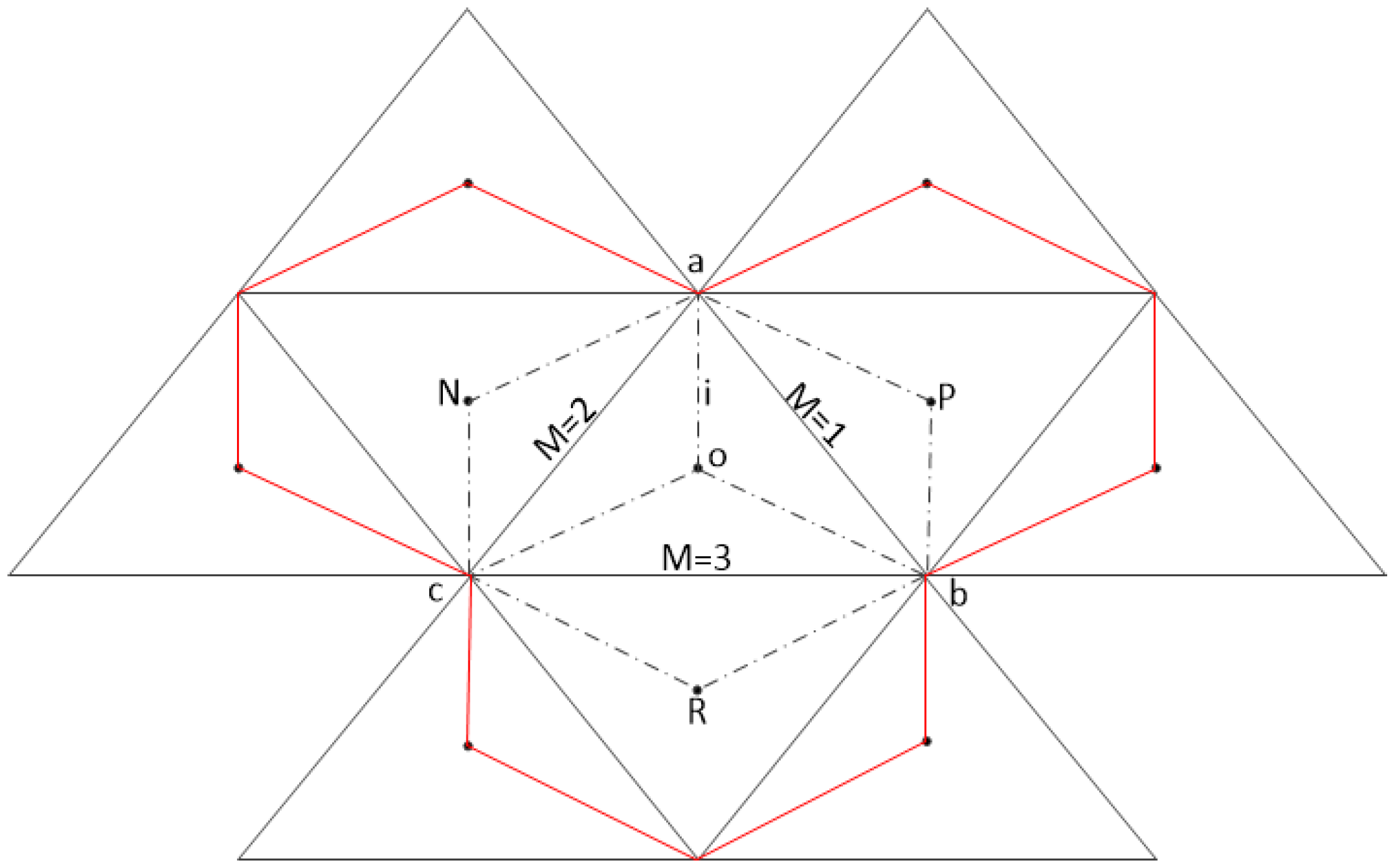
2.2. Slope Term Treatment and Preservation of C-Property

Since the introduction of a well-balanced condition for the shallow-water equations in [17], a number of methods have been proposed with regard to the slope source term treatment. A scheme is regarded to be well-balanced if it satisfies the C-property or maintains quiescent equilibrium over uneven beds. The velocity and water levels for the quiescent state become:

$$u=v\equiv 0\eta =h+z\equiv \mathrm{const}.$$

(21)

Corresponding water levels at the cell center and interface are then given as:

$$h_o+z_o=h_M+z_M$$

(22)

where $h_o,h_M,z_o,z_M$ are respective water depths and bed elevations at cell center and interface. Following [16] we take the slope source term integral over a triangular control volume shown in Figure 1 followed by expressing the integrals in form of fluxes. The slope source flux through the cell can be expressed as a summation of the flux through each interface:

$${\displaystyle \sum _{M=1}^3{\mathit{F}}_{sM}{\mathit{n}}_M{l}_M}={\mathit{F}}_{s1}{\mathit{n}}_1{l}_1+{\mathit{F}}_{s2}{\mathit{n}}_2{l}_2+{\mathit{F}}_{s3}{\mathit{n}}_3{l}_3$$

(23)

where ${\mathit{F}}_{sM}$ denotes the slope source term flux through the interface M and $l_M$ is the length of the interface M. The integral of the slope term over the cell abc can be expressed as:

$${\displaystyle {\int }_{\mathsf{\Omega }abc}\left(-gh\frac{\partial z}{\partial x}\right)}d\mathsf{\Omega }={\displaystyle {\int }_{\mathsf{\Omega }abM}\left(-gh\frac{\partial z}{\partial x}\right)}d\mathsf{\Omega }+{\displaystyle {\int }_{\mathsf{\Omega }bcM}\left(-gh\frac{\partial z}{\partial x}\right)}d\mathsf{\Omega }+{\displaystyle {\int }_{\mathsf{\Omega }acM}\left(-gh\frac{\partial z}{\partial x}\right)}d\mathsf{\Omega }$$

(24)

For demonstration, we estimate the integral over sub-cell abM; the same procedure can be applied to compute flux through other interfaces:

$${\displaystyle {\int }_{\mathsf{\Omega }abM}\left(-gh\frac{\partial z}{\partial x}\right)}d\mathsf{\Omega }=-g\left(\frac{{\tilde{h}}_1+h_o}{2}\right)\left(z_1-z_o\right)$$

(25)

where ${\tilde{h}}_1$ is the average water depth at interface $M=1$,

$${\tilde{h}}_1=\frac{h_{1L}+h_{1R}}{2}$$

(26)

Equation (25) can then be expressed as:

$${\displaystyle {\int }_{\mathsf{\Omega }abM}\left(-gh\frac{\partial z}{\partial x}\right)}d\mathsf{\Omega }=-g\left[\left(\frac{h_{1L}+h_{1R}+2h_o}{4}\right)\left(z_1-z_o\right)\right]$$

(27)

The slope source term flux through all the faces of cell abc can then be given as:

$${\displaystyle {\int }_{\mathsf{\Omega }abc}\left(-gh\frac{\partial z}{\partial x}\right)}d\mathsf{\Omega }=-g\left[\left(\frac{h_{1L}+h_{1R}+2h_o}{4}\right)\left(z_1-z_o\right)+\left(\frac{h_{2L}+h_{2R}+2h_o}{4}\right)\left(z_2-z_o\right)+\left(\frac{h_{3L}+h_{3R}+2h_o}{4}\right)\left(z_3-z_o\right)\right]$$

(28)

For a two-dimensional arbitrary cell, slope source term flux can be expressed as:

$${\mathit{F}}_s\left(\mathit{U}\right).\mathit{n}=\left[\begin{array}{c}0\\ -g\left(\frac{h_{ML}+h_{MR}+2h_o}{4}\right)\left(z_M-z_o\right)n_x\\ -g\left(\frac{h_{ML}+h_{MR}+2h_o}{4}\right)\left(z_M-z_o\right)n_y\end{array}\right]$$

(29)

where $h_{ML},h_{MR}$ are the reconstructed water depths and $z_M$ is the bed elevation at interface M, estimated as:

$$z_M=\max \left(0,{\eta }_L-h_L,{\eta }_R-h_R\right)$$

(30)

The next step is to verify whether the proposed slope source term treatment in Equation (29) balances the convective flux terms represented by E and G in Equation (2). For the motionless steady state given by Equation (21), the convective flux terms become:

$${\mathit{F}}_c\left(\mathit{U}\right).\mathit{n}={\left[0\left(g{h}_M^2/2\right)n_x\left(g{h}_M^2/2\right)n_y\right]}^T$$

(31)

where ${\mathit{F}}_c$ represents the convective fluxes. We use Equation (26) to approximate $h_M$ in Equation (31):

$${\mathit{F}}_c\left(\mathit{U}\right).\mathit{n}=\left[\begin{array}{c}0\\ 1/8g{\left(h_{ML}+h_{MR}\right)}^2{n}_x\\ 1/8g{\left(h_{ML}+h_{MR}\right)}^2{n}_y\end{array}\right]$$

(32)

Making use of the quiescent equilibrium condition expressed in Equation (22), Equation (29) becomes:

$${\mathit{F}}_s\left(\mathit{U}\right).\mathit{n}=\left[\begin{array}{c}0\\ 1/8g\left[{\left(h_{ML}+h_{MR}\right)}^2-{\left(2h_o\right)}^2\right]n_x\\ 1/8g\left[{\left(h_{ML}+h_{MR}\right)}^2-{\left(2h_o\right)}^2\right]n_y\end{array}\right]$$

(33)

Subtracting the convective flux in Equation (32) from the slope source flux in Equation (33) yields:

$${\mathit{F}}_s\left(\mathit{U}\right).\mathit{n}-{\mathit{F}}_c\left(\mathit{U}\right).\mathit{n}=\left[\begin{array}{c}0\\ -1/2g{h}_o^2{n}_x\\ -1/2g{h}_o^2{n}_y\end{array}\right]$$

(34)

Since we have converted the slope source terms into flux through the interface, Equation (8) can also be written as

$${\mathit{U}}_{ij}^{n+1}={\mathit{U}}_{ij}^n-\frac{△t}{A}\left[{\displaystyle \sum _{M=1}^3{\mathit{F}}_c{({\mathit{U}}_M^L,{\mathit{U}}_M^R)}^{n+1/2}.{\mathit{n}}_M{L}_M}-{\displaystyle \sum _{M=1}^3{\mathit{F}}_s{(\mathit{U})}^{n+1/2}.{\mathit{n}}_M{L}_M}\right]$$

(35)

Friction source terms are discretized separately using an explicit scheme; therefore, they are disregarded in Equation (35). Differences in the slope source and convective flux given by Equation (34) are introduced in Equation (35):

$$\begin{array}{cc}\hfill {\mathit{U}}_{ij}^{n+1}& ={\mathit{U}}_{ij}^n-\frac{△t}{A}{\displaystyle \sum _{M=1}^3\left[\begin{array}{c}0\\ 1/2g{h}_o^2{n}_{xM}{l}_M\\ 1/2g{h}_o^2{n}_{yM}{l}_M\end{array}\right]}\hfill \\ & ={\mathrm{U}}_{ij}^n-\frac{1}{2}g{h}_o^2\frac{△t}{A}{\displaystyle \sum _{M=1}^3\left[\begin{array}{c}0\\ n_{xM}{l}_M\\ n_{yM}{l}_M\end{array}\right]}\hfill \end{array}$$

(36)

Since ${\displaystyle \sum _{M=1}^3{n}_{xM}{l}_M}={\displaystyle \sum _{M=1}^3{n}_{yM}{l}_M}=0$, Equation (36) becomes:

$${\mathit{U}}_{ij}^{n+1}={\mathit{U}}_{ij}^n$$

(37)

which is the primary requirement of a motionless steady flow. Equation (37) shows that the proposed source term treatment preserves the quiescent equilibrium perfectly. Equation (36) may seem similar to Equation (30) in [26], but is based on a different mathematical formulation and slope source flux computation through the interface. The proposed method of considering the reconstructed water depth at both sides of the interface in averaging water depths for source terms and convective flux serves to eliminate any chance for instabilities to arise due to a discontinuity of conserved variables at an interface caused by abrupt change in bed elevation. Our method is also able to obtain appropriate water depth averages at interfaces for both structured and unstructured meshes, which is verified through test case simulations. We demonstrated through several theoretical cases that the well-balanced conditions were perfectly preserved by the proposed slope source treatment.

2.3. Wet–Dry Front Treatment

To prevent unphysical high velocity and negative water depth at the wet–dry interface, we adopt a hydrostatic reconstruction procedure proposed in [22]. The bed elevation at the interface between two cells is chosen as:

$$z_M=\max (z_L,z_R)$$

(38)

where $z_L,z_R$ are the bed elevations at left and right of the interface, respectively. After selecting the higher bed elevation at the interface, the bed elevation is modified by the following step:

$$z_M=\min (z_M,h_L+z_M)$$

(39)

Water depths and velocities at left and right side of the interface are then evaluated as:

$$\begin{array}{c}{h}_{MR}=\max (0,{\eta }_{MR})-\max (0,z_M-z_{MR})\\ h_{ML}={\eta }_L-z_M\\ u_{ML}=\frac{q_{ML}}{h_{ML}};u_{MR}=\frac{q_{MR}}{h_{MR}}\end{array}$$

(40)

2.4. Boundary Conditions

Boundary conditions are implemented in the ghost cells outside the computational domain at inlet and outlet for all test cases. Following the theory of characteristics, two boundary conditions among the three flow variables ($\eta ,q_x,q_y$) are specified for subcritical flows, and in case of supercritical flows all three flow quantities are specified in ghost cells. Depending upon the outflow conditions, transmissive and solid reflective boundary conditions are considered at the outlet.

3. Model Applications

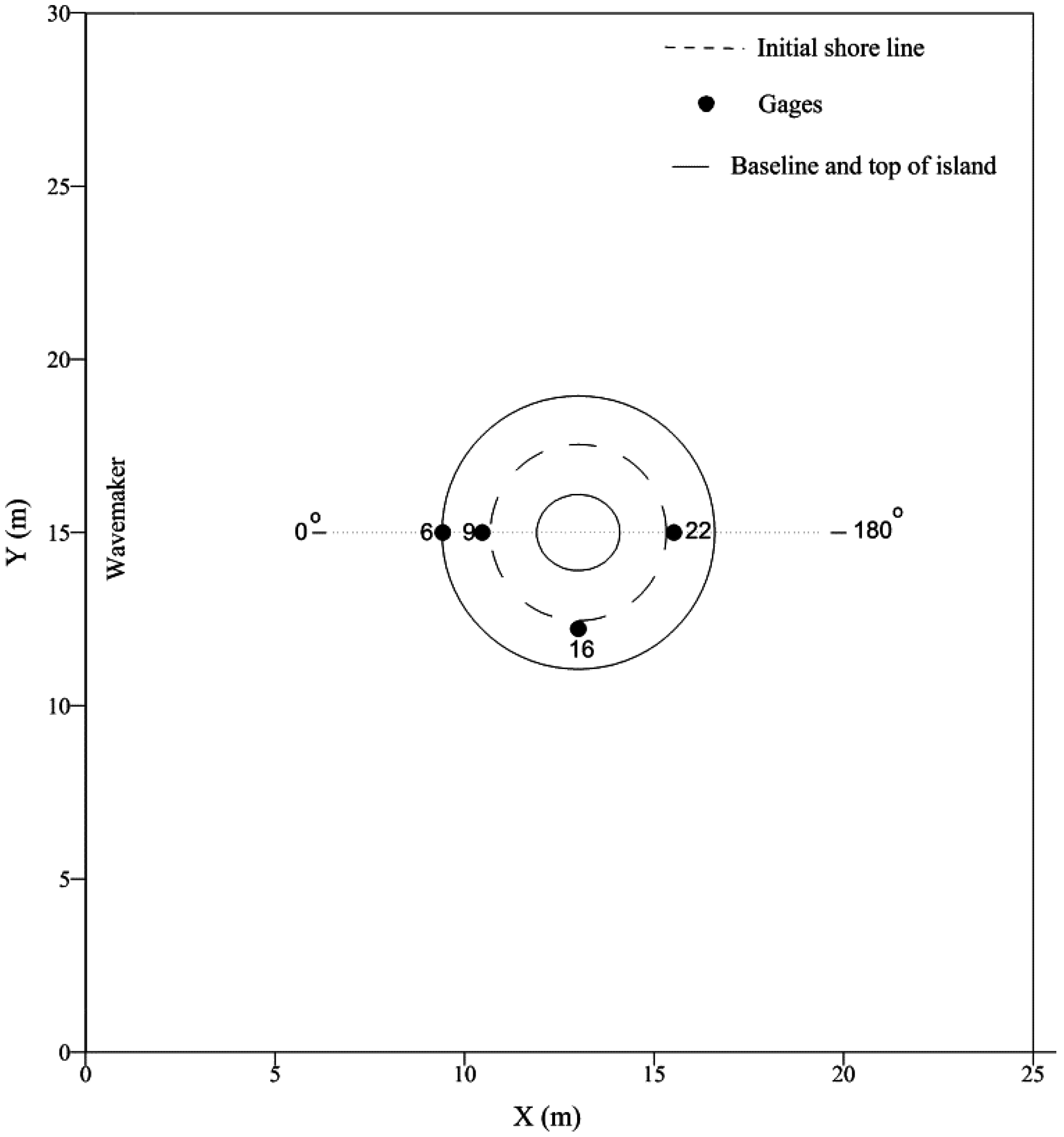
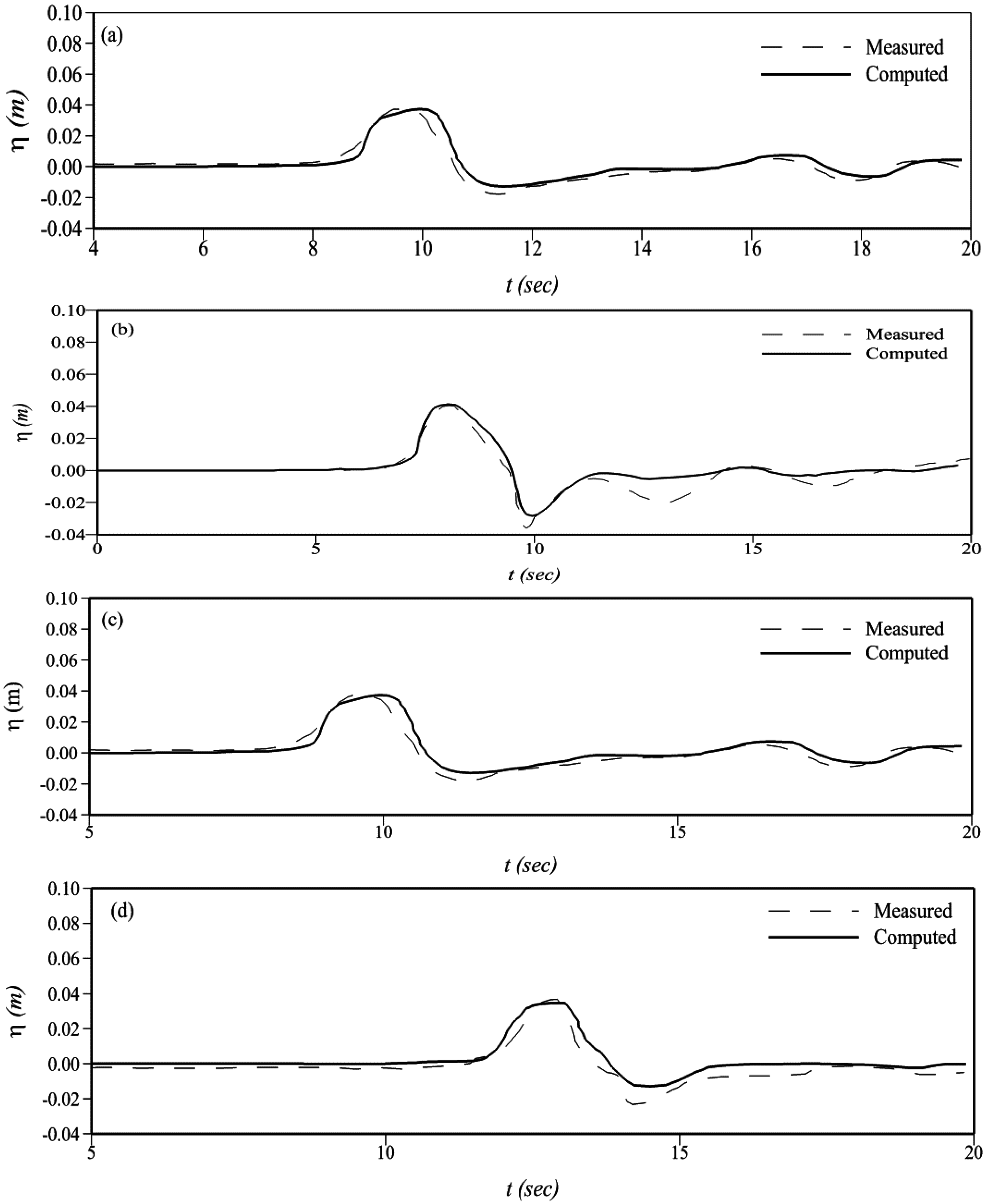
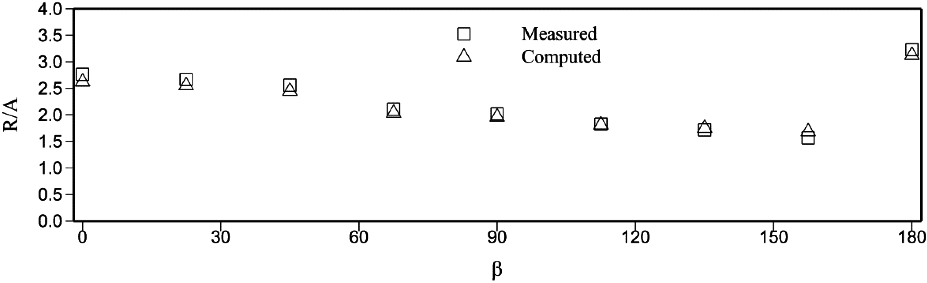
3.1. Solitary Wave Interaction with Conical Island

Non-linear SWEs have been validated by several researchers in the coastal engineering community [4,31,32] for nearshore tsunami propagation, including the benchmark case of a solitary wave run-up over a conical island proposed by Briggs et al. [33]. The unexpectedly large tsunami heights observed at circular-shaped Babi Island and pear-shaped Okushiri Island (1993) motivated researchers to explore the interactions of solitary waves with conical islands.

Experiments were carried out at the US Army Corp of Engineers, Coastal and Hydraulics Laboratory. A 30 m-wide and 25 m-long basin was used with a truncated circular cone as an island in the center. The conical island had base and top diameters of 7.2 m and 2.2 m, respectively, and a height of 0.625 m. Solitary waves were generated by a directional spectral wave generator (DSWG) installed along the long axis of the basin. A schematic of the experimental set up can be seen in Figure 2. The experiment was performed for water depths of 0.32 m and 0.42 m, and solitary wave heights varied between 0.05 m and 0.1 m.

In this study, we modeled a solitary wave height of $\zeta$ = 0.032 m propagating over an initial water depth of h = 0.32 m ($\zeta$/h = 0.1 m). The discretized domain consisted of 2577 elements; the CFL number was set to 0.6, and the Manning’s roughness coefficient was taken as 0.016 for the concrete surface of the basin and island. To emulate the experimental conditions, radiation boundary conditions were applied at lateral boundaries to reduce wave reflection that could interact with the propagating wave. At x = 0, the solitary wave was generated by specifying the free surface elevation and velocity [4,34]:

$$\eta (x,t)=A\sec {\mathrm{h}}^2\sqrt{\frac{3A}{4h^3}}\left(x-ct\right)$$

(41)

$$u(t)=\eta (x,t)\sqrt{\frac{g}{h}}$$

(42)

where c is the wave celerity equal to $\sqrt{g(h+A)}$. There were 27 gauges in the experimental set up to record wave positions with time. We compared the computed results with the measured results at four gauge locations in Figure 3. The model was run for 20 s because afterwards the wave motion becomes dispersive [4,33].

A time series of water surface elevations obtained from our proposed model was compared with the measured values at four gauges; the comparisons can be seen in Figure 3. The wave arrival time was well predicted at all gauges. The predicted overall wave shape is in general agreement with the experimental observations; however, due to the non-dispersive nature of the non-linear SWEs a steeper wave is observed at gauges 6, 9 and 16. This wave front shape was also observed in prior studies that modeled tsunami propagation by SWEs [4,31]. The depression that followed the lead wave and the secondary depressions are underestimated at gauges 6, 9, and 22; this is consistent with results reported by [35]. Observations at gauges 9 and 22 show that the measured free surface elevation remains below the still water depth for a considerably longer time than the model simulation, predicting that the free surface elevation approaches the still water depth faster and maintains that profile. The leading wave at gauge 16 has a slightly wider crest that causes a delayed depression, but the overall waveform and amplitude values are in good agreement.

A comparison of the maximum predicted and measured run-ups around the island is shown in Figure 4. β is the angle measured counter-clockwise to the island, and R is the maximum run-up. We observe a trend with regard to the run-up being over-predicted for β between 0° and 65° (the front of the island); however, from 90° to 120°, the predicted results are in good agreement with the experiment until the wave reaches the back of the island where we observe a gradual increase in the under-estimation of run-up heights. The overall agreement between the computed and measured values shows that our proposed scheme could adequately model tsunami propagation and the various processes associated with it, including: wave breaking, shoaling, reflection, run-ups and run-downs.

3.2. Dam-Break Flow in an L-Shaped Channel

We considered the flow behavior in an L-shaped channel with a 90° bend. Flow within the bend shows strong two-dimensional features, making it suitable for assessing the two-dimensional modeling capabilities of our numerical scheme. The channel was discretized into 3948 unstructured elements and 2132 nodes, shown in Figure 5. The reservoir bed was 0.33 m below the channel bed and a friction coefficient of 0.019 was assumed over the entire domain. Based on the experimental studies of [36], an initial water depth of 0.58 m was contained in the reservoir while the channel bed is dry. A dam at x = 2.39 m separated the reservoir from the channel.

At t = 0.0 s, the dam was suddenly removed and supercritical flow was induced; the simulations were run for 15 s. Propagation of the wave front within the channel, its reflection from the bend, and resulting bore propagation can be seen in Figure 6 at t = 6 and 15 s.

The wave reached the bend approximately 6 s after the dam-break, as shown in Figure 6a, followed by an upstream travelling reflection and a depression in the water surface elevation immediately downstream from the bend. The reflected bore smoothly propagated upstream without exhibiting any oscillatory behavior at t = 15 s after the dam-break, as shown in Figure 6b. Model prediction for the water depth in the channel was further compared with the experimental observations in [36] and the published numerical results of [37] in Figure 7, at t = 3, 5, 7, and 14 s. It is evident that our scheme achieves a very satisfactory agreement with the experimental observations, demonstrating that it could satisfactorily model two-dimensional supercritical flows involving bends and sudden directional changes.

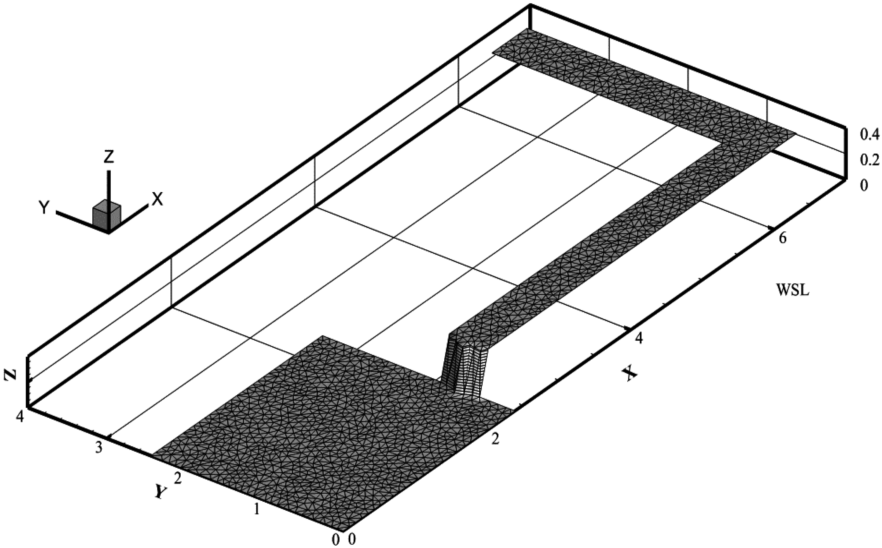
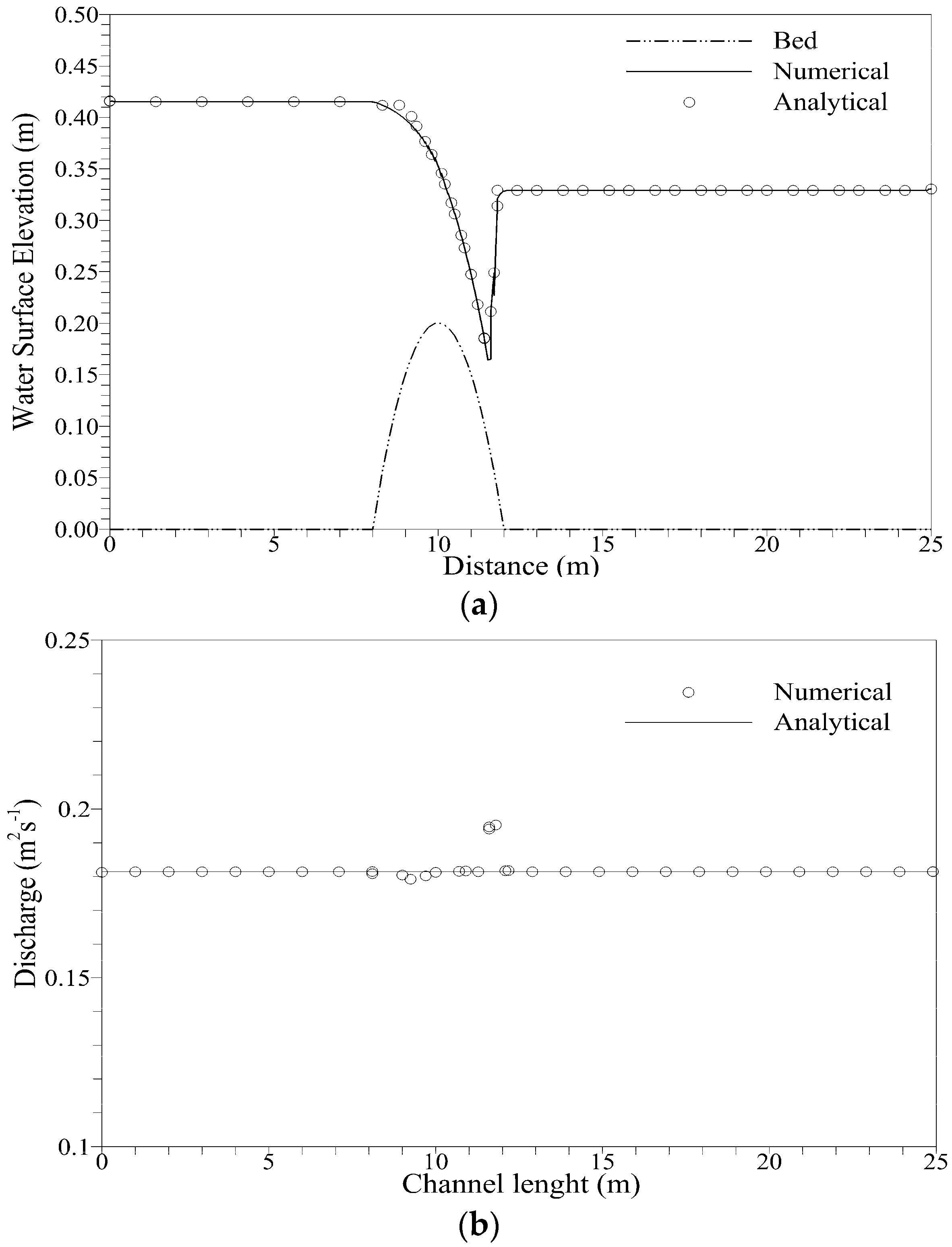
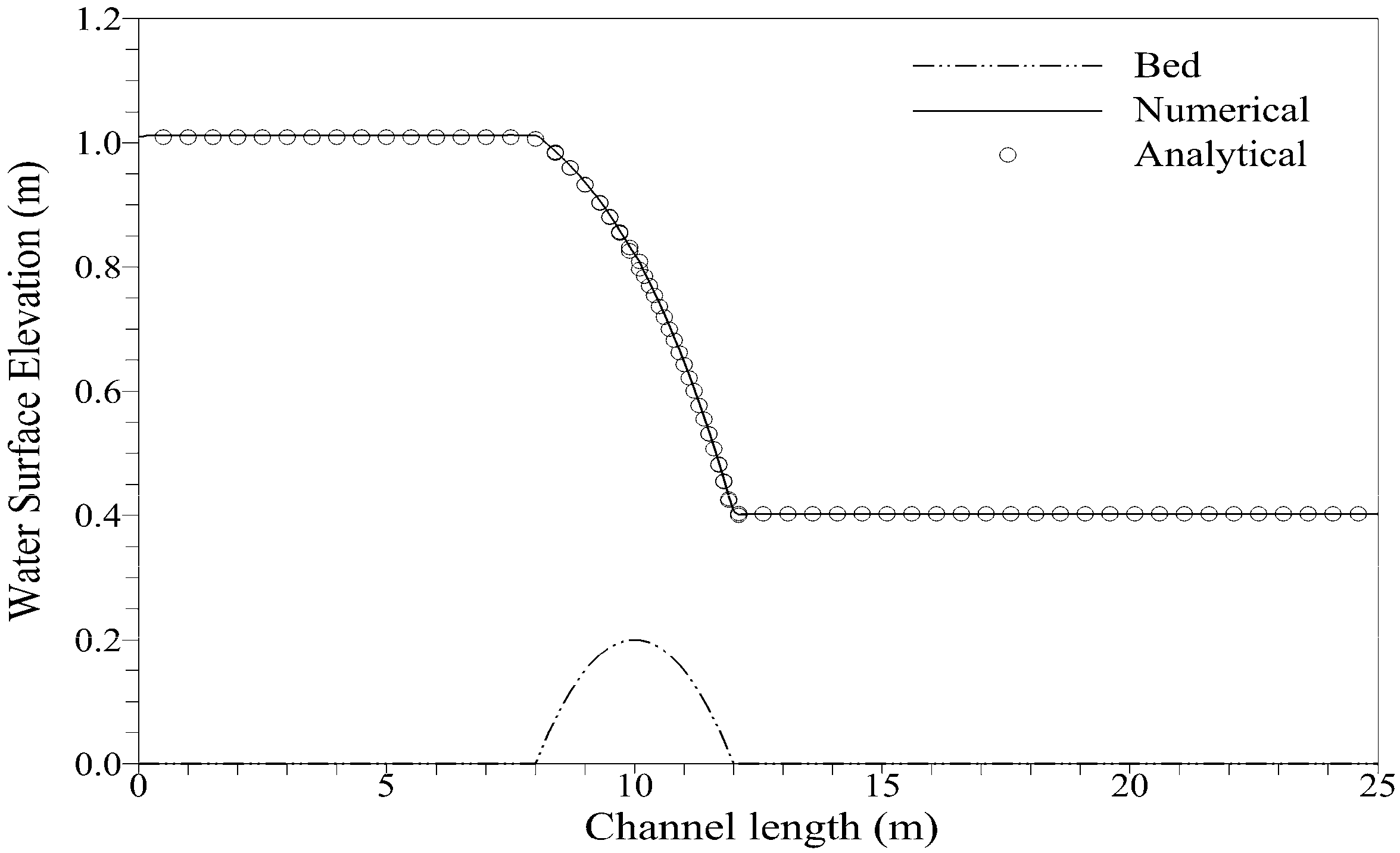
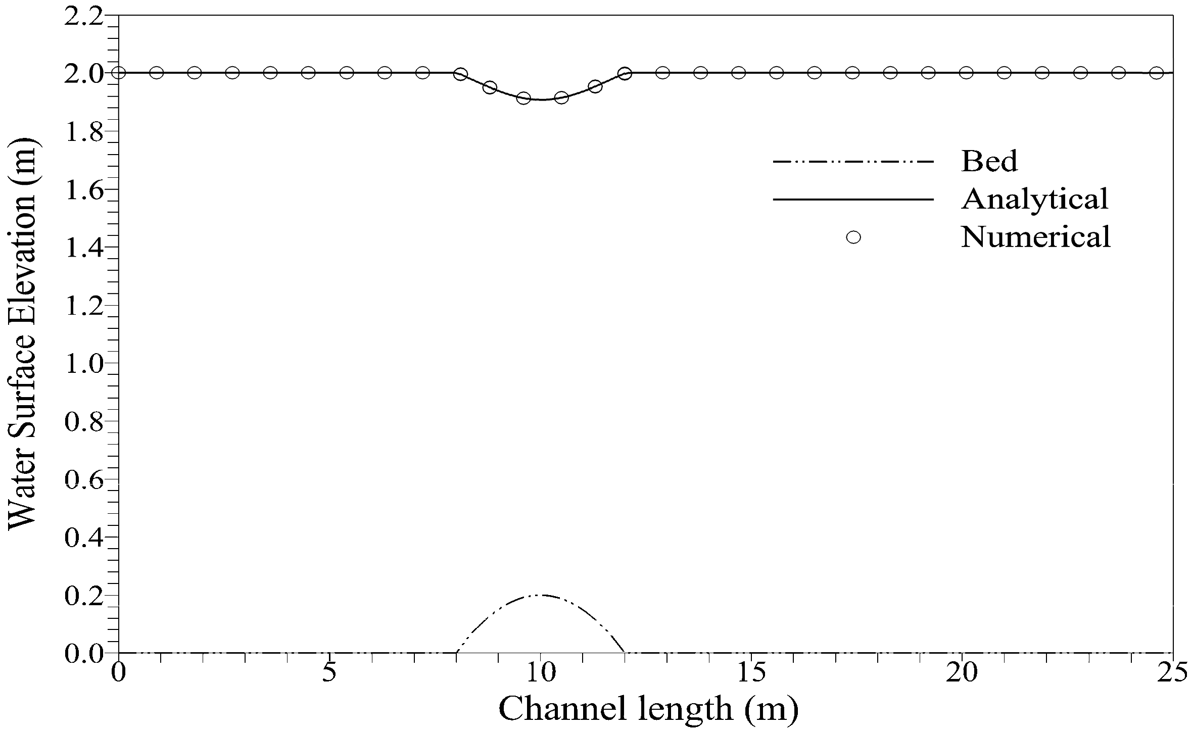
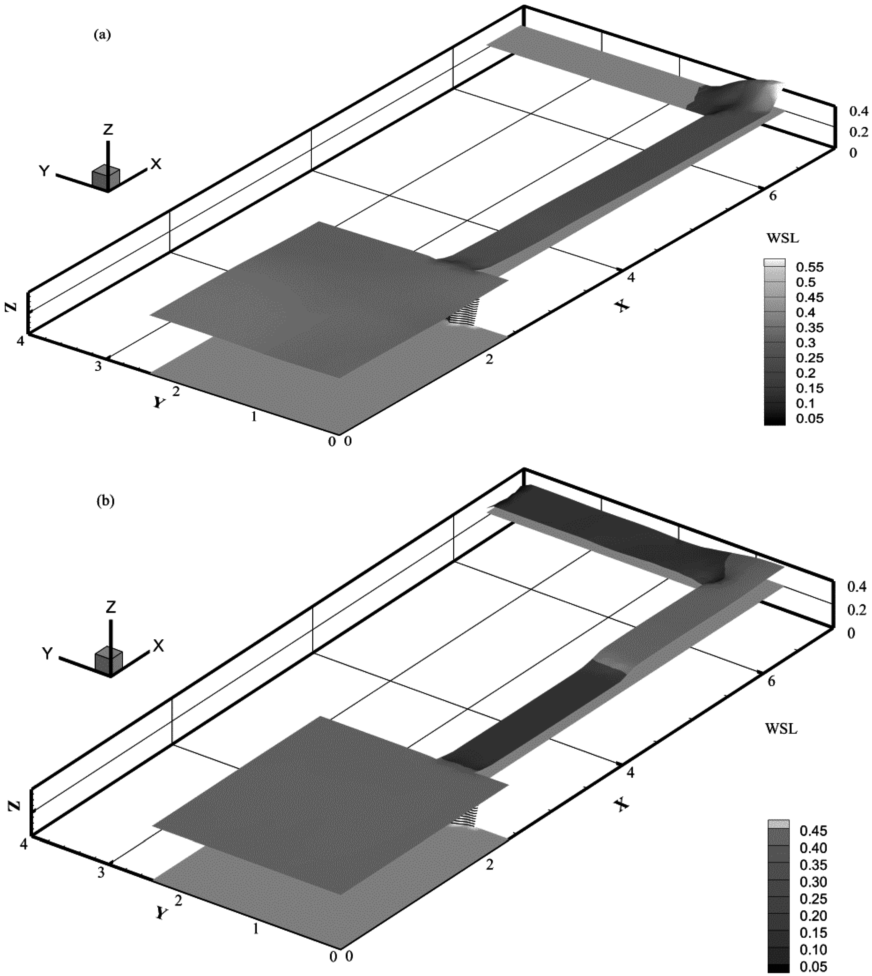
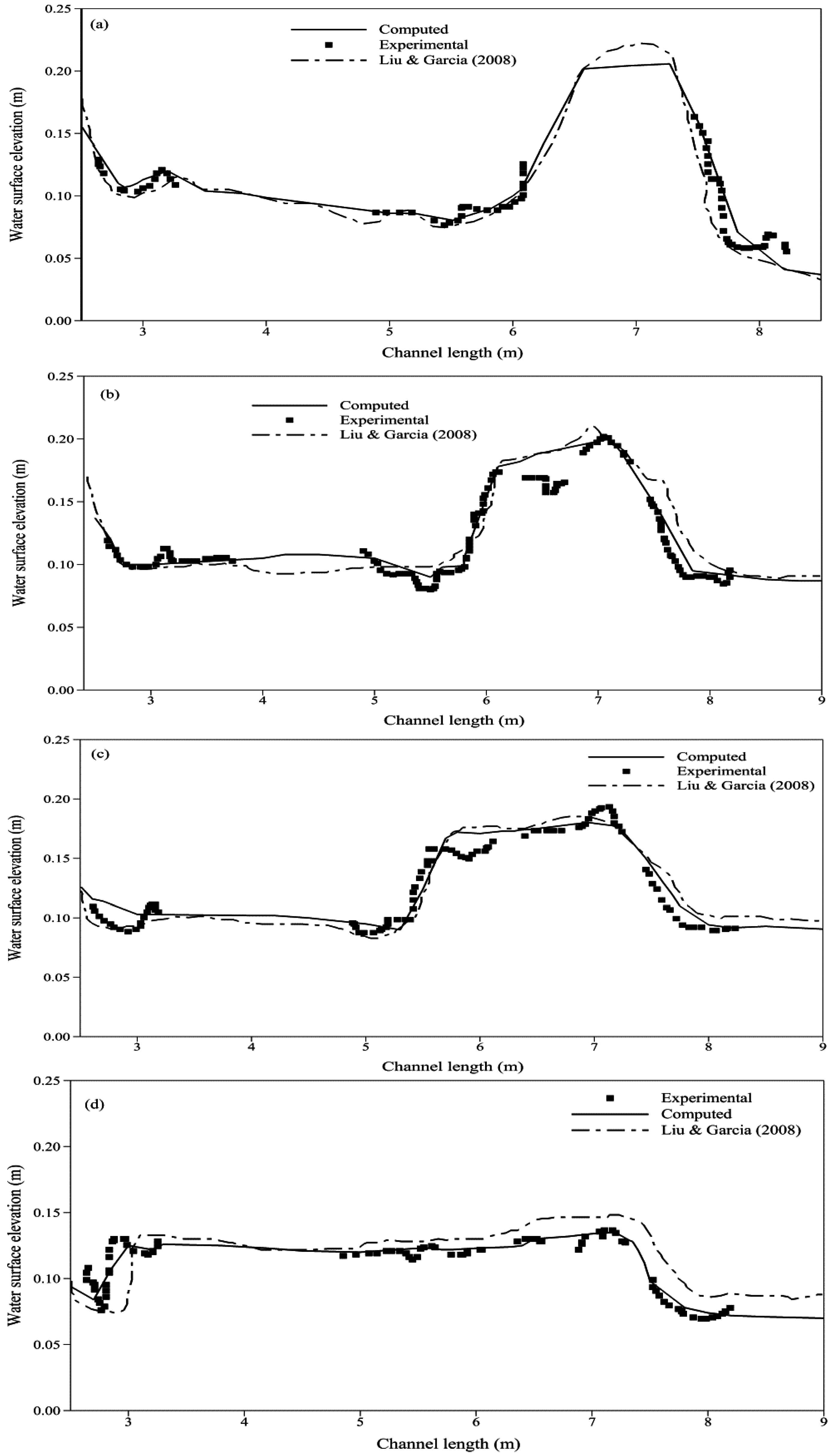
3.3. Flow over a Hump

This test problem is widely used to verify well-balanced property of a numerical scheme towards moving steady state solution [7,8,25]. The moving steady-state water equilibrium is given by:

$$m:=hu=\mathrm{const}.;E:=\frac{1}{2}{u}^2+g\left(h+z\right)=\mathrm{const}.$$

(43)

where m and E are equilibrium variables. The bed profile of a 25 m-long and 0.1-m wide channel with a bump is defined as

$$z_b(x)=\{\begin{array}{ll}0.2-0.05{(x-10)}^2& \mathrm{if}8<x<12\\ 0& \mathrm{otherwise}\end{array}$$

(44)

Boundary conditions are adjusted to generate subcritical flow with a shock, or a transcritical flow with or without a shock. The domain is treated as two-dimensional by discretizing with unstructured triangular cells and the CFL number of 0.6 was maintained for all cases.

3.3.1. Transcritical Flow with a Shock

We simulate a transcritical flow with a shock by setting a water depth (0.33 m) and discharge (q_x = 0.18 ms⁻²) at the left and right boundaries, respectively. The initial conditions are fixed as:

$$\begin{array}{l}E=\{\begin{array}{ll}\frac{3}{2}{\left(9.812\times 0.18\right)}^{\frac{2}{3}}+9.812\times 0.2& \mathrm{if}x\le 11.67\\ \frac{{0.18}^2}{2\times {0.33}^2}+9.812\times 0.33& \mathrm{otherwise}\end{array}\\ m=0.18\end{array}$$

(45)

3.3.2. Transcritical Flow without a Shock

The initial conditions are fixed as:

$$\begin{array}{l}E=\{\frac{{1.53}^2}{2\times {0.66}^2}+9.812\times 0.66\\ m=1.53\end{array}$$

(46)

At upstream boundary a discharge of 1.534 ms⁻² is imposed and a water depth of 0.66 m is imposed at downstream boundary.

3.3.3. Subcritical Flow

The initial conditions are fixed as:

$$E=22.067,m=4.42$$

(47)

At upstream boundary a discharge of 4.42 ms⁻² is imposed and a water depth of 2 m is imposed at the downstream boundary.

For steady states, the initial condition given in Equations (43), (45) and (46) should be exactly preserved. We run the simulations for 20.0 s; comparisons of the numerical results for the water surface elevation and discharge with the analytical solution were in excellent agreement, as shown in Figure 8, Figure 9 and Figure 10. The comparison of numerical and analytical solutions shows excellent agreement; however, discharge for flow with shock in Figure 8 shows discrepancy with the analytical solution at x = 12 m, which is where shock is generated. This disagreement was also observed previously in [20,28,38]. We measured convergence of solution for transcritical flow with a shock by using global relative error:

$$R\left(h\right)=\sqrt{\frac{{\displaystyle \sum _i^N\left[A_i{\left(\frac{h_i^n-h_i^{n-1}}{h_i^n}\right)}^2\right]}}{{\displaystyle \sum _i^N{A}_i}}}$$

(48)

where $h$ is water depth; i is cell number, N is the total number of cells; n is time level; and A is the area of cell i. To demonstrate that the steady state is exactly preserved we measure $L^1$ error for water height and discharge for all three cases at t = 20 s. The values in

Table 1. $L^1$ error-norm for flow variables over a hump.

Flow Type	h	${\mathit{q}}_{\mathit{x}}$
Transcritical flow with a shock	$5.02\times {10}^{-4}$	$7.83\times {10}^{-4}$
Transcritical flow without a shock	$2.83\times {10}^{-4}$	$7.23\times {10}^{-4}$
Subcritical flow	$1.81\times {10}^{-4}$	$5.02\times {10}^{-4}$

show smaller deviation between numerical and exact solutions of water depth than for discharge which is due to discrepancy between exact and numerical discharge immediately downstream of the hump, however, the overall agreement between computed and exact solution is satisfactory.

Comparison of convergence rates for transcritical flow with a shock in Figure 11 shows improvement by the proposed method where convergence is reached after 15,000 iterations. For SGM [20] and RSGM [7] methods, convergence is achieved after 16,000 and 15,600 iterations, respectively.

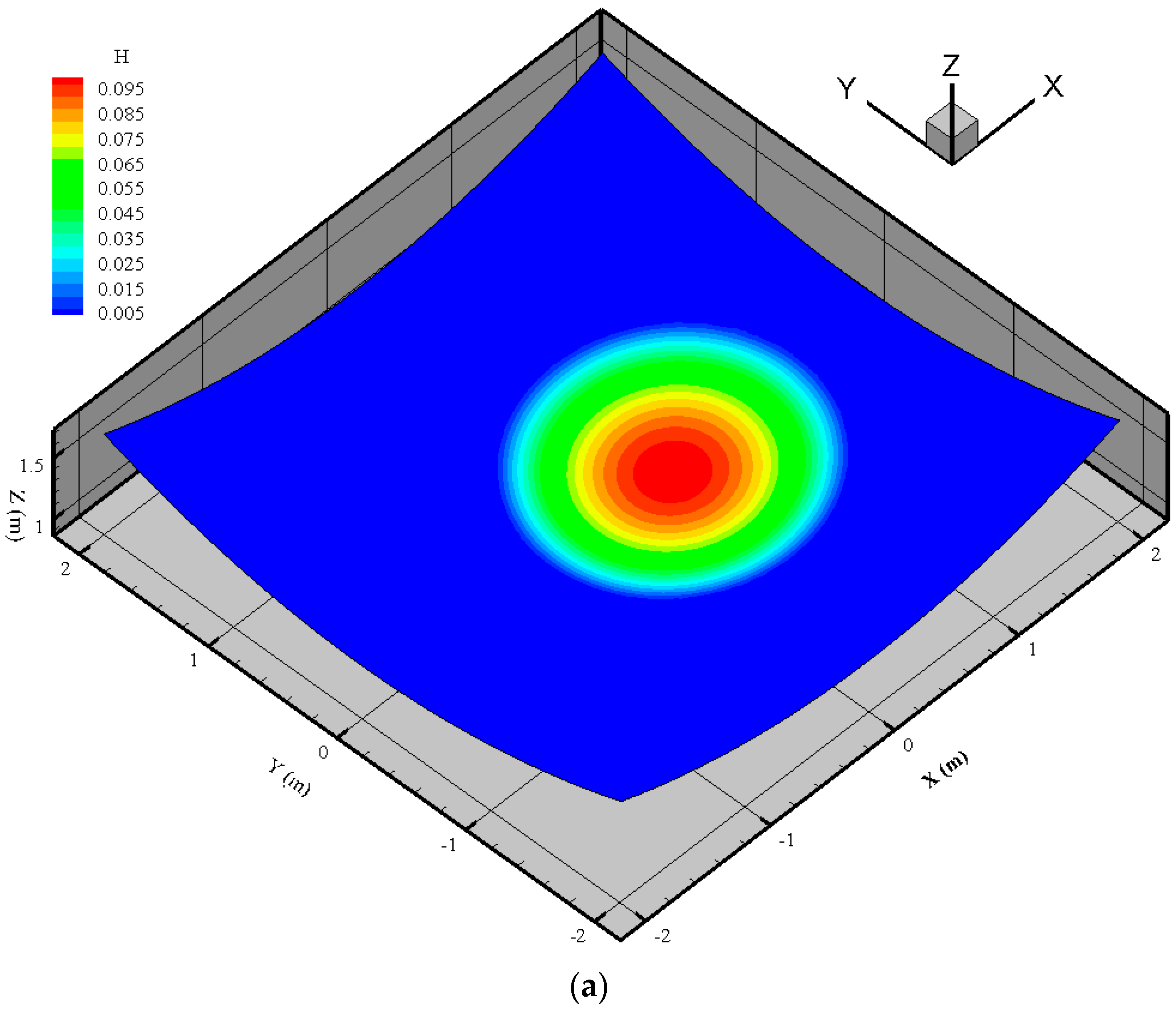
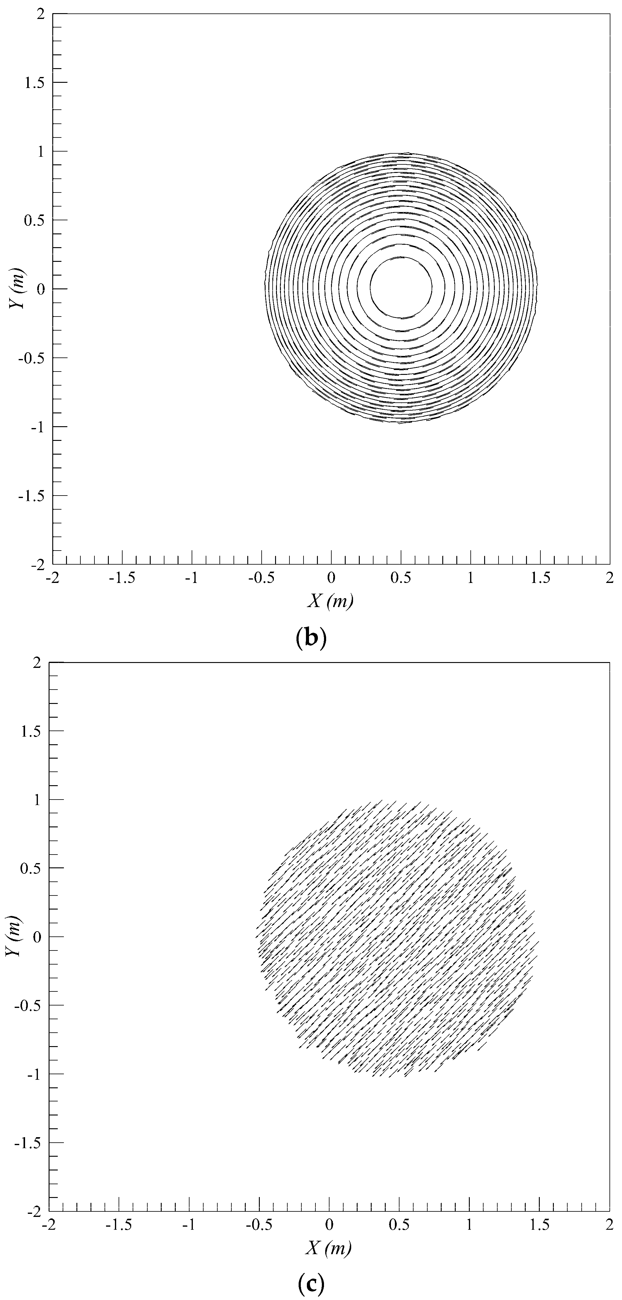
3.4. Thacker’s Planar Solution

Flow inside a parabolic basin is an important test case in hydraulics and coastal engineering, modelled by a number of researchers [4,24,26] for testing the ability of the model to handle wet–dry fronts over uneven beds. Simulating flow inside a parabola is challenging because of periodic wetting and drying involving run-up and run-down. We verify the wet–dry front handling ability of our model by considering a parabolic computational domain of 4 m × 4 m with a frictionless bottom. Geometry of the domain is given by the equation:

$$z(x,y)=1-h_o\left[1-\frac{x^2+y^2}{a^2}\right]$$

(49)

where $h_o$ is the water depth at center of domain and a is the distance from center to zero elevation of shore. The analytical solution to the problem is given as [39]:

$$\begin{array}{l}h(x,y,t)=1+\frac{\sigma h_o}{a^2}\left[2x\cos (\omega t)+2y\sin (\omega t)-\sigma \right]\\ u(t)=-\omega \sigma \sin (\omega t),v(t)=\omega \sigma \cos (\omega t)\end{array}$$

(50)

where $\sigma$ is the amplitude parameter fixed equal to 0.5; $\omega$ represents rotational frequency given by $\sqrt{2g{h}_o/a^2}$; other parameters are set as $h_o$ = 0.1 m, a = 1.0 m. Initial conditions are set by evaluating Equation (50) at t = 0. Time period of water sloshing in the basin is given by the equation:

$$T=\frac{2\pi }{\omega }$$

(51)

Water surface elevations and velocity results obtained from numerical scheme are compared with the analytical solution at time 4T, shown in Figure 12. The comparisons show very good agreement between numerical results and analytical solution for water levels at y = 2 m. The comparison of vector field provided for velocity show that very small perturbations exist near the wet–dry front, but importantly we observed that those perturbations do not affect the accuracy of the solution by growing in time; moreover, it has been observed in previous studies too, that small perturbations near the wet–dry front are very difficult to remove. The shoreline propagates smoothly between wet–dry surfaces with no spurious oscillations which indicate that water depth and velocity at wet–dry interfaces are estimated accurately with a hydrostatic reconstruction method and proposed treatment of slope source terms.

To assess the asymptotic order convergence for water depth h and velocity u, we measure the errors in terms of $L_1$ and $L_2$ norms for successively refined unstructured grids. The error norms are computed by the following equation:

$$L_p={\left(\frac{{\displaystyle \sum _{k=1}^N\left|A_k\right|{\left(T_k^{numerical}-T_k^{analytical}\right)}^p}}{{\displaystyle \sum _{k=1}^N\left|A_k\right|}}\right)}^{\frac{1}{p}};p=1,2$$

(52)

where p is the error norm being measured; T is the flow variable, in this case water depth h and velocity u; A is the area of the cell, and N is the total number of elements in the mesh.

Table 2. Grid properties and error-norm for Thacker’s planar solution.

Line Segments in x- and y-Directions ${\mathit{N}}_{\mathit{x}}={\mathit{N}}_{\mathit{y}}$	Total Number Grid Points ${\mathit{N}}_{\mathit{g}}$	Characteristic Length for Each Grid ${\mathit{L}}_{\mathit{N}}=\sqrt{\frac{4\times 4}{{\mathit{N}}_{\mathit{g}}}}(\mathbf{m})$	${\mathit{L}}_1$ Norm		${\mathit{L}}_2$ Norm
			$\mathit{h}(\mathbf{m})$	$\mathit{u}(\mathbf{m}{\mathbf{s}}^{-1})$	$\mathit{h}(\mathbf{m})$	$\mathit{u}(\mathbf{m}{\mathbf{s}}^{-1})$
$16$	$372$	$0.21$	$-2.48\times {10}^{-7}$	$-1.86\times {10}^{-3}$	$2.98\times {10}^{-4}$	$4.27\times {10}^{-3}$
$32$	$1511$	$0.1$	$-2.33\times {10}^{-7}$	$-1.88\times {10}^{-3}$	$3.07\times {10}^{-4}$	$4.32\times {10}^{-3}$
$64$	$6072$	$0.051$	$-2.02\times {10}^{-8}$	$-1.93\times {10}^{-3}$	$3.09\times {10}^{-4}$	$4.36\times {10}^{-3}$

shows the properties of successively refined grids and values of error norms for water depth and velocity. We observe behavior in values of error norms for both flow variables since only distorted unstructured grids are used to check the convergence.

Mass conservation of the solution is verified by the following equation:

$${\epsilon }_m={\max }_t\left(\frac{\left|V_t-V_o+\delta V_t\right|}{V_o}\right)$$

(53)

where $V_o$ and $V_t$ are the volume of water initially and after time t, respectively, and $\delta V_t$ is the difference between initial and final volume of water. For flow inside the parabola $\delta V_t=0$, because there is no flow through the boundaries. If the water depth in cells, classified as dry by the threshold limit, is set to zero it will lead to subtraction of water volume from the total system which results in non-conservation of mass. Therefore, to preserve mass exactly, after identifying the cells with water depth $0\le h\le {10}^{-5}$ m, we find the volume of water in those cells before setting the water depth to zero. This volume of water is then added to the volume in the neighboring wet cells at every time step. This step preserves the mass conservation exactly. The maximum relative mass error computed with Equation (53) is $4.9\times {10}^{-14}$, which is accurate up to round-off error and confirms the mass conservation.

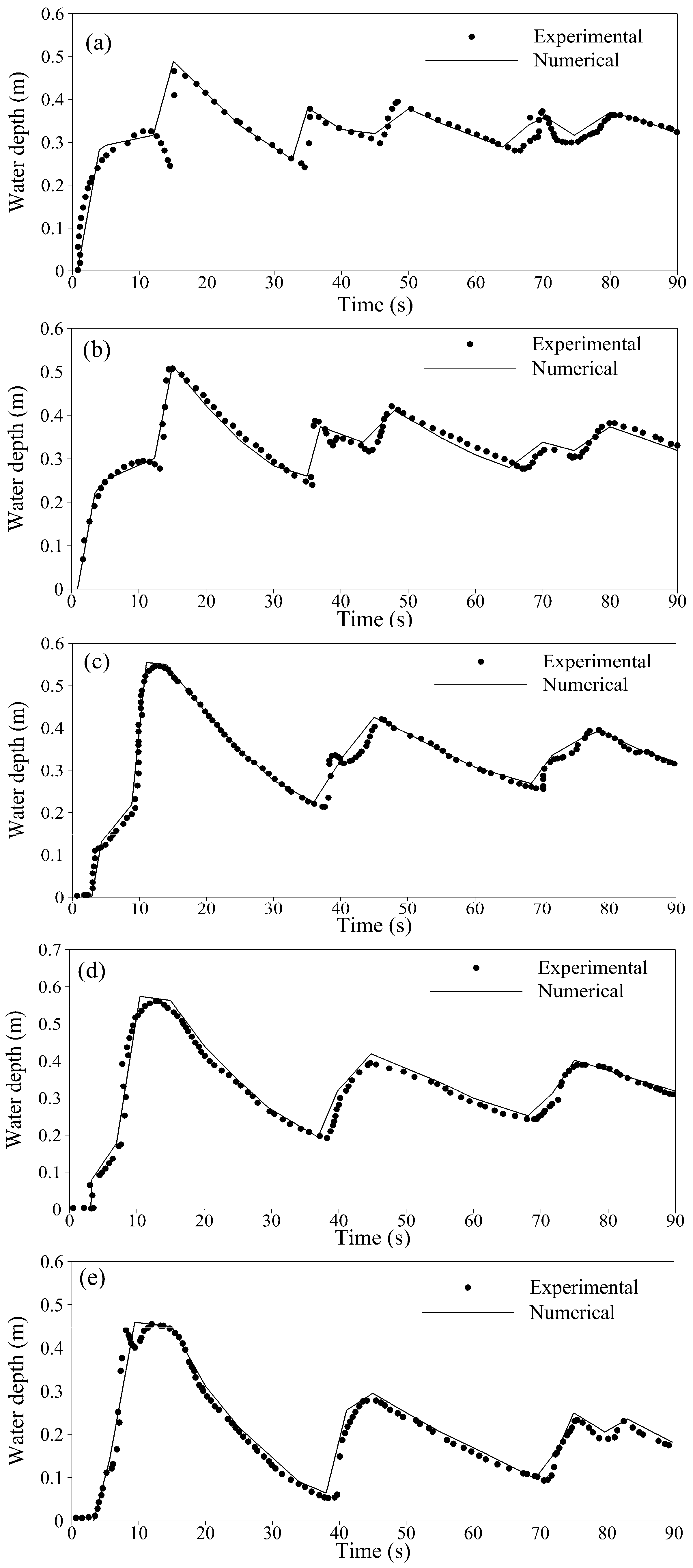
3.5. Dam-Break over a Triangular Obstacle

This test case models the complicated interactions of shock and rarefaction waves, to test the shock handling and propagation of the proposed scheme. This case was previously modeled in [1,7,24] to validate their numerical schemes. A thin wall acting as a hypothetical dam was positioned 15.5 m from the left boundary. To generate a shock wave, a triangular obstacle 0.4 m high and 6 m wide was installed 10 m downstream from the dam.

The computational domain discretized into 2590 elements is shown in Figure 13. The water depth was set to 0.75 m upstream, and 0 m downstream from the dam. Free outfall and solid boundary conditions were imposed on the left and right boundaries, respectively. The laboratory experiment was performed by EU CADAM in a 38 m-long channel with a Manning’s roughness coefficient equal to 0.0125. The simulation results after 90 s were compared with the experimental observations in Figure 14 at seven gauges, located at 2 m, 4 m, 8 m, 10 m, 11 m, 13 m, and 20 m downstream from the dam.

Due to the relative closeness of gauges 1 and 2, almost similar water depth profiles were observed. We observed a gradual increase in water depth on an initially dry bed until approximately 12 s, after which there was an abrupt increase in depth caused by a propagating shock wave reflected from the triangular obstacle. However, the right moving rarefaction wave caused an almost linear draw down in water depth for up to 32 s for gauge 1 and 35 seconds for gauge 2. At that instant, the second shock wave (reflected from the triangular obstacle) again generated an increase in water depth at gauges 1 and 2. However, this time the maximum water depth was lower than before due to the dissipation of energy by friction. The interaction of a rarefaction wave again caused a drop in water level, until the third shock wave reached gauges 1 and 2 at around 45 s.

This wave interaction process continued until all the energy was dissipated and the mass losses due to transmissive flow at the downstream boundary made the flow steady. The same wave propagation processes and interactions were also observed at gauges 3–7. An observed trend in the numerical computations was the early arrival of the second-to-last shock for gauges 1 and 2, and the last shock for the other gauges. This could be due to inaccurate estimation of wave speeds in the HLLC flux computation, causing the waves to travel too fast. However, this was not certain, since the arrival times of the other shocks and rarefaction waves were accurately predicted. Another source for the discrepancy could be error in the experimental observations; there was no consistency in the observations plotted between 65 and 90 s by Liang and Marche [1], observations were both on the higher and lower side. In such a case, the choice of plotting higher or lower observations may affect the resultant comparisons.

Regardless of this small discrepancy, the overall agreement between the numerical results and experimental observations was satisfactory, showing that our scheme is capable of modeling complex wave interactions and wetting/drying.

4. Conclusions

In this paper, we introduced a new, accurate, well-balanced numerical scheme for shallow-water flows using a high-resolution Godunov-type finite volume method. The proposed slope source term discretization is based on averaging water depths at the cell center and reconstructed water depths at both sides of the interface and multiplying this with the difference in bed elevation between the cell center and interface. Applying the model to numerical examples shows that the proposed interpretation of slope source terms can accurately maintain well-balanced conditions for still water. Results from wave run-up/run-down on the conical island and dam-break over triangular obstacle indicate that the proposed scheme can accurately handle wet–dry fronts. Flow over the hump demonstrates that the slope source term exactly balances convective fluxes maintaining a well-balanced condition. The proposed model is tested for various benchmark coastal and hydraulic engineering cases; comparisons between the experimental, analytical, and published numerical results show that the scheme is robust and has a wide range of applications with very satisfactory modeling capabilities for a wide variety of mesh types. Based on the results of several test cases, we can confidently predict that application of the proposed method with regard to slope source term discretization for complicated flow problems (real life and laboratory) will result in well-balanced and accurate solutions.

References

1. Liang, Q.; Marche, F. Numerical resolution of well-balanced shallow water equations with complex source terms. Adv. Water Resour. 2009, 32, 873–884. [Google Scholar] [CrossRef]
2. Audusse, E.; Bristeau, M.-O. A well-balanced positivity preserving “second-order” scheme for shallow water flows on unstructured meshes. J. Comput. Phys. 2005, 206, 311–333. [Google Scholar] [CrossRef]
3. Mohammadian, A.; Le Roux, D.Y. Simulation of shallow flows over variable topographies using unstructured grids. Int. J. Numer. Methods Fluids 2006, 52, 473–498. [Google Scholar] [CrossRef]
4. Hubbard, M.E.; Dodd, N. A 2D numerical model of wave run-up and overtopping. Coast. Eng. 2002, 47, 1–26. [Google Scholar] [CrossRef]
5. Rehman, K.; Cho, Y.-S. Bed evolution under rapidly varying flows by a new method for wave speed estimation. Water 2016, 8, 212. [Google Scholar] [CrossRef]
6. Hou, J.; Simons, F.; Liang, Q.; Hinkelmann, R. An improved hydrostatic reconstruction method for shallow water model. J. Hydraul. Res. 2014, 52, 432–439. [Google Scholar] [CrossRef]
7. Kim, D.-H.; Cho, Y.-S.; Kim, H.-J. Well-balanced scheme between flux and source terms for computation of shallow-water equations over irregular bathymetry. J. Eng. Mech. 2008, 134, 277–290. [Google Scholar] [CrossRef]
8. Hou, J.; Liang, Q.; Zhang, H.; Hinkelmann, R. An efficient unstructured MUSCL scheme for solving the 2D shallow water equations. Environ. Model. Softw. 2015, 66, 131–152. [Google Scholar] [CrossRef]
9. Duran, A.; Liang, Q.; Marche, F. On the well-balanced numerical discretization of shallow water equations on unstructured meshes. J. Comput. Phys. 2013, 235, 565–586. [Google Scholar] [CrossRef]
10. Capdeville, G. A central WENO scheme for solving hyperbolic conservation laws on non-uniform meshes. J. Comput. Phys. 2008, 227, 2977–3014. [Google Scholar] [CrossRef]
11. Xing, Y.; Shu, C.-W. High order finite difference WENO schemes with the exact conservation property for the shallow water equations. J. Comput. Phys. 2005, 208, 206–227. [Google Scholar] [CrossRef]
12. Noelle, S.; Xing, Y.; Shu, C.-W. High-order well-balanced finite volume WENO schemes for shallow water equation with moving water. J. Comput. Phys. 2007, 226, 29–58. [Google Scholar] [CrossRef]
13. Jawahar, P.; Kamath, H. A high-resolution procedure for Euler and Navier–Stokes Computations on unstructured grids. J. Comput. Phys. 2000, 164, 165–203. [Google Scholar] [CrossRef]
14. Yoon, T.; Kang, S. Finite volume model for two-dimensional shallow water flows on unstructured grids. J. Hydraul. Eng. 2004, 130, 678–688. [Google Scholar] [CrossRef]
15. Li, S.; Duffy, C.J. Fully coupled approach to modeling shallow water flow, sediment transport, and bed evolution in rivers. Water Resour. Res. 2011, 47, W03508. [Google Scholar] [CrossRef]
16. Hou, J.; Simons, F.; Mahgoub, M.; Hinkelmann, R. A robust well-balanced model on unstructured grids for shallow water flows with wetting and drying over complex topography. Comput. Meth. Appl. Mech. Eng. 2013, 257, 126–149. [Google Scholar] [CrossRef]
17. Bermudez, A.; Vazquez, M.E. Upwind methods for hyperbolic conservation laws with source terms. Comput. Fluids 1994, 23, 1049–1071. [Google Scholar] [CrossRef]
18. Brufau, P.; Garcıa-Navarro, P. Unsteady free surface flow simulation over complex topography with a multidimensional upwind technique. J. Comput. Phys. 2003, 186, 503–526. [Google Scholar] [CrossRef]
19. Bladé, E.; Valentín, M.G.; Sánchez-Juny, M.; Dolz, J. Source term treatment of SWEs using the surface gradient upwind method. J. Hydraul. Res. 2012, 50, 447–448. [Google Scholar] [CrossRef]
20. Zhou, J.G.; Causon, D.M.; Mingham, C.G.; Ingram, D.M. The surface gradient method for the treatment of source terms in the shallow-water equations. J. Comput. Phys. 2001, 168, 1–25. [Google Scholar] [CrossRef]
21. Kim, H.-J.; Cho, Y.-S. Numerical model for flood routing with a Cartesian cut-cell domain. J. Hydraul. Res. 2011, 49, 205–212. [Google Scholar] [CrossRef]
22. Audusse, E.; Bouchut, F.; Bristeau, M.-O.; Klein, R.; Perthame, B. A fast and stable well-balanced scheme with hydrostatic reconstruction for shallow water flows. SIAM J. Sci. Comput. 2004, 25, 2050–2065. [Google Scholar] [CrossRef]
23. Kesserwani, G.; Liang, Q. Well-balanced RKDG2 solutions to the shallow water equations over irregular domains with wetting and drying. Comput. Fluids 2010, 39, 2040–2050. [Google Scholar] [CrossRef]
24. Marche, F. A simple well-balanced model for two-dimensional coastal engineering applications. In Hyperbolic Problems: Theory, Numerics, Applications; Benzoni-Gavage, S., Serre, D., Eds.; Springer: Berlin, Germany, 2008; pp. 271–283. [Google Scholar]
25. Xing, Y. Exactly well-balanced discontinuous Galerkin methods for the shallow water equations with moving water equilibrium. J. Comput. Phys. 2014, 257, 536–553. [Google Scholar] [CrossRef]
26. Hou, J.; Liang, Q.; Simons, F.; Hinkelmann, R. A 2D well-balanced shallow flow model for unstructured grids with novel slope source term treatment. Adv. Water Resour. 2013, 52, 107–131. [Google Scholar] [CrossRef]
27. Murillo, J.; García-Navarro, P.; Burguete, J.; Brufau, P. The influence of source terms on stability, accuracy and conservation in two-dimensional shallow flow simulation using triangular finite volumes. Int. J. Numer. Methods Fluids 2007, 54, 543–590. [Google Scholar] [CrossRef]
28. Begnudelli, L.; Sanders, B.F. Unstructured grid finite-volume algorithm for shallow-water flow and scalar transport with wetting and drying. J. Hydraul. Eng. 2006, 132, 371–384. [Google Scholar] [CrossRef]
29. Toro, E.F. Riemann Solvers and Numerical Methods for Fluid Dynamics: A Practical Introduction; Springer Science & Business Media: Berlin, Germany, 2009. [Google Scholar]
30. Holmes, D.; Connell, S. Solution of the 2D Navier-Stokes equations on unstructured adaptive grids. In Proceedings of the 9th Computational Fluid Dynamics Conference, Buffalo, NY, USA, 13–15 June 1989; American Institute of Aeronautics and Astronautics: Reston, VA, USA, 1989. [Google Scholar]
31. Cho, Y.-S. Numerical Simulations of Tsunami Propagation and Run-up. Ph.D. Thesis, Cornell University, Ithaca, NY, USA, Janunary 1995. [Google Scholar]
32. Wei, Y.; Mao, X.-Z.; Cheung, K.F. Well-balanced finite-volume model for long-wave runup. J. Waterw. Port Coast. Ocean Eng. 2006, 132, 114–124. [Google Scholar] [CrossRef]
33. Briggs, M.J.; Synolakis, C.E.; Harkins, G.S.; Green, D.R. Laboratory experiments of tsunami runup on a circular island. In Tsunamis: 1992–1994; Imamura, F., Satake, K., Eds.; Birkhäuser Basel: Basel, Switzerland, 1995; pp. 569–593. [Google Scholar]
34. Choi, B.H.; Kim, D.C.; Pelinovsky, E.; Woo, S.B. Three-dimensional simulation of tsunami run-up around conical island. Coast. Eng. 2007, 54, 618–629. [Google Scholar] [CrossRef]
35. Lynett, P.J.; Wu, T.-R.; Liu, P.L.-F. Modeling wave runup with depth-integrated equations. Coast. Eng. 2002, 46, 89–107. [Google Scholar] [CrossRef]
36. Frazão, S.S.; Zech, Y. Dam break in channels with 90 bend. J. Hydraul. Eng. 2002, 128, 956–968. [Google Scholar] [CrossRef]
37. Liu, X.; Landry, B.; García, M. Two-dimensional scour simulations based on coupled model of shallow water equations and sediment transport on unstructured meshes. Coast. Eng. 2008, 55, 800–810. [Google Scholar] [CrossRef]
38. Kuiry, S.N.; Pramanik, K.; Sen, D. Finite volume model for shallow water equations with improved treatment of source terms. J. Hydraul. Eng. 2008, 134, 231–242. [Google Scholar] [CrossRef]
39. Thacker, W.C. Some exact solutions to the nonlinear shallow-water wave equations. J. Fluid Mech. 1981, 107, 499–508. [Google Scholar] [CrossRef]
Figure 1. Control volume for flux calculation through cell interfaces.
Water 08 00488 g001
Figure 2. Schematics of the experimental set up for solitary wave interactions with a conical island.
Water 08 00488 g002
Figure 3. Comparison of the time history for free surface elevation at (a) gauge 6; (b) gauge 9; (c) gauge 16; and (d) gauge 22.
Water 08 00488 g003
Figure 4. Run-up around the conical island.
Water 08 00488 g004
Figure 5. Computational mesh for L-shaped channel.
Water 08 00488 g005
Figure 6. Wave propagation after dam-break at (a) t = 6 s; and (b) t = 15 s.
Water 08 00488 g006
Figure 7. Water surface level comparison with experimental and numerical observations at (a) t = 3 s; (b) t = 5 s; (c) t = 7 s; and (d) t = 14 s.
Water 08 00488 g007
Figure 8. Comparison of water surface elevation (a) and discharge (b) for transcritical flow with a shock.
Water 08 00488 g008
Figure 9. Comparison of water surface elevation for transcritical flow without a shock.
Water 08 00488 g009
Figure 10. Comparison of water surface elevation for subcritical flow.
Water 08 00488 g010
Figure 11. Relative error measurement for transcritical flow with shock.
Water 08 00488 g011
Figure 12. Thacker’s planar solution for water level at 4T; (a) numerical 3D depth contours; (b) comparison of analytical (dashed line) and numerical (solid line) depth contours; (c) comparison of velocity vector u for analytical and numerical solutions.
Water 08 00488 g012aWater 08 00488 g012b
Figure 13. Computational domain for dam-break over triangular obstacle.
Water 08 00488 g013
Figure 14. Comparison of water surface elevation with experimental measurements at seven gage locations. (a) gage 1 at 2 m downstream of dam; (b) gage 2 at 4 m downstream of dam; (c) gage 3 at 8 m downstream of dam; (d) gage 4 at 10 m downstream of dam; (e) gage 5 at 11 m downstream of dam; (f) gage 6 at 13 m downstream of dam; (g) gage 7 at 20 m downstream of dam.
Water 08 00488 g014aWater 08 00488 g014b