Article

Drought Assessment in Zacatecas, Mexico

by
Carlos Bautista-Capetillo
*,
Brenda Carrillo
,
Gonzalo Picazo
and
Hugo Júnez-Ferreira
Maestría en Ingeniería Aplicada Orientación Recursos Hidráulicos, Universidad Autónoma de Zacatecas, Avda. Ramón López Velarde, 801, Zacatecas 98000, Mexico
*
Author to whom correspondence should be addressed.
Water 2016, 8(10), 416; https://doi.org/10.3390/w8100416
Submission received: 22 July 2016 / Revised: 6 September 2016 / Accepted: 19 September 2016 / Published: 23 September 2016

Abstract

:
Water has always been an essential development factor for civilizations, but its erratic distribution in space and time has caused severe socio-economic problems throughout human history due to both scarcity and excess. In Mexico, insufficient rainwater to satisfy crop water requirements is a recurrent phenomenon. From a meteorological perspective, drought refers to a decay of the rainfall–runoff process below normal values, resulting in lower availability of water resources to satisfy the needs of human activities, particularly those related to agriculture and livestock. This research reports on drought assessment for Zacatecas, Mexico using monthly data from 111 weather stations with temperature and precipitation information from a 33-year period. Drought was characterized by applying the Standardized Precipitation Index and the Reconnaissance Drought Index using 3, 6, and 12 month timescales; both indexes were plotted and mapped for the period 2005 to 2014. The trend indicates rainfall anomalies (from incipient drought to severe drought) in 6 or 7 years, depending of the selected timescale. April was selected to start the drought analysis because it is the month when farmers usually establish rainfed crops in the region. In ten years, Zacatecas has lost 478 million US dollars due to drought. 2005, 2009, and 2011 were the most critical years, with 47%, 39%, and 63% losses in agricultural income. Such values are in agreement with drought severity estimates: 2005 and 2011 were both dry years (drought indexes were less than −1.25 in the whole territory).

1. Introduction

The progress of humanity has taken place around water. This natural resource has been an essential development factor for civilizations, but its erratic distribution in space and time has caused severe socio-economic problems along human history due to both scarcity and excess. In the last decades, countries around the world have faced unprecedented extreme weather events causing major human suffering and economic damages to infrastructure and productive sectors [1,2,3]. In the particular case of dryland agriculture, changes in precipitation directly impact crop production. Consequently, farmers need to adapt their practices to the changing rainfall patterns. The geographical location of rainfed agricultural areas determines that potential evapotranspiration is often higher than precipitation. In these conditions, crop yield is almost always lower than potential, and the yield gap increases as drought intensifies [4,5]. In Mexico, insufficient rainwater to satisfy crop water requirements is a recurrent phenomenon. Padilla et al. [6] reported 39 droughts from 1821 to 1910, and classified them as severe, moderate or incipient, taking into account their effects on agricultural production. Additionally, several studies have illustrated the recurrence of water scarcity in the Mexican Northeast. As an example, regional political representatives requested the construction of dams and wells to mitigate losses of livestock and crops occurring in various years during the 1935–1958 period [7]. The frequency and economic cost of droughts have increased from 1988 to the present time. The yield of extensive and intensive crops in 4.2 Mha of irrigated and non-irrigated land located in the center and north of Mexico has been reduced. Additionally, 292,438 cattle died in seven years (1988–1994). Moreover, during a period of thirteen years (1993–2005) the Rio Bravo watershed (a basin shared between the USA and Mexico) suffered the most prolonged registered drought, with strong social and economic consequences for the region. Finally, the second most devastating drought in 60 years was observed in 2009, and in 2011 40% of Mexican territory experienced the worst drought in 70 years, losing 2.7 Mha of cultivated land [8,9].
The study of drought involves multiple perspectives. From a purely meteorological perspective, drought refers to a decay of the rainfall–runoff process below normal values, resulting in insufficient water resources to satisfy the needs of human activities, particularly those related to agriculture and livestock [10,11,12,13]. A number of drought indexes have been developed to quantitatively characterize the intensity, duration and frequency of a drought. The Index of Palmer Drought Severity (IPDS), Standardized Precipitation Index (SPI), and Reconnaissance Drought Index (RDI), are some of the methodologies proposed to assess the effects of this natural phenomenon [14,15,16]. Among these indexes, SPI has been widely used because (1) it is easy to compute, as it only requires precipitation data; (2) it is unaffected by geographical or topographical differences; (3) it is spatially invariant in drought interpretation; (4) it has a probabilistic approach; and (5) it is an excellent predictor of soil moisture that allows crop production to be predicted from the prevailing precipitation conditions [17,18,19]. More refined estimations of drought require analysis of the relationship between water demand and supply through the analysis of potential evapotranspiration (ETP) and precipitation. In fact, these are the two climatic factors directly related to vulnerability in crop production. In this respect, the RDI index was developed to characterize drought events as the ratio of precipitation and ETP [19]. A study by Elagib [20], focused on drought duration, showed that SPI estimated for three-month periods can effectively characterize the agricultural effects of drought. When the purpose is to characterize hydrological drought events, a period of SPI calculation of 12 months is required. Vicente-Serrano et al. [18] selected timescales of 1, 3, 6, and 12 months to predict cereal production in the central Ebro valley of Spain, taking into account February as the sowing date and combining information of remote sensing and SPI; their findings show the highest correlations for 1 month and 3 month SPI timescales. Furthermore, Tsakiris et al. [21] used RDI to estimate drought impacts on crop yield in rainfed agriculture for the region of Thessaly, Greece. The authors identified five relevant drought events in the 1955–2002 period. The hydrological year of 1965–1966 presented the maximum yield loss, reaching 100%, 50%, and 35% for maize, wheat, and sorghum, respectively. Spinoni et al. [22] conducted a study in Europe to identify critical drought events in 1950–2012 using SPI and RDI. These authors showed that Northern Europe and Russia suffered the highest drought frequency, duration, and severity in the 1950s and 1960s. In Central Europe and the British Islands, the critical period was the 1970s, while in the Mediterranean area and the Baltic Republics the worst drought was observed in the 1990s and 2000s. On the other hand, Naumann et al. [23] assessed the damage of drought in cereal crop production and hydropower generation for 21 European countries. They presented maps on drought severity and damages; in the case of cereal crop production and drought severity, the best correlation occurred for indexes computed in a three-month timescale. Jayasree and Venkatesh [24] analyzed drought using daily rainfall data available for 178 rain gauge stations in Karnataka, India. Methodology included the evaluation of aridity as well as the variability of precipitation in the region. They reported that 51% of the area was under extreme drought, 41% under severe drought, and 8% under moderate drought.
The present research reports on drought characterization by applying SPI and RDI and using timescales of 3, 6, and 12 months to associate drought severity and crop yield losses. From a practical perspective, the mapping of drought indexes permits to reveal spatial and temporal patterns for a specific region. Drought maps were created using monthly data from 111 weather stations for the period of 1981–2014 in the state of Zacatecas, Mexico [25]. Ten drought events were selected to compare both indexes in humid and dry scenarios.

2. Materials and Methods

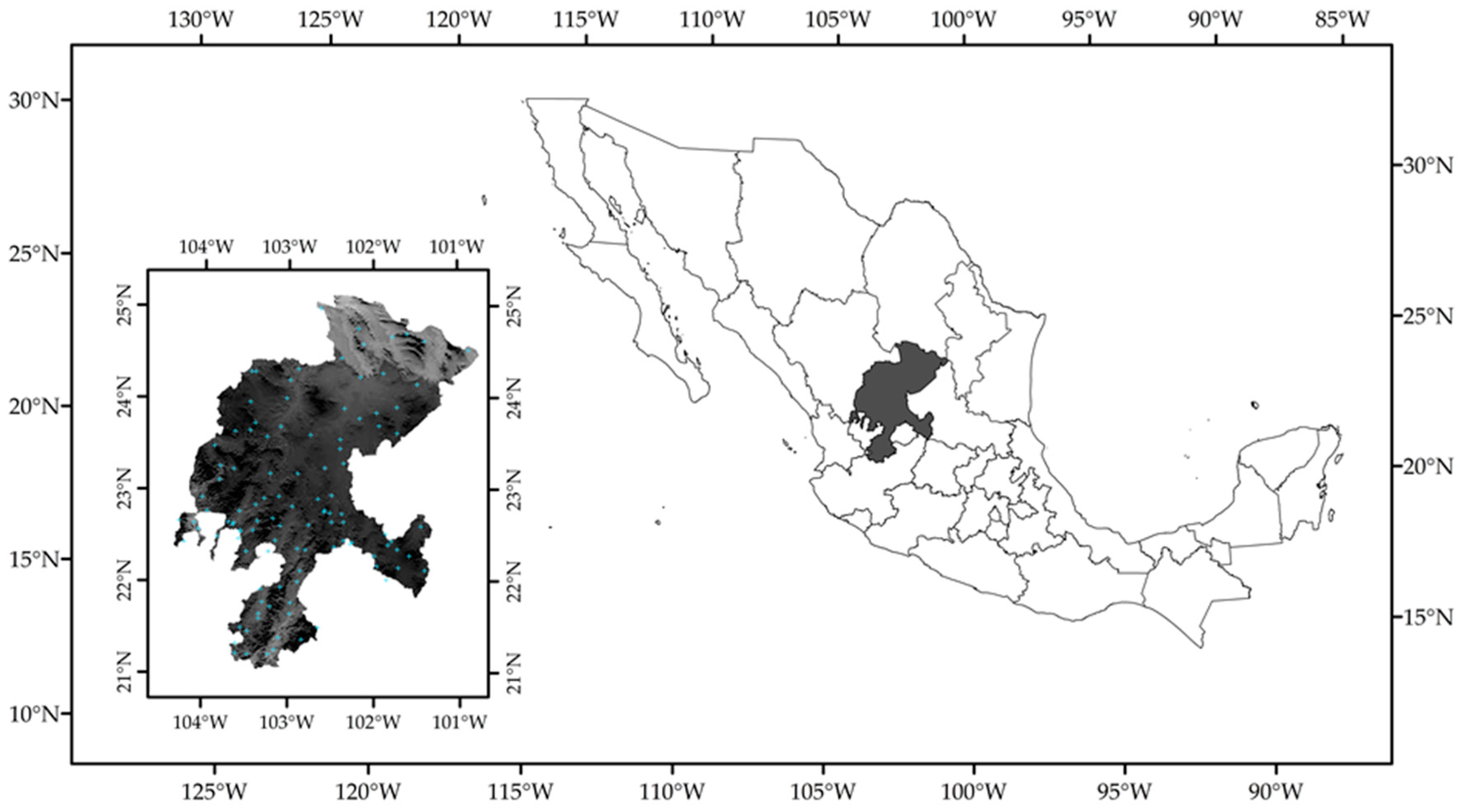
2.1. Location of Study

Zacatecas is located in the Northern region of Mexico, between extreme geographical coordinates 21°01′45.0″ N latitude and 100°43′34.3″ W longitude, and 25°07′21.5″ N latitude and 104°22′56.4″ W longitude (Figure 1). The West and Southwest of the territory is part of the Sierra Madre Occidental mountain range conformed by plateaus reaching 2850 m above sea level. The Central portion is set in the Meseta Central Highland, with valleys around 1000 m above sea level. The North is part of the Sierra Madre Oriental mountain range, with the highest elevations of the State, reaching an altitude of 3200 m above sea level [26]. Zacatecas climate is semiarid, with minimum and maximum mean monthly temperatures of 6.5 °C (January), and 29.6 °C (May), respectively. Average annual precipitation is approximately 350 mm, of which 80% occurs from June through September. A total of 1.7 Mha are devoted to agriculture, and 89% of this area is under rainfed conditions. A network composed of 111 weather stations located within the area of study was used to measure daily rainfall, and daily minimum, maximum, and average air temperature. The weather stations are monitored by the National Water Commission of the Mexican Government.

2.2. SPI and RDI Approaches

Soil moisture conditions respond to rainfall anomalies in a short time, while groundwater, runoff and reservoir storage reflect water scarcity in the mid to long term. The SPI and RDI approaches can assess water deficit using different timescales [27], and using historical records of precipitation or precipitation/potential evapotranspiration, respectively. The dataset was adjusted to the Probability Density Function (PDF) to transform raw information to standardized normal distributions. Both indexes represent the number of standard deviations separating an observation from the historical average [7], with values between −3.0 and 3.0. A negative index expresses water deficit. Drought intensity increases as the value reaches −3.0 [28]. To take into account variations in precipitation occurring among months, the incomplete Gamma distribution (Equation (1)) is the commonly used PDF to characterize the drought phenomenon [29,30].
G ( x ) = 1 Γ ( α ) 0 x t α 1 e t dt
Parameters Γ(α), α, and β are obtained as
Γ ( α ) = x α 1 e x
α = 1 4 A ( 1 + 1 + 4 3 A ) β = x ¯ α A = ln ( x ¯ ) ln ( x ) n
where α is a shape parameter (adim); β is a scale parameter (adim); n’ is the precipitation data (no zeroes); x is precipitation (mm) or precipitation/potential evapotranspiration (adim) in month i; and x ¯ is the average precipitation (mm) or the average ratio of precipitation to potential evapotranspiration (adim) in the analyzed period. For α values lower than 5.6, the shape parameter was corrected by subtracting ∆α (Equation (4)) to consider the maximum likelihood estimation of the Gamma distribution parameters [10,31].
Δ α = a 0 + a 1 α + a 2 α 2 + a 3 α 3 + a 4 α 4 + a 5 α 5
Equation (4) includes the ai coefficients, as determined by Thom [32]. Since Equation (1) is not defined for x = 0, and the dataset contains months without precipitation, Equation (5) must be used to account for zero value probability [29].
H ( x ) = q + ( 1 q ) G ( x ) ; If   x = 0 , H ( 0 ) = q
where H(x) is a cumulative probability function (adim), q is the probability of zeroes, which is determined using the relationship between the number of zeroes and the total number of data (adim), and 1 − q (adim) is the probability of values different from zero. Finally, Equation (5) is transformed into a normal distribution with a random variable Z (Equation (6)) with mean of zero and standard deviation of one [30,33].
Z = { ( t c 0 + c 1 t + c 2 t 2 1 + d 1 t + d 2 t 2 + d 3 t 3 ) for   0 < H ( x ) 0.5 ( t c 0 + c 1 t + c 2 t 2 1 + d 1 t + d 2 t 2 + d 3 t 3 ) for   0.5 < H ( x ) < 1
t = { ln ( 1 ( H ( x ) ) 2 ) for   0 < H ( x ) 0.5 ln ( 1 ( 1 H ( x ) ) 2 ) for   0.5 < H ( x ) < 1
In the estimation of SPI and RDI, x values represent cumulative precipitation or the relationship between cumulative precipitation and cumulative potential evapotranspiration in the period, respectively.

2.3. Drought Severity Assessment

Drought severity was assessed through SPI and RDI. Both indexes were computed to evaluate agricultural and hydrological drought. For each case, Z values were interpolated to obtain the quantitative magnitude of drought and the qualitative duration and frequency of drought. In this study, SPI and RDI were estimated in the initial (x) and standardized forms. The x values were calculated for the i-th year in a timescale basis of k months. Equation 8 was used to estimate the initial values of SPI.
x k ( i ) = j = 1 k P i j i = 1 ,   2 ,   3 , ,   N j = 1 ,   2 ,   3 , ,   k
The initial RDI was estimated with Equation (9). This is applicable to the estimation of RDI in both normalized (RDIn) as standardized (RDIst) forms [29,34,35]. RDIn and RDIst were obtained using Equations (10) and (11), respectively. However, Equation (11) is not defined for initial values equal to zero. For this reason, RDIst is usually calculated by fitting the Gamma PDF [15,36,37,38].
x k ( i ) = j = 1 k P i j j = 1 k PET i j i = 1 ,   2 ,   3 , ,   N j = 1 ,   2 ,   3 , ,   k
RDI n ( i ) = x k ( i ) x k ( i ) ¯ 1
RDI st ( i ) = y k ( i ) y k ( i ) ¯ σ y k ^ y k ( i ) = ln   x k ( i )
in which Pij and PETij are the precipitation and the potential evapotranspiration of the j-th month of the i-th year, and N is the total number of years in the available data set. According to Kousari et al. [15] and Zarch et al. [29] both SPI and RDI perform similar for Gamma distribution (Equations (1)–(7)), this approach solves the problem of lognormal distribution (Equation (11)) which includes zero values of precipitation. In this sense, Equation (12) express the condition of SPIst and RDIst.
Z = { SPI st If Z is estimated from Equation (8) RDI st If Z is estimated from Equation (9)
Potential evapotranspiration was estimated using the Thornthwaite method (Equation (13)) because is only based on temperature. Additionally, RDI estimation has been found to be similar when the index is computed using more sophisticated PET methodologies, such as the FAO Penman-Monteith [35,37].
PET = 16   K a ( 10 T ¯ I ) a
I = m = 1 12 ( T ¯ m 5 ) 1.514 a = 675 × 10 9   I 3 771 × 10 7   I 2 + 179 × 10 4   I + 0.492
where PET is potential evapotranspiration (mm), T ¯ is the mean temperature for the month (Celsius); Ka is a constant depending on the latitude and the month for the year (adim); and I is the temperature efficiency index (adim).
Z values for both SPI and RDI can be related to drought severity. Table 1 shows the relationship between Standardized Precipitation Index or Reconnaissance Drought Index and drought condition [39].

2.4. Software for Data Analysis and Drought Mapping

The database was assembled in a Microsoft® Excel 2016 spreadsheet. For every weather station data were filtered and chronologically sorted. Daily precipitation and reference evapotranspiration data went through a quality check to identify spurious values. Subsequently, these daily values were transformed into monthly average series. The methodology described in Equations (1)–(14) for SPI and RDI calculations was performed with a MATLAB software script. Z values were interpolated using the ordinary Kriging method due to its benefits in comparison with alternative, traditional methods. Thiessen polygons and arithmetic procedures have been reported to overestimate average rainfall [40]. Kriging interpolation is based in a mathematical multistep process, and an exploratory statistical analysis minimizes its predictive errors [41,42,43,44]. Kriging is a standard method of optimal interpolation included in ArcMap for ArcGIS® with a 0.005 output cell size.

3. Results and Discussion

A number of drought studies recognized SPI and RDI as meteorological and agricultural indexes, respectively [45]. Other authors have found that SPI for a 3 month timescale can be used to estimate agricultural droughts, while a 12-month timescale is useful to evaluate hydrological droughts [18,20,46]. Based on the monthly homogeneous precipitation and temperature dataset, SPI and RDI were mapped using 3, 6, and 12 months timescales. Producers choose a specific sowing date according to regional customs; farmers who irrigate tend to sow as early as possible to take advantage of the market (high prices for early producers). Farmers who do not irrigate wait for the best opportunity that precipitation can provide, choosing the sowing date empirically after the first significant rainfall. For rainfed crops, the sowing period usually oscillates between April and July, depending on the type of crop established and once precipitation starts [47,48]. April was selected to start the drought analysis because this is the month when farmers commonly start to establish crops in the region. Ten years of data (2005–2014) were plotted for each index. The results indicate that Zacatecas region suffers from incipient drought to severe drought in 6 or 7 years, depending of the selected timescale.
The analysis of drought parameters (magnitude, duration and frequency) did not reflect clear differences between SPI and RDI. Both indexes characterize drought condition (Table 1) with differences between them not reaching 10%. Nevertheless, our findings evidence exceptional variations among timescales with differences between SPI and RDI higher than 5 times in some cases. Figure 2 shows SPI and RDI values for 3 (April–June) and 6 (April–September) months timescales for drought years (2005 and 2011) and wet years (2007 and 2014). The eight plots present the weather in the Zacatecas territory (x-axis) through Z values (y-axis); weather stations with indexes below normal conditions (Z lower than −0.5) reflect climate anomalies to satisfy crop water requirements; the opposite happens for weather stations with indexes above normal conditions (Z higher than 0.5).
Eighty maps were produced to assess the space-time drought performance in Zacatecas from 2005 to 2014, using 3, 6, 9, and 12 months timescales. For a 3 month timescale, SPI and RDI show incipient drought in the April–June period in 2006, 2008 and 2013 (Figure 3 and Figure 4). Such indexes change to wet conditions for July–September in same years (Figure A1 and Figure A2). A quantitative analysis of drought magnitude for 3 and 6 months showed differences in the type of drought severity in less than 10% of the territory when SPI and RDI were compared; nevertheless, the difference increased for the 12 months period. In 2011, RDI (3- and 6-month timescales) was higher than SPI in 5% of the region; for 12 months the difference was about 8%. In 2014 (12 months scale) SPI analysis found 74% of territory in normal conditions, while RDI analysis only found 21% in the same drought condition, and 59% of the State was in moderate wet condition. A qualitative analysis of the information indicated similar durations and frequencies between indexes (Figure 3 and Figure 4 and Figure A1, Figure A2, Figure A3, Figure A4, Figure A5 and Figure A6). For the period studied, the duration of drought events ranged between 3 months and 3 years. In 2005 a severe drought occurred from April to June; however, normal conditions were found from July to September. However, the 12-month map indicated a dry year, extending this category to the first trimester of 2006. A drought with a duration of 3 months (July–September) was found in 2009. From April to June the conditions were categorized as wet. A 6-month drought analysis in the same year and semester (April–September) found the territory under normal conditions. The 12-month timescale revealed that parts of the region were under extreme humidity. In the period of 2005 to 2014, the longest drought event occurred from 2010 to 2012, with 2011 being the year with the most severe conditions. Exceptional drought was found at all scales (3, 6 and 12 months).
Drought estimation using a six-month timescale (April–September) and twelve-month timescale (April–March) for the abovementioned three years (2006, 2008 and 2013) show wet conditions. The corresponding drought maps are included in Appendix A: SPI and RDI for six-month and twelve-month timescale are expressed in Figure A3, Figure A4, Figure A5 and Figure A6. Due to the variations that can occur between periods, it is advisable to select the period of analysis properly. In an agricultural context, the three-month timescale is required to analyze drought severity in order to avoid underestimation of seasonal drought. The severity of drought is commonly used to express the resulting damage (Table 2). Taking into account 2005 and 2011 as drought years, Table 2 shows that, for the 3-month (April–June) timescale, around 70% of the Zacatecas territory suffered from severe to exceptional drought. Nevertheless, for the 6-month (April–September) timescale, drought conditions were apparently less severe: the Zacatecas territory changed to moderate or incipient drought, and even reached normal conditions.
The impact of drought is usually measured by assessing its effect on specific sectors (hydrological, productive, social). Table 3 presents the economic losses of the main rainfed crops (bean, corn, oats, barley, wheat, and sorghum) in the region of study. In ten years, Zacatecas has lost 478 million US dollars because of droughts. 2005, 2009, and 2011 were the most critical years, with 47%, 39%, and 63% agricultural economical losses. Conversely, 2006 and 2013 barely reached 2% and 1% losses, respectively. Such values are in agreement with drought severity estimates (Table 2): 2005 and 2011 were both dry years (drought indexes were less than −1.25 in whole territory), while 2006 and 2013 were wet years with periods of normal precipitations (drought indexes were higher than −0.05 in the whole territory).

4. Conclusions

Mexico has frequently suffered from adverse climatic conditions. While the southeastern part of the country has undergone huge floods, the Central and North portions have experienced critical droughts. Understanding drought and its patterns (frequency, duration, and severity) is particularly important in semiarid regions. Such knowledge allows us to combat the adverse effects of drought in a proactive manner, and to address the risks that drought implies. 73% of Zacatecas territory (75,284 km2) is characterized by dry climate (rainfall is lower than potential evapotranspiration). This implies significant limitations on agriculture [26], as confirmed by the drought maps presented in this article. For the period 2005–2014, regardless of the timescale or index used, large parts of the Zacatecas area ranged from normal conditions to exceptional drought during five out of ten analyzed years. Results confirmed that the 12-month time scale was the most benevolent analyzed timescale. Nevertheless, the three-month timescale [24,48] is crucial for the analysis of drought in agricultural contexts. In this sense, the reported maps identify major threats to rainfed crop production: seven out of ten analyzed years ranged from minimum wet to vast scarcity, causing economic losses in agriculture exceeding 10% in of these years. Losses reached values as high as 39%, 47%, and 63% in 2009, 2005, and 2011, respectively. As Mishra and Singh [17] stated, the importance of analyzing historical droughts lies in the generation of information related to water deficits with respect to water demands during drought periods. This allows the design of policies to meet the challenges likely to occur in case of future droughts, either for new or existing water resource projects. The mapping of drought offers a broad spatial and temporal spectrum of droughts in Zacatecas, Mexico; the eighty maps generated show how drought severity and drought duration evolve across both space and time. For a given timescale it was very common to observe that almost the entire study area suffered the same drought conditions. Nevertheless, some peculiarities arose: (1) the most frequent and severe droughts occurred in the Northern region, reaching extreme and exceptional drought conditions in some years; and (2) wet conditions occurred only in very few locations located in the Southern part of the State. The recurrence of drought in the country has prompted the Mexican Government to define stricter policies to deal with this phenomenon. In 2013, it launched a series of actions aimed at preventing and mitigating its effects; among them is the research into drought indexes and methodologies that contribute to early warning for drought [49]. Because of this, our contribution could support the management of regional drought, providing fresh information about incidence and severity of drought in Zacatecas using maps plotted trough SPI and RDI as two well-accepted indexes to evaluate agricultural drought.

Acknowledgments

To Consejo Zacatecano de Ciencia, Tecnología e Innovación of Zacatecas, Mexico, for the funds provided to the project FOMIX CONACyT, Zacatecas State Government “State Information System for the Characterization, Prevention and Mitigation of Drought”, with code ZAC-2013-C02-197731.

Author Contributions

All authors contributed to this work significantly. Carlos Bautista-Capetillo and Hugo Júnez-Ferreira contributed to the subject of research, literature review, statistical analysis of climatic data, and drought interpretation and finalized the manuscript. Brenda Carrillo and Gonzalo Picazo collected and processed climatic data and produced the drought maps.

Conflicts of Interest

The authors declare no conflict of interest.

Appendix A

Figure A1. Three-month timescale Standard Precipitation Index (July–September).
Water 08 00416 g005
Figure A2. Three-month timescale Reconnaissance Drought Index (July–September).
Water 08 00416 g006
Figure A3. Six-month timescale Standard Precipitation Index (April–September).
Water 08 00416 g007
Figure A4. Six-month timescale Reconnaissance Drought Index (April–September).
Water 08 00416 g008
Figure A5. Twelve-month timescale Standard Precipitation Index (April–March).
Water 08 00416 g009
Figure A6. Twelve-month timescale Reconnaissance Drought Index (April–March).
Water 08 00416 g010

References

  1. Coumou, D.; Rahmstorf, S. A decade of weather extremes. Nat. Clim. Chang. 2012, 2, 491–496. [Google Scholar] [CrossRef]
  2. Perevochtchikova, M.; De La Torre, J.L.L. Causas de un desastre: Inundaciones del 2007 en Tabasco, México. J. Lat. Am. Geogr. 2010, 9, 73–98. [Google Scholar] [CrossRef]
  3. Rosenzweig, C.; Iglesias, A.; Yang, X.B.; Epstein, P.R.; Chivian, E. Climate change and extreme weather events; implications for food production, plant diseases, and pests. Glob. Chang. Hum. Health 2001, 2, 90–104. [Google Scholar] [CrossRef]
  4. Flores, L.I.; Bautista-Capetillo, C. Green and blue water footprint accounting for dry beans (Phaseolus vulgaris) in primary region of Mexico. Sustainability 2015, 7, 3001–3016. [Google Scholar]
  5. Boubacar, I. The effects of drought on crop yields and yield variability: An economic assessment. Int. J. Econ. Financ. 2012, 4, 51. [Google Scholar] [CrossRef]
  6. Padilla, G.; Rodríguez, L.; Castorena, G.; Florescano, E. Análisis Histórico de las Sequías en México; Secretaría de Agricultura y Recursos Hidráulicos, Comisión del Plan Nacional Hidráulico SARH: México D.F., Mexico, 1980. [Google Scholar]
  7. Corvera, M.C. Caracterización de la sequía en el estado de Zacatecas. Master’s Thesis, Universidad Autónoma de Zacatecas, Zacatecas, Mexico, 2007. [Google Scholar]
  8. Ortega-Gaucin, D.; Velasco, I. Aspectos socioeconómicos y ambientales de las sequías en México. Aqua-LAC 2013, 5, 78–90. [Google Scholar]
  9. Centro Nacional de Prevención de Desastres (CENAPRED). Reseña Histórica de Sequías en México y Otras Partes del Mundo; Secretaría de Gobernación, Government of Mexico: México D.F., Mexico, 2002.
  10. National Drought Mitigation Center (NDMC), University of Nebraska, Lincon, NE, USA. Available online: http://drought.unl.edu (accessed on 8 February 2016).
  11. Tsakiris, G.; Nalbantis, I.; Vangelis, H.; Verbeiren, B.; Huysmans, M.; Tychon, B.; Poelmans, L. A system-based paradigm of drought analysis for operational management. Water Resour. Manag. 2013, 27, 5281–5297. [Google Scholar] [CrossRef]
  12. Wilhite, D.A. Breaking the hydro-illogical cycle: Progress or status quo for drought management in the United States. Eur. Water 2011, 34, 5–18. [Google Scholar]
  13. Velasco, I. Plan de Preparación para Afrontar Sequías en un Distrito de Riego. Ph.D. Thesis, Divisón de Estudios de Posgrado de la Facultad de Ingeniería, Campus Morelos, The National Autonomous University of Mexico (UNAM), Cuernavaca, Mexico, 2002. [Google Scholar]
  14. Buttafuoco, G.; Caloiero, T. Drought events at different timescales in southern Italy (Calabria). J. Maps 2014, 10, 529–537. [Google Scholar] [CrossRef]
  15. Kousari, M.R.; Dastorani, M.T.; Niazi, Y.; Soheili, E.; Hayatzadeh, M.; Chezgi, J. Trend detection of drought in arid and semi-arid regions of Iran based on implementation of reconnaissance drought index (RDI) and application of non-parametrical statistical method. Water Resour. Manag. 2014, 28, 1857–1872. [Google Scholar] [CrossRef]
  16. Trambauer, P.; Maskey, S.; Werner, M.; Pappenberger, F.; Van Beek, L.P.H.; Uhlenbrook, S. Identification and simulation of space-time variability of past hydrological drought events in the Limpopo River basin, southern Africa. Hydrol. Earth Syst. Sci. 2014, 18, 2925–2942. [Google Scholar] [CrossRef]
  17. Mishra, A.K.; Singh, V.P. A review of drought concepts. J. Hydrol. 2010, 391, 202–216. [Google Scholar] [CrossRef]
  18. Vicente-Serrano, S.M.; Cuadrat-Prats, J.M.; Romo, A. Early prediction of crop production using drought indices at different time-scales and remote sensing data: Application in the Ebro Valley (North-East Spain). Int. J. Remote Sens. 2006, 27, 511–518. [Google Scholar] [CrossRef]
  19. Tsakiris, G.; Vangelis, H. Establishing a drought index incorporating evapotranspiration. Eur. Water 2005, 9, 3–11. [Google Scholar]
  20. Elagib, N.A. Meteorological drought and crop yield in sub-Saharan Sudan I. Int. J. Water Resour. Arid Environ. 2013, 2, 164–171. [Google Scholar]
  21. Tsakiris, G.; Vangelis, H.; Tigkas, D. Drought impacts on yield potential in rainfed agriculture. In Economics of Drought and Drought Preparedness in a Climate Change Context; López-Francos, A., Ed.; CIHEAM/FAO/ICARDA/GDAR/CEIGRAM/MARM: Zaragoza, Spain, 2010; Volume 95, pp. 191–197. [Google Scholar]
  22. Spinoni, J.; Naumann, G.; Vogt, J.V.; Barbosa, P. The biggest drought events in Europe from 1950 to 2012. J. Hydrol. Reg. Stud. 2015, 3, 509–524. [Google Scholar] [CrossRef]
  23. Naumann, G.; Spinoni, J.; Vogt, J.V.; Barbosa, P. Assessment of drought damages and their uncertainties in Europe. Environ. Res. Lett. 2015, 10, 1–14. [Google Scholar] [CrossRef]
  24. Jayasree, V.; Venkatesh, B. Analysis of rainfall in assessing the drought in semi-arid region of Karnataka State, India. Water Resour. Manag. 2015, 29, 5613–5630. [Google Scholar] [CrossRef]
  25. Historical Database of Precipitation and Temperature; Comisión Nacional del Agua (CONAGUA), Government of Mexico: México D.F., Mexico, 2015.
  26. Instituto Nacional de Estadística y Geoegrafía (INEGI). Información del Territorio Nacional por Entidad. Government of Mexico. Available online: http://cuentame.inegi.org.mx/monografias/informacion/zac/ (accessed on 4 July 2016).
  27. Martínez, D. Impacto de las Sequías en el Estado de Sinaloa dentro de la Actividad Agrícola y Ganadera. Master’s Thesis, Divisón de Estudios de Posgrado de la Facultad de Ingeniería, The National Autonomous University of Mexico (UNAM), México D.F., Mexico, 2006. [Google Scholar]
  28. Crespo, P.G. Comparación de dos Metodologías para el Cálculo de la Severidad de Sequía para Doce Reservas de la Biósfera Mexicana; UNESCO: Texcoco, Mexico, 2005. [Google Scholar]
  29. Zarch, M.A.A.; Sivakumar, B.; Sharma, A. Droughts in a warming climate: A global assessment of Standardized Precipitation Index (SPI) and Reconnaissance Drought Index (RDI). J. Hydrol. 2015, 526, 183–195. [Google Scholar] [CrossRef]
  30. McKee, T.B.; Doeskin, N.J.; Kleist, J. The relationship of drought frequency and duration to time scales. In Proceedings of the 8th Conference on Applied Climatology, Anaheim, CA, USA, 17–22 January 1993; pp. 179–184.
  31. Campos-Aranda, D.F. Comparación de tres métodos estadísticos para detección y monitoreo de Sequías meteorológicas. Agrociencia 2014, 48, 463–476. [Google Scholar]
  32. Thom, H.C.S. Same Methods of Climatological Analyses; World Meteorological Organization: Geneva, Switzerland, 1966. [Google Scholar]
  33. Abramowitz, M.; Stegun, I. Handbook of Mathematical Functions with Formulas, Graphs, and Mathematical Tables; Dover Publications Inc.: New York, NY, USA, 1970. [Google Scholar]
  34. Tigkas, D.; Vangelis, H.; Tsakiris, G. The RDI as a composite climatic index. Eur. Water 2013, 41, 17–22. [Google Scholar]
  35. Tsakiris, G.; Nalbantis, I.; Pangalou, D.; Tigkas, D.; Vangelis, H. Drought meteorological monitoring network design for the reconnaissance drought index (RDI). In Drought Management: Scientific and Technological Innovations; López-Francos, A., Ed.; Centre International de Hautes Etudes Agronomiques Méditerranéennes (CIHEAM): Zaragoza, Spain, 2008; Volume 80, pp. 57–62. [Google Scholar]
  36. Mosaedi, A.; Zare Abyaneh, H.; Ghabaei Sough, M.; Samadi, S.Z. Quantifying changes in reconnaissance drought index using equiprobability transformation function. Water Resour. Manag. 2015, 29, 2451–2469. [Google Scholar] [CrossRef]
  37. Vangelis, H.; Tigkas, D.; Tsakiris, G. The effect of PET method on Reconnaissance Drought Index (RDI) calculation. J. Arid Environ. 2013, 88, 130–140. [Google Scholar] [CrossRef]
  38. Zarch, M.A.A.; Malekinezhad, H.; Mobin, M.H.; Dastorani, M.T.; Kousari, M.R. Drought monitoring by reconnaissance drought index (RDI) in Iran. Water Resour. Manag. 2011, 25, 3485–3504. [Google Scholar] [CrossRef]
  39. Svoboda, M.; LeComte, D.; Hayes, M.; Heim, R.; Gleason, K.; Angel, J.; Rippey, B.; Tinker, R.; Palecki, M.; Stooksbury, D.; et al. The drought monitor. Bull. Am. Meteorol. Soc. 2002, 83, 1181–1190. [Google Scholar]
  40. Íñiguez, M.; Ojeda, W.; Díaz, C.; Mamadou Bâ, K.; Mercado, R. Análisis metodológico de la distribución espacial de la precipitación y la estimación media diaria. Rev. Mex. Cienc. Agríc. 2011, 2, 57–69. [Google Scholar]
  41. Viera, M.A.D. Geoestadística Aplicada; Instituto de Geofísica, Universidad Nacional Autónoma de México, Ministerio de Ciencia, Tecnología y Medio Ambiente de Cuba: México D.F., Mexico, 2002; pp. 31–57. [Google Scholar]
  42. ArcGIS PRO. Available online: https://pro.arcgis.com/en/pro-app/tool-reference/3d-analyst/ (accessed on 16 August 2016).
  43. Bohling, G. Kriging. Kansas Geological Survey, Technical Report. 2005. Available online: http://people.ku.edu/~gbohling/cpe940 (accessed on 16 August 2016).
  44. Oliver, M.A.; Webster, R. Kriging: A method of interpolation for geographical information systems. Int. J. Geogr. Inf. Syst. 1990, 4, 313–332. [Google Scholar] [CrossRef]
  45. Pedro-Monzonís, M.; Solera, A.; Ferrer, J.; Estrela, T.; Paredes-Arquiola, J. A review of water scarcity and drought indexes in water resources planning and management. J. Hydrol. 2015, 527, 482–493. [Google Scholar] [CrossRef]
  46. Hurtado, G.M. Cadena, Aplicación de índices de sequía en Colombia. Meteorol. Colomb. 2002, 5, 131–137. [Google Scholar]
  47. Luna, M. Antología Cultivos Básicos en Zacatecas; Universidad Autónoma de Zacatecas: Zacatecas, Mexico, 2014; Available online: https://www.academia.edu/11532162/ (accessed on 16 August 2016).
  48. Medina, G.; Rumayor, R.; Cabañas, C.; Luna, F.; Ruiz, C.; Gallegos, V.; Madero, J.; Gutiérrez, R.; Rubio, S.; Bravo, L. Potencial Productivo de Especies Agrícolas en el Estado de Zacatecas; Instituto Nacional de Investigaciones Forestales, Agrícolas y Pecuarias, Centro de Investigación Regional Norte Centro: Calera, Zacatecas, Mexico, 2003. [Google Scholar]
  49. Comisión Nacional del Agua (CONAGUA). Política Pública Nacional para la Sequía; Programa Nacional contra la Sequía, Government of Mexico: México D.F., Mexico, 2014.
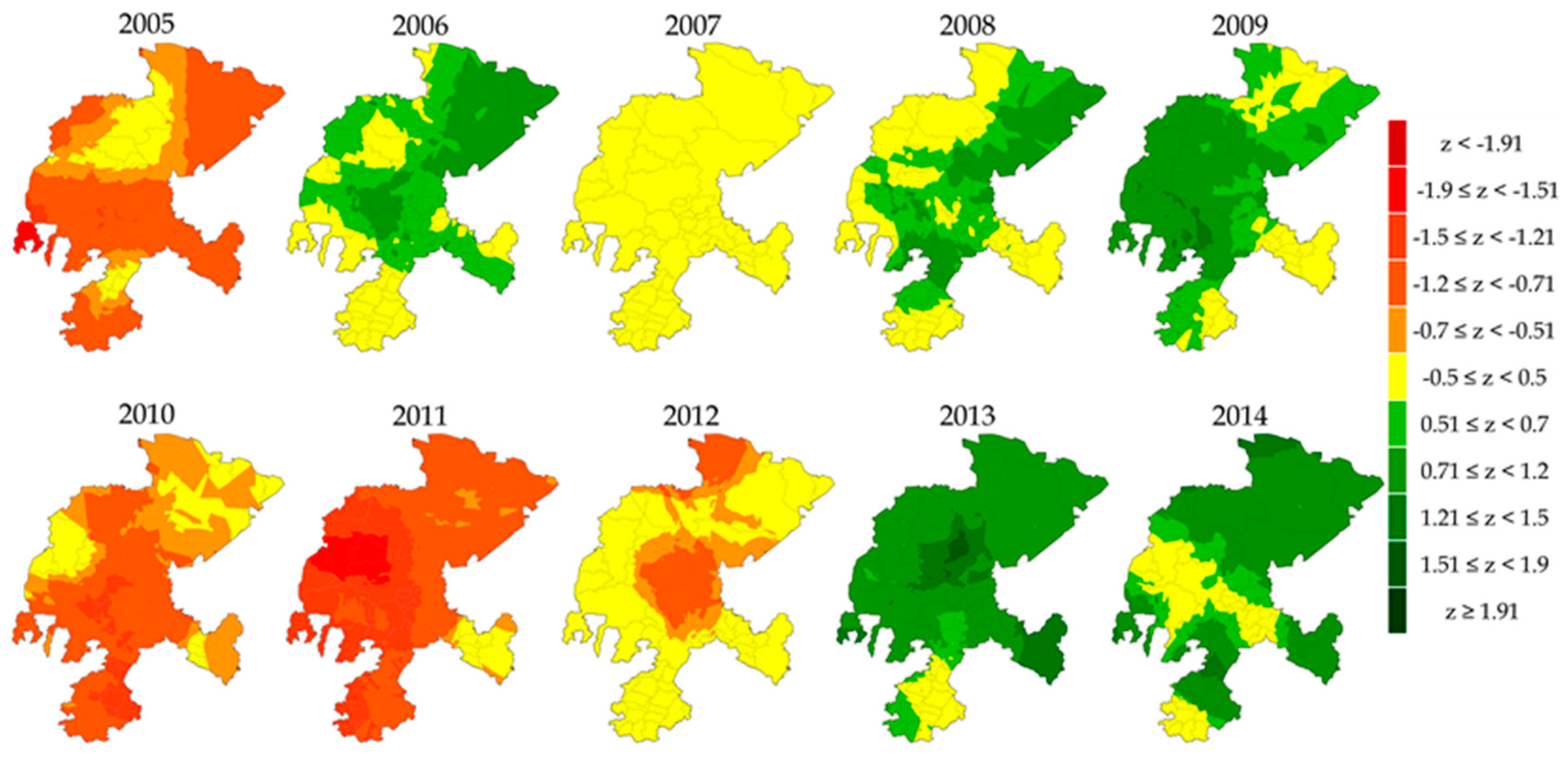
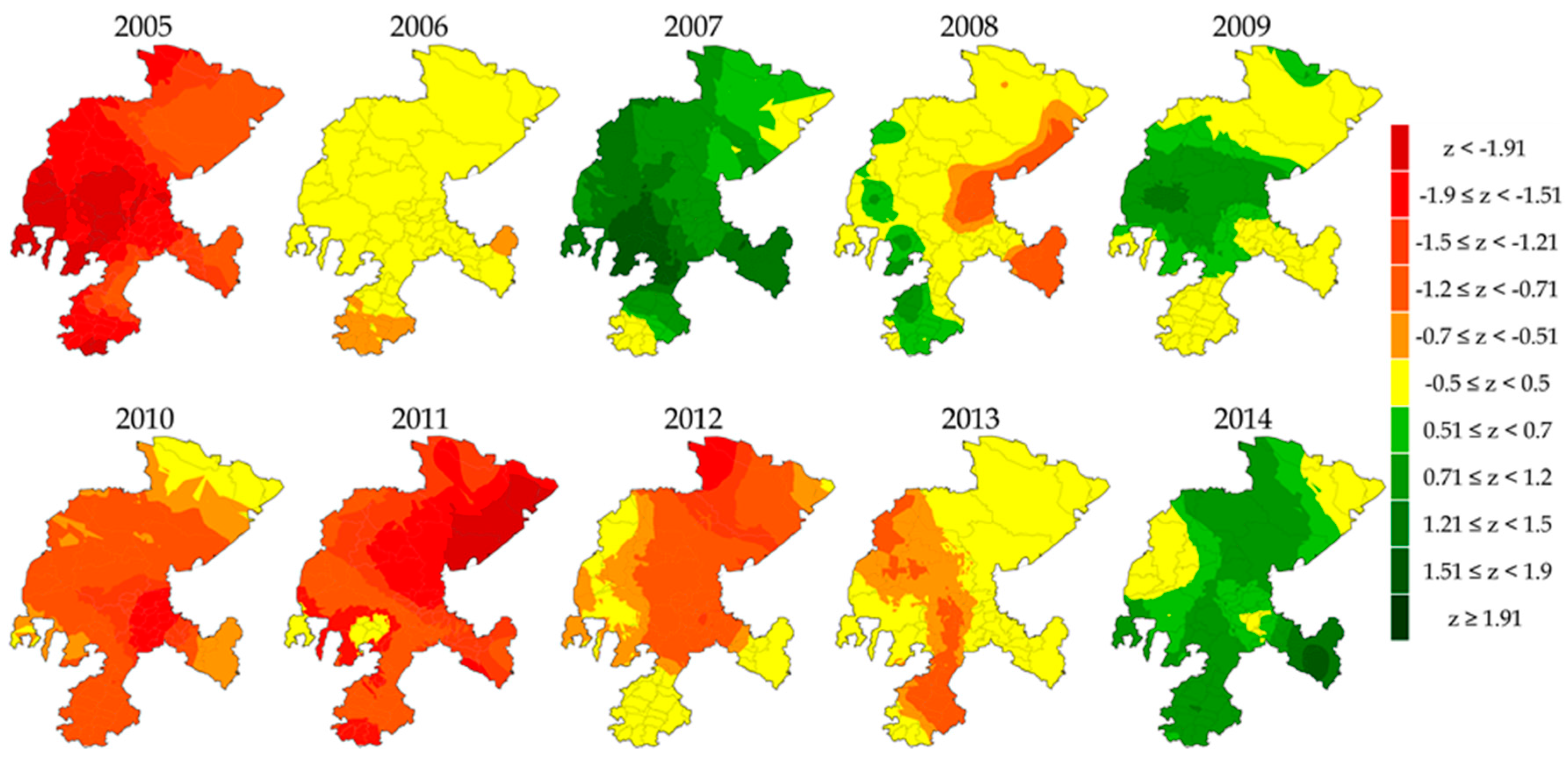
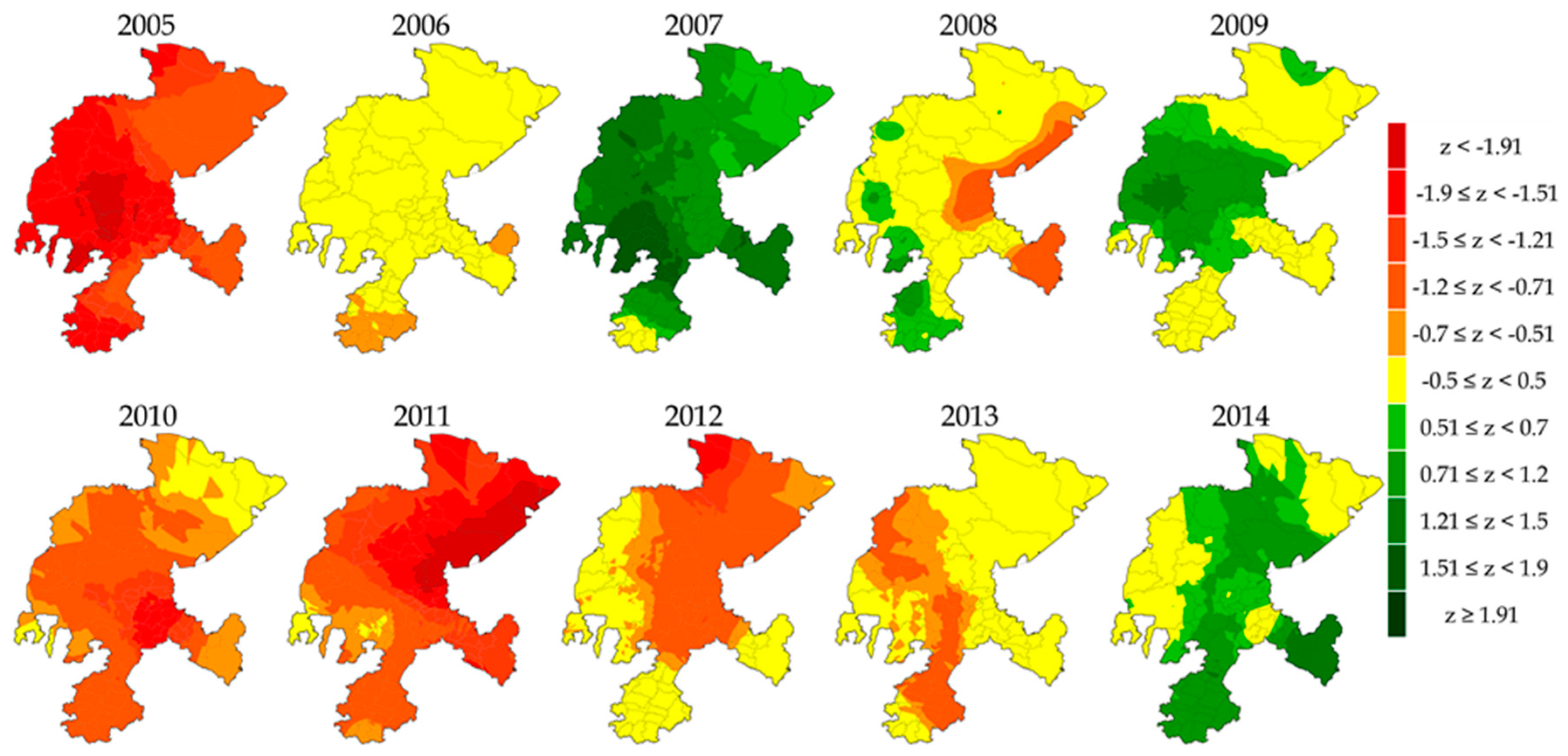
Figure 1. Geographical location of Zacatecas, Mexico. Blue dots represent weather stations.
Water 08 00416 g001
Figure 2. SPI and RDI values for all weather stations in 2005, 2007, 2011 and 2014: (a) 3 months (April–June) timescale; (b) 6 months (April–September) timescale.
Water 08 00416 g002
Figure 3. Three-month timescale Standard Precipitation Index (April–June).
Water 08 00416 g003
Figure 4. Three-month timescale Reconnaissance Drought Index (April–June).
Water 08 00416 g004
Table 1. Z values vs. drought condition (applicable to both Standardized Precipitation Index and Reconnaissance Drought Index).
Index ValueCondition
Z < −1.91Exceptional drought
−1.90 < Z ≤ −1.51Extreme drought
−1.50 < Z ≤ −1.21Severe drought
−1.20 < Z ≤ −0.71Moderate drought
−0.70 < Z ≤ −0.51Incipient drought
−0.50 < Z ≤ 0.51Normal conditions
0.51 < Z ≤ 0.70Incipient wet
0.71 < Z ≤ 1.20Moderate wet
1.21 < Z ≤ 1.50Very wet
1.51 < Z ≤ 1.90Extreme wet
1.91 < ZExceptional wet
Table 2. Percent of Zacatecas territory exposed to different drought conditions in 2005, 2007, 2011, and 2014.
YearIndexTimescale (Months)PeriodExceptional DroughtExtreme DroughtSevere DroughtModerate DroughtIncipient DroughtNormal ConditionsIncipient WetModerate WetVery WetExtreme WetExceptional Wet
2005SPI3April–June21341927
July–September 1187
RDIApril–June8401932
July–September 891
SPI6April–September 513512
RDI 443520
SPI12April–March 601918
RDI 612015
2007SPI3April–June 918352810
July–September 5886
RDIApril–June 18353410
July–September 927
SPI6April–September 44479
RDI 244926
SPI12April–March 97
RDI 100
2011SPI3April–June122325279
July–September 8431139
RDIApril–June142126288
July–September 1041841
SPI6April–September 113652
RDI 163646
SPI12April–March 82560 6
RDI 83251 6
2014SPI3April–June 2024495
July–September 51077
RDIApril–June 3524356
July–September 9871
SPI6April–September 77108
RDI 661614
SPI12April–March 74167
RDI 211559
Table 3. Comparison between drought severity and agricultural economic losses.
YearSownHarvestedSinisteredEconomic Losses (%)
MhaM$MhaM$MhaM$
20051.05980.55520.504647
20061.102001.081970.0232
20071.111450.901170.212819
20081.102630.992430.11208
20091.103590.652190.4214039
20101.101750.871380.233721
20110.931970.35740.5812363
20121.013020.832500.175221
20131.102891.082860.0231
20141.022460.922200.102611

