Article

Daily Runoff Forecasting Model Based on ANN and Data Preprocessing Techniques

1
State Key Laboratory of Water Resources and Hydropower Engineering Science, Wuhan University, Wuhan 430072, China
2
China Yangtze Power Co., Ltd., Yichang, Hubei 443002, China
*
Author to whom correspondence should be addressed.
Water 2015, 7(8), 4144-4160; https://doi.org/10.3390/w7084144
Submission received: 10 June 2015 / Revised: 17 July 2015 / Accepted: 20 July 2015 / Published: 28 July 2015
(This article belongs to the Special Issue Use of Meta-Heuristic Techniques in Rainfall-Runoff Modelling)

Abstract

:
There are many models that have been used to simulate the rainfall-runoff relationship. The artificial neural network (ANN) model was selected to investigate an approach of improving daily runoff forecasting accuracy in terms of data preprocessing. Singular spectrum analysis (SSA) as one data preprocessing technique was adopted to deal with the model inputs and the SSA-ANN model was developed. The proposed model was compared with the original ANN model without data preprocessing and a nonlinear perturbation model (NLPM) based on ANN, i.e., the NLPM-ANN model. Eight watersheds were selected for calibrating and testing these models. Comparative study shows that the learning and training ability of ANN models can be improved by SSA and NLPM techniques significantly, and the performance of the SSA-ANN model is much better than the NLPM-ANN model, with high foresting accuracy. The SSA-ANN1 model, which only considers rainfall as model input, was compared with the SSA-ANN2 model, which considers both rainfall and previous runoff as model inputs. It is shown that the Nash-Sutcliffe criterion of the SSA-ANN2 model is much higher than that of the SSA-ANN1 model, which means that the proper selection of previous runoff data as rainfall-runoff model inputs can significantly improve model performance since they usually are highly auto-correlated.

1. Introduction

Real-time hydrological forecasting plays an important role in flood control and reservoir operation, and higher forecasting precision can increase the utilization efficiency of water resources. Traditionally, hydrological simulation modeling systems are classified into three main groups, namely empirical black box, lumped conceptual, and distributed physically-based models [1]. The last two groups focus on understanding hydrological processes and involve various physical phenomena. Owing to the complexity of the rainfall-runoff process, these physical process simulations and model calibrations require large amounts of hydrological data. On the contrary, black-box modeling does not require a deep knowledge of the underlying physics and also can solve the problem of the scarcity of the data. Several black-box models have been developed and used in hydrological forecasting, such as fuzzy theory [2,3], artificial neural network [4,5], chaos [6], genetic programming [7], support vector machine [8], and so on.
Artificial neural network, inspired by research into the biological neural networks, has a flexible structure, and self-learning and self-adaptive features. In 2000, the American Society of Civil Engineering (ASCE) Task Committee explicitly reviewed the application of artificial neural networks in hydrology [9,10]. Hsu et al. [5] mentioned that the artificial neural network (ANN) model can identify the complex nonlinear relationship between runoff and rainfall time series, even though the model structure and parameters cannot represent the physical process of the catchments. Maier and Dandy [11] reviewed using ANN models to deal with water resource variables prediction, outlined the steps that should be followed in the development of ANN models, and concluded that the ANN model has advantages in hydrological forecasting. Currently, ANN is still a research hot point and has been successfully applied in hydrological forecasting [12,13,14,15,16,17,18,19,20,21,22].
Due to the highly seasonal variation, and nonlinear and noisy characteristics of hydrological time series, preprocessing input data becomes an effective way to improve model precision [23,24,25,26,27,28]. Considering the highly seasonal variation of rainfall and runoff time series, Nash and Brasi [23] developed the linear perturbation model (LPM) based on the assumption that subtraction of the seasonal means from the original series would remove much of the non-linearity of the rainfall-runoff process. The relationship between the departures is simulated by the linear response function, but only part of the nonlinearity of the rainfall-runoff process can be removed by subtracting the seasonal means. Pang et al. [16] used the ANN model to replace the linear response function and proposed a nonlinear perturbation model (NLPM) based on ANN (NLPM-ANN). The advantage of the NLPM-ANN model is that it is capable of obtaining satisfactory results even if the explicit form of the relationship between the involved variables is unknown.
Considering that the hydrological time series can be viewed as a combination of quasi-periodic signals contaminated by noises to some extent [29], the singular spectrum analysis (SSA) proposed by Vautard et al. [30] can decompose the time series into a sum of a small number of interpretable components, such as a slowly varying trend, oscillatory components, and a “structureless” noise [31]. By performing a spectrum analysis on the input data, eliminating the noises, and inverting the remaining components to yield a “filtered” time series, the model performance could be improved. Sivapragasam et al. [25] proposed a prediction technique based on SSA coupled with support vector machines to predict runoff and rainfall, and showed that the proposed technique yields a significantly higher prediction accuracy than that of the nonlinear prediction method. Wu and Chau [29] also found that SSA can considerably improve the performance of the rainfall-runoff model and it is promising in hydrological forecasting.
In this paper, an approach of improving daily runoff forecasting accuracy in terms of data preprocessing and the selection of predictive factors is discussed. The artificial neural network (ANN) is used for rainfall-runoff simulation. The SSA and LPM techniques are adopted to deal with data preprocessing. Then SSA-ANN models are developed and compared with the NLPM-ANN model based on the daily data from the eight watersheds used by Pang et al. [16]. A comparative study is also conducted involving two different types of model inputs, namely considering rainfall as an input and considering both rainfall and runoff as inputs.

2. Data-Driven Models

2.1. NLPM-ANN Model

The structure of the NLPM-ANN model as shown in Figure 1 was proposed by Pang et al. [16] to consider the influence of seasonal changes and the nonlinearity of the rainfall-runoff process. The model input is divided into two parts. The first is the series of the seasonal expectations of the input (pd) that is transformed to the series of the seasonal expectations of the output (qd) through an undefined relation. The second part, which is the input perturbations (Pi-pd), is transformed into the output perturbations (Qi-qd) through ANN. The total output is the sum of the seasonal expectations of the output and the output perturbations.
Figure 1. Schematic diagram of the NLPM-ANN model.
Water 07 04144 g001

2.2. Singular Spectrum Analysis

Singular spectrum analysis (SSA) is a suitable analysis method for researching the period oscillatory behavior. It is also a statistical technique starting from a dynamic reconstruction of the time series and is associated with empirical orthogonal function (EOF). Generally, SSA can be considered as a special application of EOF decomposition. The main purpose of SSA is converting a one-dimensional time series into a multi-dimensional matrix with a given window length, and then the orthogonal decomposition of this matrix is obtained. If the obvious pairs of eigenvalues are produced and the corresponding EOF is almost periodic or orthogonal, this corresponding EOF can be considered the oscillatory behavior of the time series.
Brief operating procedures of SSA are summarized as follows. Assume that the series is a nonzero series F = {f0, f1, …, fN−1} (fi ≠ 0), the length of series is N (>2). Given a window length L, the one-dimensional time series can be transferred into a sequence of L-dimensional vectors Xi = {fi−1, …, fi+L−2}T, (I = 1, …, K = NL+1). The K vectors Xi will form the columns of the (L × K) trajectory matrix:
X = [ f 0 f 1 f 2 f K 1 f 1 f 2 f 3 f K f 2 f 3 f 4 f K + 1 f L 1 f L f L + 1 f N 1 ]
Then the singular value decomposition (SVD) of the trajectory matrix X is conducted. Let S = XXT. The eigenvalues and eigenvectors of S can be calculated, and these eigenvalues range in the decreasing order of magnitude. According to the conventional computation of EOF, an expansion of the matrix X is represented as:
x i + j = k = 1 L a i k E j k
where i = 1, 2,…, NL + 1, j = 1,2, …, L, k = 1, 2,…, L, a i k is the time principal components (T-PC), E j k is the corresponding eigenvector denoted by T-EOF. The key step of SSA is to reconstruct a new one-dimensional series of length N using each component of the T-PC and T-EOF. The formula is expressed as follows:
x i k = { 1 i j = 1 L a i j k E j k 1 i L - 1 1 L j = 1 L a i j k E j k L i N L + 1 1 N i + 1 j = i N + L L a i j k E i j k N L + 2 i N
Equation (3) produces an N-length time series Fk, thus the initial series F is decomposed into the sum of L series:
F = k = 1 L F k
If the number of contributing components is p, then the filtered series is the sum of p series:
F = k = 1 p F k
The sum of the remaining series is noise. As mentioned above, these reconstructed components can be associated with the trend, oscillations, or noise of the original time series with proper choices of L and p.

2.3. Artificial Neural Network

ANN can be categorized as single-layer, bilayer, and multilayer according to the number of layers, and as feed-forward, recurrent, and self-organizing according to the direction of information flow and processing [9]. Among these different architectures, the multilayer feed-forward networks, which consist of an input layer, several hidden layers, and an output layer, have been widely used. Each layer has different nodes, and the number of hidden layers and the hidden nodes of each hidden layer are usually determined by trial-and-error method.
Assuming the three-layer ANN denoted by m × h × 1, where m stands for the number of input nodes, namely the number of predictive factors, and h is the number of nodes in the hidden layer, the ANN prediction model can be formulated as:
Q t + T ^ = f ( X t , w , θ , m , h ) = θ 0 + j = 1 h w j o u t φ ( i = 1 m w j i X t + θ j )
where Xt is the input data; T is the length of lead time; φ denotes transfer functions; wji are the weights defining the link between the ith node of the input layer and the jth of the hidden layer; θj are biases associated with the jth node of the hidden layer; w j o u t are the weights associated with the connection between the jth node of the hidden layer and the node of the output layer; and θ0 is the bias at the output node. The Levenberg–Marquardt algorithm is chosen to adjust the values of w and θ in this study [32].

2.4. Proposed SSA-ANN Models

The SSA-ANN models are proposed with the aim of analyzing the effect of data processing. The flowchart of SSA-ANN models is illustrated in Figure 2, where the original series is decomposed into oscillations and noise by SSA, firstly. Then the reconstructed series is selected as the ANN model input. If the input is the rainfall data series only, the SSA-ANN1 model is built to simulate the relationship between rainfall and runoff. If the input contains both the rainfall and runoff data series, the SSA-ANN2 model is built to simulate the relationship between rainfall and previous runoff with forecasting runoff.
Figure 2. Schematic diagram of SSA-ANN models.
Water 07 04144 g002

2.5. Evaluation of Model Performances

Two criteria are selected to evaluate the prediction performance based on Chinese Hydrological Forecasting (or prediction) guidelines (2008), they are:
(1)
Determination coefficient (or Nash-Sutcliffe criterion) (R2)
R 2 = ( 1 t = 1 n ( Q t Q t ) 2 t = 1 n ( Q t Q t ¯ ) 2 )
(2)
Water balance coefficient (WB)
W B = t = 1 n Q t t = 1 n Q t
where n is the number of year, Q t and Q t are the observed and forecasted inflows, respectively, Q t ¯ is the average value of observed flow; if the values of R2 and WB are closer to one, the better the prediction results that are obtained.

3. Comparative Study

3.1. Data

To compare the proposed SSA-ANN models with the NLPM-ANN model, eight watersheds in China used by Pang et al. [16] were selected as case studies in this paper. The data include the daily rainfall and runoff data. Each of data series is divided into three parts, i.e., training set, cross-validation set, and testing set. The training set is used to train the network and the cross-validation set is used to check the progress of the network and implement an early stopping approach in order to avoid the over-fitting of the training set. The testing set serves as model evaluation. Table 1 lists statistical information about all watersheds, including mean (μ), standard deviation (Sx), maximum (Xmax), and minimum (Xmin). As shown in Table 1, the training data does not cover the cross-validation or testing data totally. In order to ensure the extrapolation ability of ANN and avoid numerical difficulties during calculation, all data are scaled to the interval [−0.9, 0.9] by normalization.
Table 1. List of the watershed statistical information.
Watershed and DatasetsStatistical ParametersData Period
μSxXmaxXmin
Jiahe area: 5578 km2rainfall (mm)whole data2.35.971.40January 1980–December 1990
training data2.36.068.90
cross-validation data2.36.271.40
testing data2.15.344.20
runoff (m3)whole data58.7125.126206.5
training data61.9141.626206.5
cross-validation data55.399.612207.9
testing data50.776.4108010.1
Laoguanhe area: 4217 km2rainfall (mm)whole data2.26.469.40January 1980–December 1990
training data2.36.869.20
cross-validation data2.05.856.00
testing data2.05.769.40
runoff (m3)whole data27.173.614600.1
training data33.584.114600.4
cross-validation data16.850.65860.1
testing data14.846.17930.2
Baohe area: 3415 km2rainfall (mm)whole data2.56.980.60January 1980–December 1990
training data2.57.180.60
cross-validation data2.26.051.30
testing data2.66.880.50
runoff (m3)whole data46.5129.440200
training data49.7150.740201.2
cross-validation data31.454.85233.8
testing data50.396.820100.0
Mumahe area: 1224 km2rainfall (mm)whole data3.28.8132.80January 1980–December 1990
training data3.28.6132.80
cross-validation data3.39.398.60
testing data2.99.194.40
runoff (m3)whole data39.380.312701.2
training data41.080.812701.2
cross-validation data40.682.17964.6
testing data32.176.49902
Nianyushan area: 924 km2rainfall (mm)whole data3.811.6269.50January 1975–December 1999
training data3.912.2269.50
cross-validation data3.39.3102.50
testing data3.710.8144.70
runoff (m3)whole data18.562.120950
training data19.868.320950
cross-validation data13.533.25080
testing data17.655.98220
Gaoguan area: 303 km2rainfall (mm)whole data4.212.5179.10January 1984–December 1999
training data4.412.8179.10
cross-validation data3.511.3143.80
testing data4.212.7116.00
runoff (m3)whole data5.815.12460
training data5.714.22370
cross-validation data5.113.52460
testing data7.720.52140
Shimen area: 271.25 km2rainfall (mm)whole data3.811.4141.30January 1989–December 1999
training data3.510.1114.90
cross-validation data5.115.1141.30
testing data3.811.8116.80
runoff (m3)whole data4.915.22960
training data3.79.91500
cross-validation data8.725.12960
testing data5.517.91720
Tiantang area: 220 km2rainfall (mm)whole data3.712.1193.40January 1973–December 1984
training data3.611.6175.00
cross-validation data3.711.4151.70
testing data4.214.7193.40
runoff (m3)whole data6.118.45350
training data5.616.54000
cross-validation data5.616.53780.3
testing data8.225.65350.3

3.2. Determination of Model Inputs

The suitable predictive factors have an important impact on model performance. If the model input is only rainfall, it can be expressed as:
y i = f ( x i , x i 1 , , x i n + 1 )
where x is the rainfall series, y is the runoff series, and n is the number of antecedent rainfall components. In Pang et al.’s paper [16], only rainfall was selected as model input, so the SSA-ANN1 model, which only uses rainfall as model input, was developed. In order to ensure the comparability of model performance, the same n values for the SSA-ANN1 model and the NLPM-ANN model were selected. From Pang et al.’s results of the NLPM-ANN model [16], the values of n are 8, 6, 6, 8, 10, 8, 6, and 10 for Jiahe, Laoguanhe, Baohe, Mumahe, Nianyushan, Gaoguan, Shimen, and Tiantang, respectively.
As we know, the autocorrelation of the runoff series is strong and the impact of previous runoff on current runoff cannot be ignored, so the SSA-ANN2 model which uses rainfall and runoff as model inputs was developed in this paper. It can be expressed as:
y i = f ( y i 1 , , y i m + 1 , x i , x i 1 , , x i n + 1 )
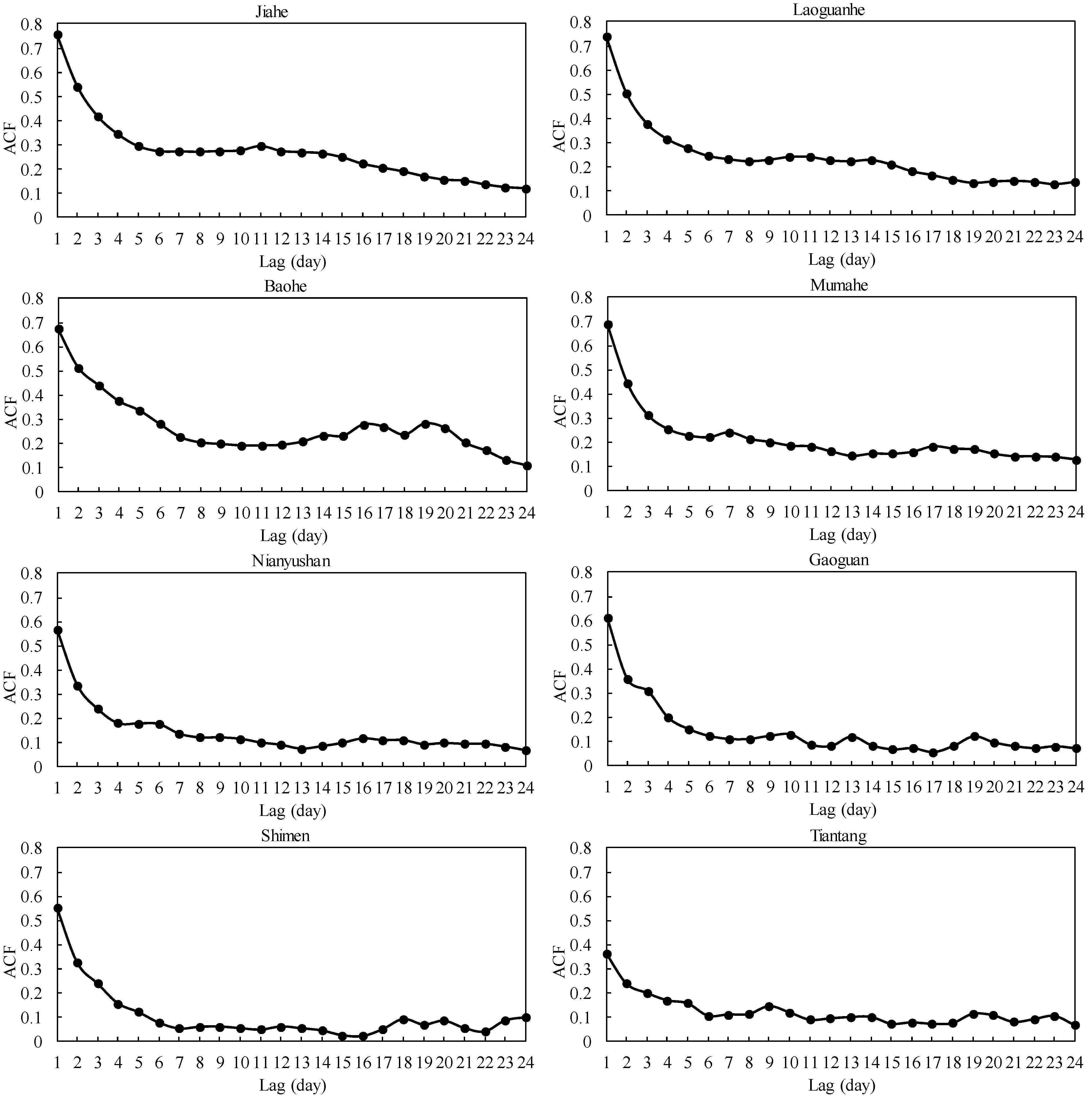
where m is the number of previous runoff data. The values of n for the SSA-ANN2 model are the same as the SSA-ANN1 model. In view of the convenience of operation and simplicity of computation, the autocorrelation function (ACF) is used to determine m. The smaller the values of correlation, the poorer the relationship is. Figure 3 plots the ACF values of the runoff series at the one-step prediction horizon. Then the number of model inputs can be taken with the values of 5, 5, 5, 3, 2, 3, 2, and 1 for Jiahe, Laoguanhe, Baohe, Mumahe, Nianyushan, Gaoguan, Shimen, and Tiantang, respectively. It can be seen that the number of previous daily runoff is obviously related with the watershed area.
Figure 3. Autocorrelation function (ACF) values of runoff series for all watersheds.
Water 07 04144 g003

3.3. Data Preprocessing

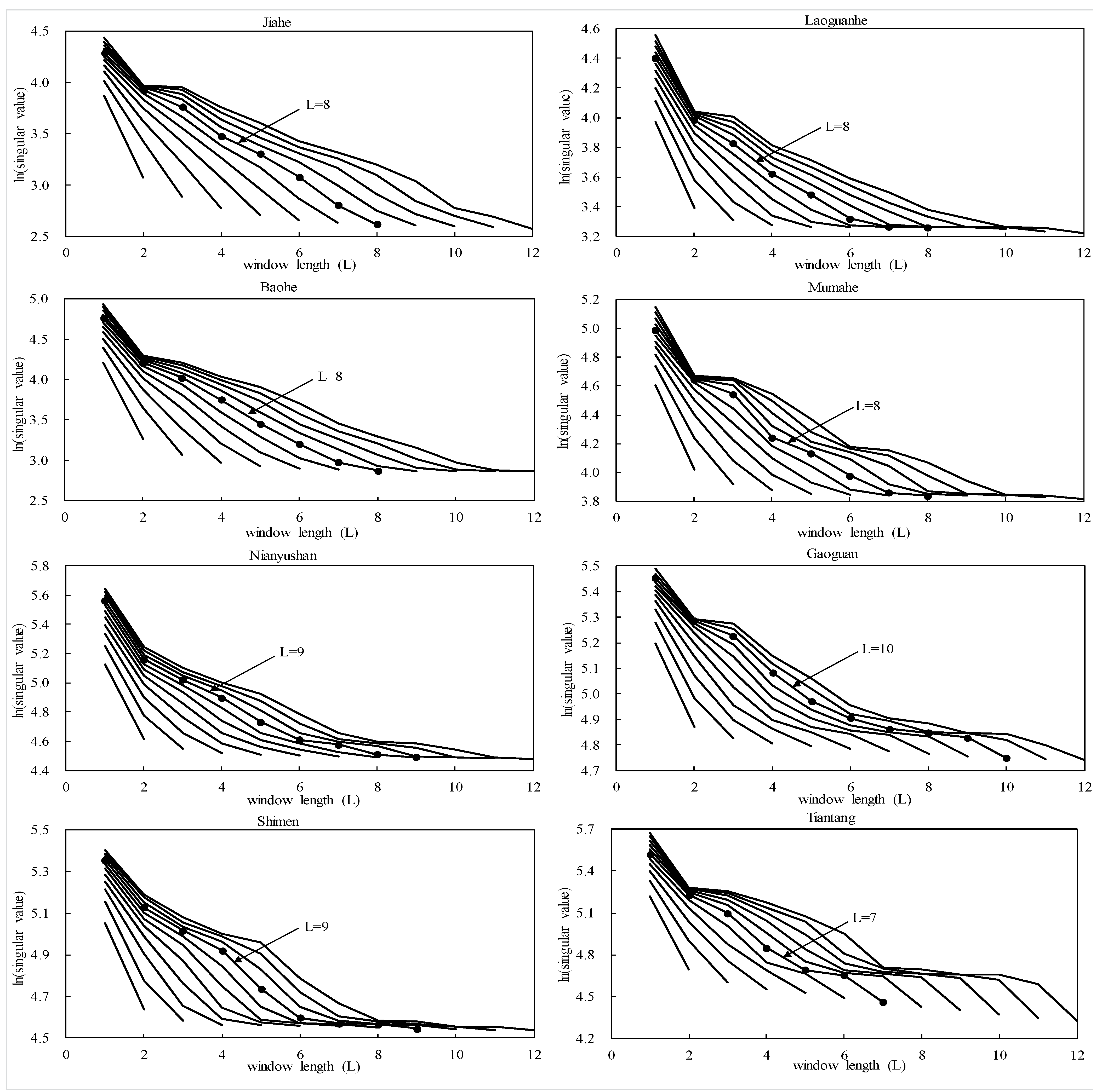
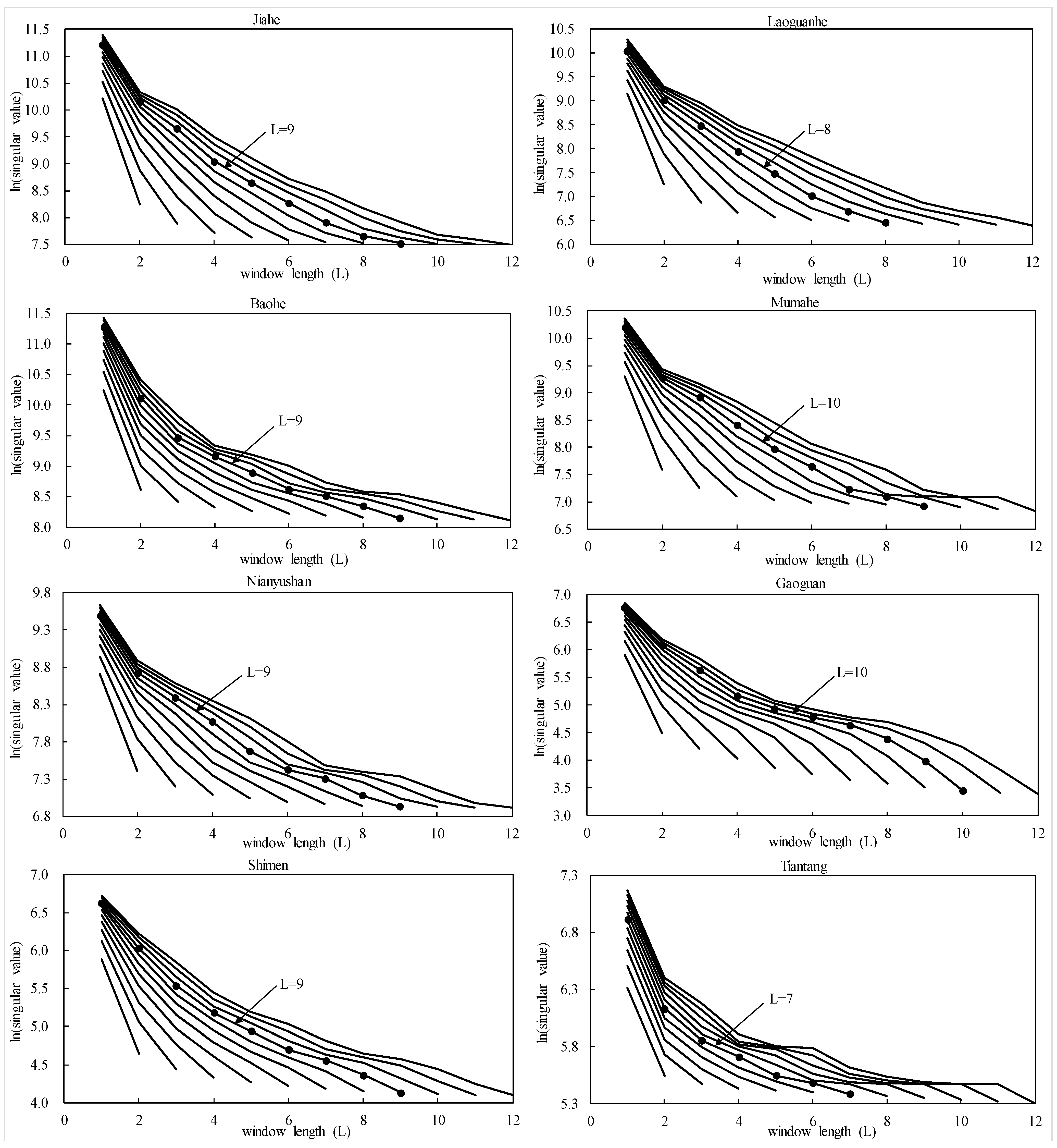
According to the theory of the SSA, the decomposition procedure requires identifying the parameter L. The value of an appropriate L should be able to clearly resolve different oscillations hidden in the original signal. In the current study, a small interval of [2,12] is examined to choose L [28]. L is considered as the target only if the singular spectrum can be markedly distinguished [33]. Figure 4 and Figure 5 present the relation between singular values and singular numbers for the rainfall and runoff series, respectively, where the singular values associated with the appropriate L are highlighted by the dotted solid line. It can be seen that L is selected as 8, 8, 8, 8, 9, 10, 9, and 7 for the rainfall series, and L is set as 9, 8, 9, 10, 9, 10, 9, and 7 for the runoff series in the Jiahe, Laoguanhe, Baohe, Mumahe, Nianyushan, Gaoguan, Shimen, and Tiantang watersheds, respectively.
Figure 4. Singular values as a function of different window length L for rainfall series.
Water 07 04144 g004
Once the original series is decomposed into L components, the subsequent task is to identify noise, choose the contributing components and reconstruct a new series as model inputs. This paper applied the cross-correlation function (CCF) to find the number of contributing components p (≤L). From the perspective of linear correlation, the positive or negative CCF value indicates that the component makes a positive or negative contribution to the output of model. Table 2 listed all CCF values between each decomposed component and original series for all watersheds. Take Jiahe rainfall series as an example; the last four components have positive CCF values, which mean that they have positive correlation with the original series. So the number of contributing components p is equal to 4 and the sum of the last four components is reconstructed series. Meanwhile, the reconstructed series of other time series can be obtained by the same way.
Figure 5. Singular values as a function of different window length L for runoff series.
Water 07 04144 g005
Table 2. Cross-correlation function (CCF) values between each decomposed component and original series.
WatershedDecomposed ComponentsLp
12345678910
Jiaherainfall−0.26−0.27−0.19−0.050.130.360.500.5584
runoff−0.14−0.15−0.11−0.050.050.180.390.550.7795
Laoguanherainfall−0.36−0.33−0.24−0.060.120.330.470.5384
runoff−0.15−0.15−0.100.000.140.350.550.7784
Baoherainfall−0.26−0.26−0.18−0.040.140.350.500.6084
runoff−0.18−0.20−0.16−0.080.040.160.330.540.7695
Mumaherainfall−0.34−0.32−0.22−0.060.130.340.470.5284
runoff−0.15−0.18−0.14−0.09−0.010.110.250.410.560.71105
Nianyushanrainfall−0.33−0.33−0.26−0.130.020.190.350.470.5195
runoff−0.22−0.22−0.16−0.030.150.340.540.6884
Gaoguanrainfall−0.32−0.37−0.30−0.18−0.070.090.230.370.460.43105
runoff−0.14−0.19−0.17−0.12−0.030.090.230.420.580.67105
Shimenrainfall−0.34−0.34−0.32−0.280.010.190.350.470.4895
runoff−0.21−0.23−0.18−0.090.040.190.390.580.6695
Tiantangrainfall−0.32−0.34−0.190.030.280.460.5374
runoff−0.31−0.31−0.160.030.250.460.6274

4. Results Analysis

Table 3 summarized the model performances for each watershed during calibration and testing periods. The ANN model is the benchmark in which the input is the original rainfall series without data preprocessing. It is shown that the model performance is improved significantly by data preprocessing techniques. During the testing period, the mean values of R2 and WB of eight watersheds are 70.16% and 0.879 by ANN, and are increased to 75.86% and 1.155 by NLPM-ANN, and 80.62% and 1.04 by SSA-ANN1, respectively. In the Tiantang watershed, the performance of the NLPM-ANN and SSA-ANN1 models is improved significantly, so the R2 value increased from 59.79% to 81.96% and 79.54%, respectively, during the testing period.
Table 3. Summary of model performances during calibration and testing periods.
WatershedANNNLPM-ANNSSA-ANN1SSA-ANN2
R2 (%)WBR2 (%)WBR2 (%)WBR2 (%)WB
Jiahecalibration68.191.02385.461.015`80.970.98296.091.013
testing61.480.86661.311.11974.910.97592.401.013
Laoguanhecalibration69.721.04885.661.04282.290.97296.311.186
testing60.421.05868.251.41278.441.46493.201.407
Baohecalibration64.750.97570.931.03988.501.02994.011.006
testing68.620.66769.380.89374.030.92794.310.956
Mumahecalibration80.640.95090.181.05087.860.97695.081.019
testing80.170.91385.61.41092.411.10894.711.053
Nianyushancalibration75.80.94183.441.08484.890.91085.861.020
testing82.380.80385.391.32988.300.93988.391.077
Gaoguancalibration66.161.03577.61.04580.171.00293.241.005
testing76.380.95777.970.89480.430.84089.850.962
Shimencalibration65.030.84864.851.06873.851.14194.531.084
testing720.77275.721.28176.901.08987.991.055
Tiantangcalibration65.470.98573.061.04978.080.96088.661.131
testing59.790.89581.960.95679.541.01591.321.043
Meancalibration69.470.97678.411.04682.081.0092.971.06
testing70.160.87975.861.15580.621.0491.521.07
The mean values of R2 and WB for the SSA-ANN1 model are 82.08% and 80.62%, and 1.0 and 1.04, during calibration and testing periods, respectively, which are much better than that of the NLPM-ANN model. It means that the reconstructed series obtained by SSA has a strong regularity and is easy to simulate. It also demonstrated that the impact of noise in hydrological time series on model performance is bigger than the seasonal hydrological behavior. Therefore, SSA is an effective way to improve runoff forecasting accuracy. The mean values of R2 for the SSA-ANN2 model are 92.97% and 91.52%, which are much better than those of the SSA-ANN1 model. It is concluded that considering previous runoff as a model input can improve model efficiency greatly.
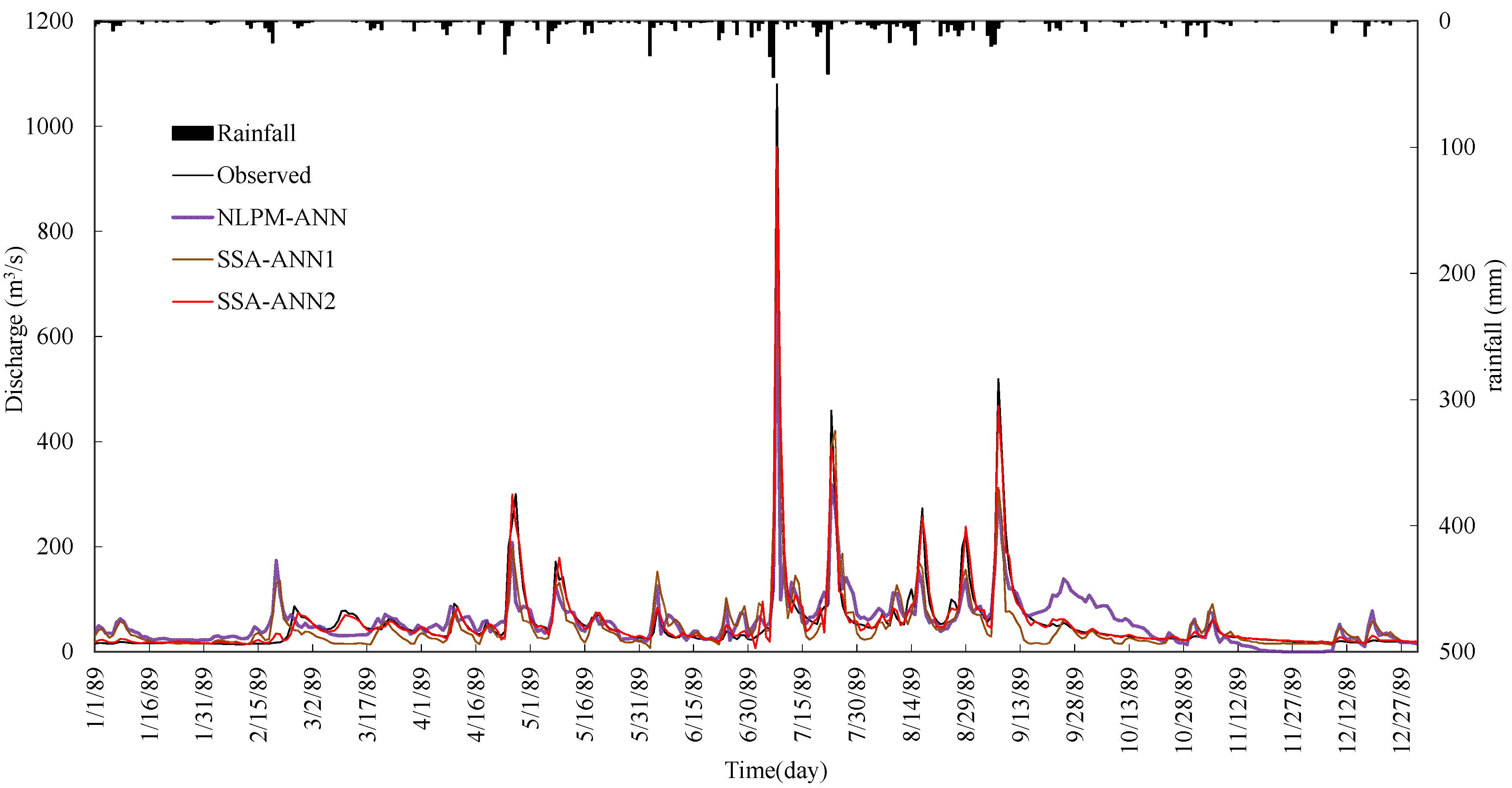
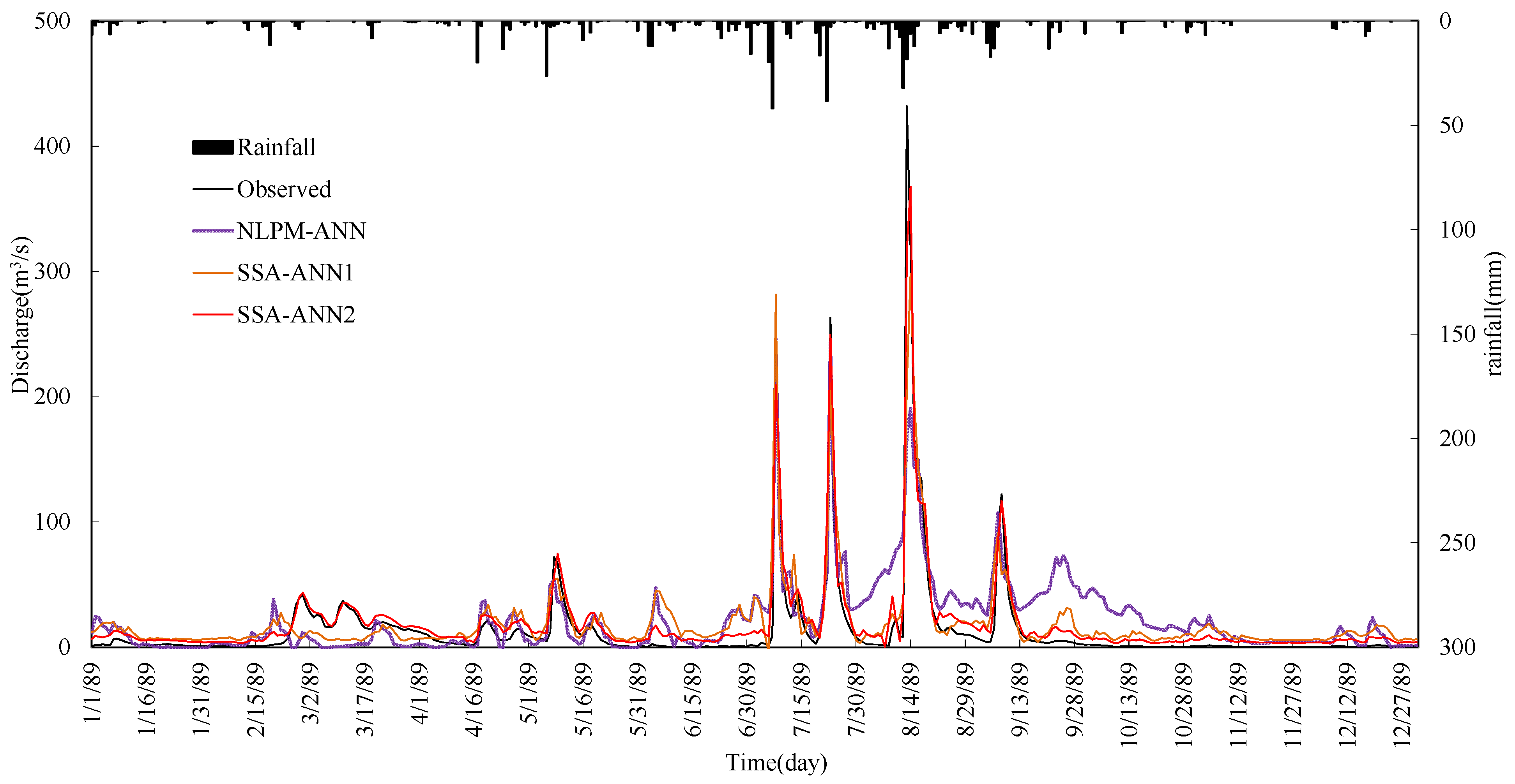
Figure 6. Observed and simulated runoff hydrographs by three models for Jiahe.
Water 07 04144 g006
Figure 7. Observed and simulated runoff hydrographs by three models for Laoguanhe.
Water 07 04144 g007
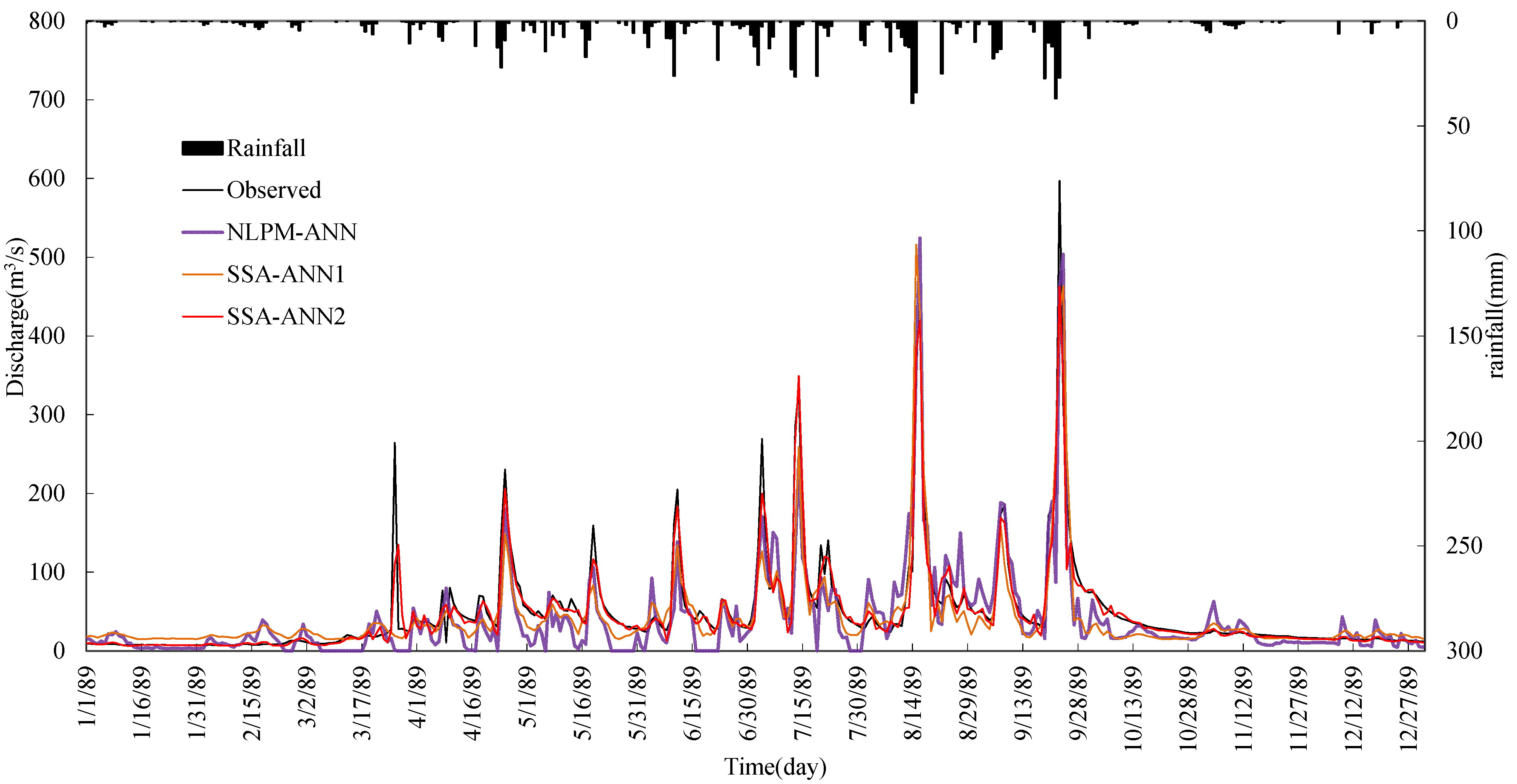
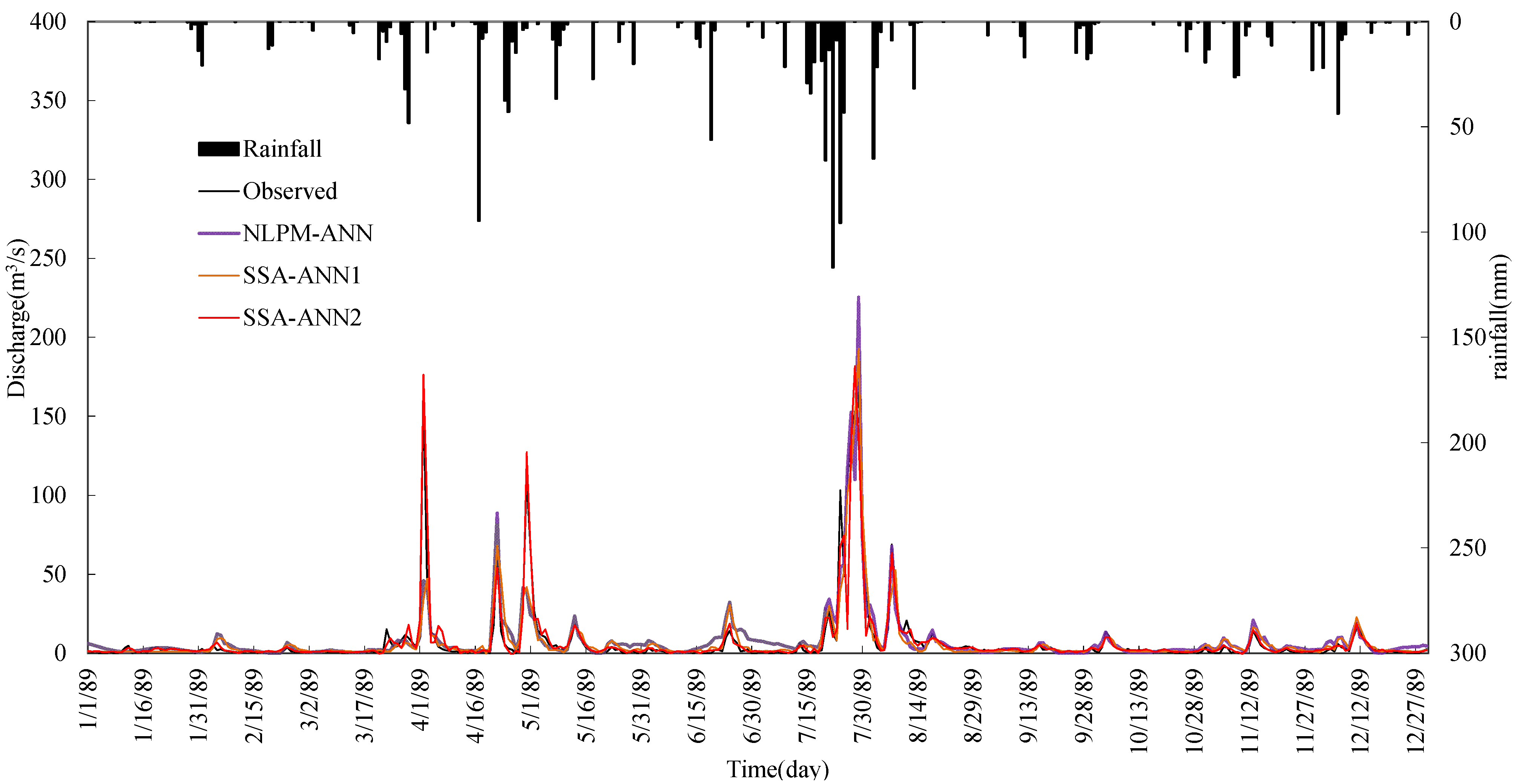
In order to compare the NLPM-ANN model, SSA-ANN1 model, and SSA-ANN2 model clearly and deeply, we selected one year during the testing period of four watersheds as an example, and the observed and simulated runoff hydrographs created by these three models for the Jiahe, Laoguanhe, Baohe, and Shimen watersheds are plotted in Figure 6, Figure 7, Figure 8 and Figure 9, respectively. These figures show that the runoff hydrograph simulated by the SSA-ANN2 model is much closer to the observational one. The peak and minimum flows simulated by the SSA-ANN2 model are the best among these models. Therefore, the SSA-ANN2 model can predict daily runoff very well in practice.
Figure 8. Observed and simulated runoff hydrographs by three models for Baohe.
Water 07 04144 g008
Figure 9. Observed and simulated runoff hydrographs by three models for Shimen.
Water 07 04144 g009

5. Summary and Conclusions

The objective of this study is to investigate the approach of improving daily runoff forecasting in terms of data preprocessing and model input selection. The black-box model ANN is selected as the benchmark. Considering the subtraction of the seasonal means from the original series can remove the nonlinearity of the rainfall-runoff process, the NLPM method was used to preprocess model inputs. Considering the hydrological time series can be viewed as a combination of quasi-periodic signals contaminated by noises, the SSA method was used to filter the noise and choose reconstructed series as model inputs. These two data preprocessing techniques were compared and analyzed. Main findings and discussions were summarized as follows:
(1)
The performance of the ANN model can be improved by data preprocessing techniques. SSA is more effective and it can improve the learning and training ability of the ANN type model significantly. Results also show that the impact of noise in hydrological time series on model performance is bigger than the seasonal hydrological behavior.
(2)
Comparing the SSA-ANN1 model with the NLPM-ANN model, the mean values of R2 and WB for the SSA-ANN1 model are 82.08% and 80.62%, and 1.0 and 1.04, during calibration and testing periods, respectively, which are much better than that of the NLPM-ANN model.
(3)
The SSA-ANN2 model performs best for daily runoff forecasting for all selected watersheds. The effective way for increasing daily runoff forecasting accuracy is to preprocess data series by SSA and select both previous related rainfall and runoff as predictive factors.
(4)
There are some limitations in this study. The method to select the contributing components relies on liner correlation analysis, which disregards the existence of nonlinearity in the hydrologic process. The sensitivities and uncertainties of model parameters are not analyzed. All of these will be the focus in our future research.

Acknowledgment

This study is financially supported by the National Natural Science Foundation of China (NSFC 51190094 and 51379148). The authors would like to thank the editor and anonymous reviewers whose comments and suggestions help to improve the manuscript.

Author Contributions

The SSA-ANN model was proposed and used to simulate the rainfall-runoff relationship. Results show that this model can improve daily runoff forecasting accuracy and it is worth of applying in practice.

Conflicts of Interest

The authors declare no conflict of interest.

References

  1. Baratti, R.; Cannas, B.; Fanni, A.; Pintus, M.; Sechi, G.M.; Toreno, N. River flow forecast for reservoir management through neural networks. Neurocomputing 2003, 55, 421–437. [Google Scholar] [CrossRef]
  2. Chang, F.J.; Chen, Y.C. A counterpropagation fuzzy-neural network modeling approach to real time streamflow prediction. J. Hydrol. 2001, 245, 153–164. [Google Scholar] [CrossRef]
  3. Nayak, P.C.; Sudheer, K.P.; Ramasastri, K.S. Fuzzy computing based rainfall–runoff model for real time flood forecasting. Hydrol. Process. 2005, 19, 955–968. [Google Scholar] [CrossRef]
  4. French, M.N.; Krajewski, W.F.; Cuykendall, R.R. Rainfall forecasting in space and time using a neural network. J. Hydrol. 1992, 137, 1–31. [Google Scholar] [CrossRef]
  5. Hsu, K.L.; Gupta, H.V.; Sorooshian, S. Artificial neural network modeling of the rainfall–runoff process. Water Resour. Res. 1995, 31, 2517–2530. [Google Scholar] [CrossRef]
  6. Sivakumar, B.; Liong, S.Y.; Liaw, C.Y. Evidence of chaotic behavior in Singapore rainfall. J. Am. Water Resour. Assoc. 1998, 34, 301–310. [Google Scholar] [CrossRef]
  7. Whigam, P.A.; Crapper, P.F. Modelling rainfall–runoff relationships using genetic programming. Math. Comput. Model. 2001, 33, 707–721. [Google Scholar] [CrossRef]
  8. Liong, S.Y.; Sivapragasm, C. Hood stage forecasting with SVM. J. Am. Water Resour. Assoc. 2002, 38, 173–186. [Google Scholar] [CrossRef]
  9. Govindaraju, R.S. Artificial neural networks in hydrology. I: Preliminary concepts. J. Hydrol. Eng. 2000, 5, 115–123. [Google Scholar]
  10. Govindaraju, R.S. Artificial neural networks in hydrology. II: Hydrological applications. J. Hydrol. Eng. 2000, 5, 124–137. [Google Scholar]
  11. Maier, H.R.; Dandy, G.C. Neural networks for the prediction and forecasting of water resources variables: A review of modelling issues and applications. Environ. Modell. Softw. 2000, 15, 101–124. [Google Scholar] [CrossRef]
  12. Dawson, C.W.; Wilby, R.L. Hydrological modeling using artificial neural networks. Progr. Phys. Geogr. 2001, 25, 80–108. [Google Scholar] [CrossRef]
  13. Sudheer, K.P.; Gosain, A.K.; Ramasastri, K.S. A data-driven algorithm for constructing artificial neural network rainfall-runoff models. Hydrol. Process. 2002, 16, 1325–1330. [Google Scholar] [CrossRef]
  14. Xiong, L.H.; O’Connor, K.M.; Guo, S.L. Comparison of three updating schemes using Artificial Neural Network in flow forecasting. Hydrol. Earth Syst. Sci. 2004, 8, 247–255. [Google Scholar] [CrossRef]
  15. Kumar, A.R.S.; Sudheer, K.P.; Jain, S.K.; Agarwal, P.K. Rainfall-runoff modelling using artificial neural networks: Comparison of network types. Hydrol. Process. 2005, 19, 1277–1291. [Google Scholar] [CrossRef]
  16. Pang, B.; Guo, S.L.; Xiong, L.H.; Li, C.Q. A nonlinear perturbation model based on artificial neural network. J. Hydrol. 2007, 333, 504–516. [Google Scholar] [CrossRef]
  17. Rezaeian, Z.M.; Amin, S.; Khalili, D.; Singh, V.P. Daily outflow prediction by multilayer perceptron with logistic sigmoid and tangent sigmoid activation functions. Water Resour. Manag. 2010, 24, 2673–2688. [Google Scholar] [CrossRef]
  18. Rezaeian, Z.M.; Stein, A.; Tabari, H.; Abghari, H.; Jalalkamali, N.; Hosseinipour, E.Z.; Singh, V.P. Assessment of a conceptual hydrological model and artificial neural networks for daily out-flows forecasting. Int. J. Environ. Sci. Technol. 2013, 10, 1181–1192. [Google Scholar] [CrossRef]
  19. Shamseldin, A.Y. Artificial neural network model for river flow forecasting in a developing country. J. Hydroinform. 2010, 12, 22–35. [Google Scholar] [CrossRef]
  20. Wu, J.S.; Han, J.; Annambhotla, S.; Bryant, S. Artificial neural networks for forecasting watershed runoff and stream flows. J. Hydrol. Eng. 2005, 10, 216–222. [Google Scholar] [CrossRef]
  21. Taormina, R.; Chau, K. Neural network river forecasting with multi-objective fully informed particle swarm optimization. J. Hydroinform. 2015, 17, 99–113. [Google Scholar] [CrossRef]
  22. Wu, C.L.; Chau, K.W.; Li, Y.S. Methods to improve neural network performance in daily flows prediction. J. Hydrol. 2009, 372, 80–93. [Google Scholar] [CrossRef]
  23. Nash, J.E.; Brasi, B.I. A hybrid model for flow forecasting on large catchments. J. Hydrol. 1983, 65, 125–137. [Google Scholar] [CrossRef]
  24. Liang, G.C.; Nash, J.E. Linear models for river flow routing on large catchments. J. Hydrol. 1988, 103, 157–188. [Google Scholar] [CrossRef]
  25. Sivapragasam, C.; Liong, S.Y.; Pasha, M.F.K. Rainfall and runoff forecasting with SSA-SVM approach. J. Hydroinform. 2001, 3, 141–152. [Google Scholar]
  26. Marques, C.A.F.; Ferreira, J.; Rocha, A.; Castanheira, J.; Goncalves, P.; Vaz, N.; Dias, J.M. Singular spectral analysis and forecasting of hydrological time series. Phys. Chem. Earth. 2006, 31, 1172–1179. [Google Scholar] [CrossRef]
  27. Wang, W.S.; Jin, J.L.; Li, Y.Q. Prediction of inflow at Three Gorges Dam in Yangtze River with wavelet network model. Water Resour. Manage. 2009, 23, 2791–2803. [Google Scholar] [CrossRef]
  28. Wang, Y.; Guo, S.L.; Chen, H.; Zhou, Y.L. Comparative study of monthly inflow prediction methods for the Three Gorges Reservoir. Stoch. Environ. Res. Risk Assess. 2014, 28, 555–570. [Google Scholar] [CrossRef]
  29. Wu, C.L.; Chau, K.W. Rainfall-runoff modeling using artificial neural network coupled with singular spectrum analysis. J. Hydrol. 2011, 399, 394–409. [Google Scholar] [CrossRef]
  30. Vautard, R.; Yiou, P.; Ghil, M. Singular-spectrum analysis: A toolkit for short, noisy and chaotic signals. Physica. D. 1992, 58, 95–126. [Google Scholar] [CrossRef]
  31. Golyandina, N.; Nekrutkin, V.; Zhigljavsky, A. Analysis of time Series Structure: SSA and the Related Techniques; CRC Press: Boca Raton, FL, USA, 2001. [Google Scholar]
  32. Toth, E.; Brath, A.; Montanari, A. Comparison of short-term rainfall prediction models for real-time flood forecasting. J. Hydrol. 2000, 239, 132–147. [Google Scholar] [CrossRef]
  33. Wu, C.L.; Chau, K.W.; Li, Y.S. Predicting monthly streamflow using data-driven models coupled with data-preprocessing techniques. Water Resour. Res. 2009, 45, 2263–2289. [Google Scholar] [CrossRef]