Spatiotemporal Correlations between Water Footprint and Agricultural Inputs: A Case Study of Maize Production in Northeast China

Abstract

To effectively manage water resources in agricultural production, it is necessary to understand the spatiotemporal variation of the water footprint (WF) and the influences of agricultural inputs. Employing spatial autocorrelation analysis and a geographically weighted regression (GWR) model, we explored the spatial variations of the WF and their relationships with agricultural inputs from 1998 to 2012 in Northeast China. The results indicated that: (1) the spatial distribution of WFs for the 36 major maize production prefectures was heterogeneous in Northeast China; (2) a cluster of high WFs was found in southeast Liaoning Province, while a cluster of low WFs was found in central Jilin Province, and (3) spatial and temporal differentiation in the correlations between the WF of maize production and agricultural inputs existed according to the GWR model. These correlations increased over time. Our results suggested that localized strategies for reducing the WF should be formulated based on specific relationships between the WF and agricultural inputs.

1. Introduction

Freshwater has an uneven temporal and spatial distribution from the perspective of availability and quantity. A growing population and increased demand for agricultural products have led to increasing competition for freshwater resources over the past several decades [1,2,3]. As a sector of intense water usage, agriculture is the largest user of freshwater, accounting for roughly 70% of total water usage [4,5,6]. Water scarcity is a major constraint in some agricultural production activities. Water usage for producing crops is expected to increase by 0.7% per year from its estimated level of 6400 billion m³·year⁻¹ in 2000 to 9060 billion m³·year⁻¹ by 2050 as a result of the need to feed a projected global population of 9.2 billion [7,8]. As a result, it is important to evaluate water resource utilization in agricultural production to meet future freshwater supply challenges [9,10].

The water footprint (WF) concept provides a new way of evaluating water utilization in agricultural production [11]. For a given crop, the WF refers to the total amount of freshwater that is consumed and contaminated in the crop production process. It contains three components: the amount of rainwater consumed, the amount of irrigation water in the form of surface or ground water consumed, and the amount of freshwater required to assimilate the load of pollutants [12]. These components are defined as green WF, blue WF and grey WF, respectively [13,14]. The WF has led to a better understanding of the water requirement of crop production, which is attracting increased attention and has motivated a large number of studies [15,16,17,18,19]. Thus far, several studies have shed light on the spatial differences in the WFs of a variety of types of crops production in China. Sun et al. assessed the spatiotemporal variability of the WF for grain in an irrigation district of China during 1960–2008 [20]. Tian et al. analysed the temporal and spatial variation of the WF of China’s five major food crops from 1978 to 2010 [21]. Wang et al. calculated and compared the WF of each grain crop and the integrated WFs of grain products with actual and virtual crop patterns in various regions of China for 2010 [22]. These previous studies suggested that the WF exhibits variability in different regions at the national level. However, to the best of our knowledge, few studies have tried to explore the spatial pattern characteristics of the WF at the prefecture level. Studies regarding the WF prefecture levels are more important because they can directly relate water usage to crop production. Besides, the underlying factors influencing WFs were mostly investigated from the perspective of climate. In fact, the WF of crop production primarily depends on agricultural inputs rather than the regional climate and its variation [23]. Therefore, it is essential to investigate the relationships between the WF and agricultural inputs.

To better understand the correlations between the WF of crop production and agricultural inputs, an integrated approach is much needed. The geographically weighted regression (GWR) model is an expansion of the classical multivariate linear regression model, which considers not only the spatial non-stationary of relationships but also, in part, the spatial dependence, as it relies on local rather than global parameters [24]. Additionally, the GWR model has been applied in social economics, urban geography, meteorology, forestry and many other disciplines [25,26,27]. Few studies have been conducted on the analysis of correlations between the WF and agricultural inputs over space with the GWR method.

We selected Northeast China, which provides one-third of China’s food production, as our study region. In this region, maize is one of the primary crops. The major objectives of this paper were: (1) to determine the spatial distribution of the WF of maize production at the prefecture level; (2) to identify the spatial patterns and clusters of the WF using global and local spatial autocorrelation analyses; and (3) to analyse the spatial relationship between the WF and the three agricultural inputs based on the GWR model. This study could provide valuable information for designing and implementing effective measures for reducing the WF of maize production in Northeast China.

2. Material and Methods

2.1. Study Area

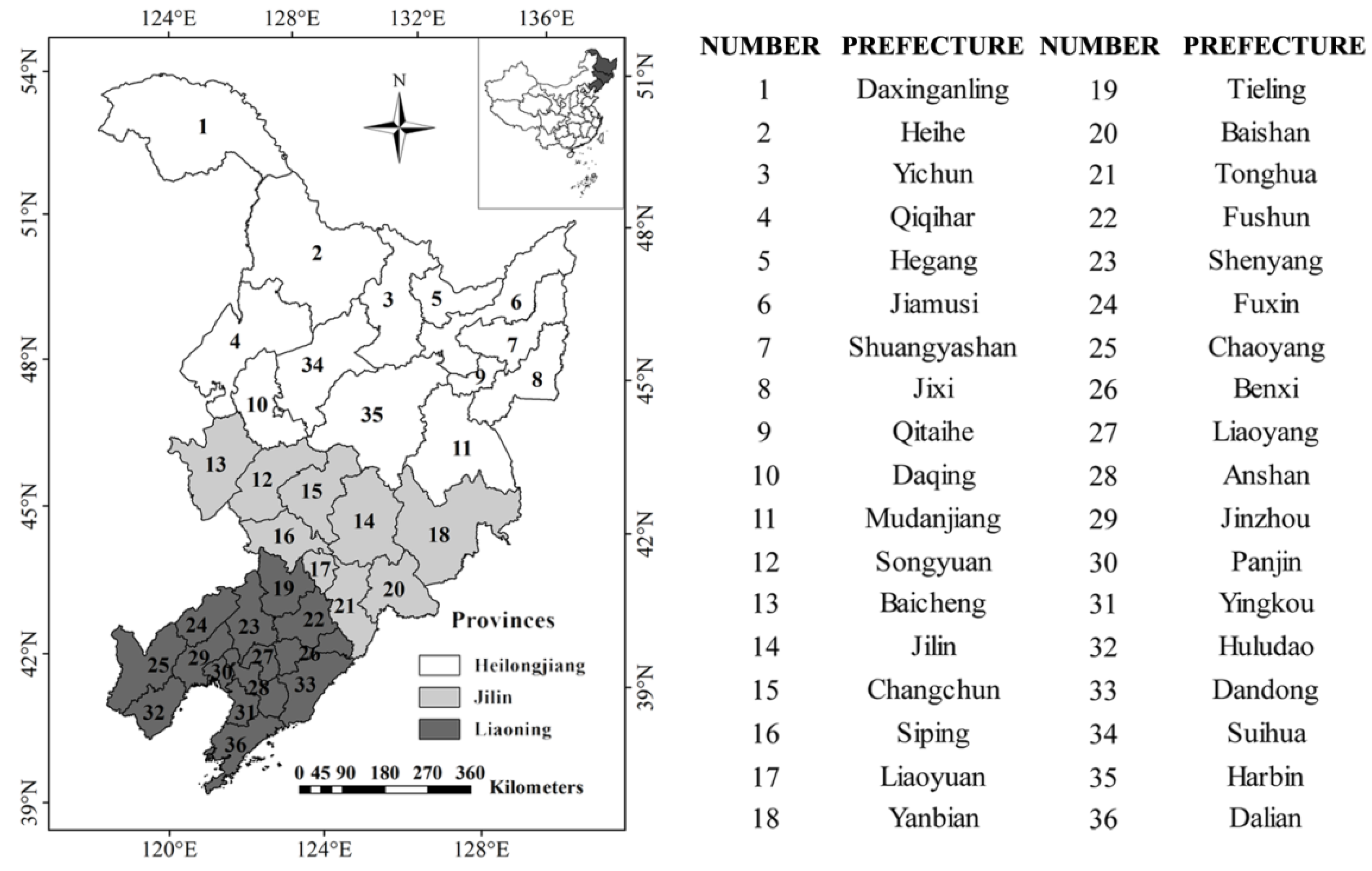
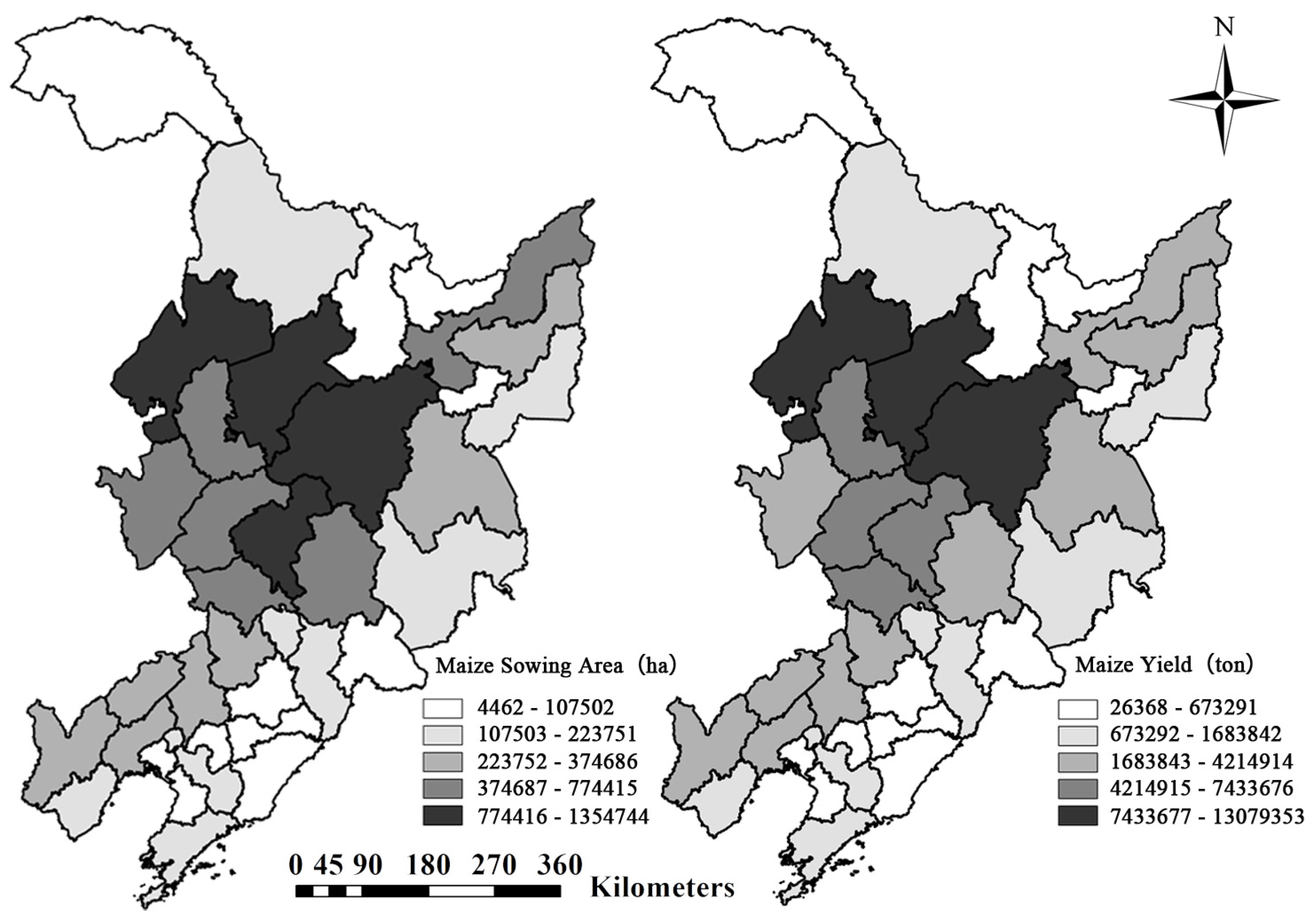
Northeast China is located between 118°53′–135°05′ E and 38°43′–53°33′ N, and consists of Liaoning, Jilin, and Heilongjiang Provinces (Figure 1). The region covers an area of 7.92 × 10⁵ km², of which farmland occupies 2.64 × 10⁵ ha, representing 16.5% of the total arable land in China [28]. The maize sowing area and yield at the prefecture level in 2012 are shown in Figure 2. The climate in the region is cold temperate and humid in the north and semi-humid in the west. The mean annual air temperature ranged from −4.2 °C to 10.9 °C, decreasing from south to north. The precipitation is generally concentrated in the summer and autumn (from May to October) [29], which coincides with the growing period of maize in Northeast China. The annual precipitation decreased from the southeast (1070 mm) to the northwest (450 mm). Maize, as the major grain crop in Northeast China, is highly seasonal with a single crop each year. The differences in the physical geography significantly affect the growth periods and crop coefficients of maize in each province [30] (Table 1).

Figure 1. Location of Northeast China and the names of its 36 prefectures in three provinces.

Figure 1. Location of Northeast China and the names of its 36 prefectures in three provinces.

Figure 2. The maize sowing area and yield at the prefecture level in 2012.

Figure 2. The maize sowing area and yield at the prefecture level in 2012.

Table 1. Growth periods and literature values of crop coefficient K_c for maize in Liaoning, Jilin and Heilongjiang Provinces.

Province	Growth Periods			Crop Coefficients (Kc)
	Sowing Date	Harvesting Date	Total Days	Initial Season (Kc ini)	Mid-Season (Kc mid)	Late-Season (Kc late)
Liaoning	25-April	20-September	149	0.38	1.22	0.60
Jilin	1-May	24-September	147	0.40	1.22	0.58
Heilongjiang	16-May	30-September	137	0.36	1.20	0.55

Note: Source: China Meteorological Data Sharing Service System and Huang et al. (2011) [30].

Table 1. Growth periods and literature values of crop coefficient K_c for maize in Liaoning, Jilin and Heilongjiang Provinces.

Province	Growth Periods			Crop Coefficients (Kc)
	Sowing Date	Harvesting Date	Total Days	Initial Season (Kc ini)	Mid-Season (Kc mid)	Late-Season (Kc late)
Liaoning	25-April	20-September	149	0.38	1.22	0.60
Jilin	1-May	24-September	147	0.40	1.22	0.58
Heilongjiang	16-May	30-September	137	0.36	1.20	0.55

Note: Source: China Meteorological Data Sharing Service System and Huang et al. (2011) [30].

2.2. Data Sources

The climate data of 36 weather stations, one location per prefecture, were taken from the China Meteorological Data Sharing Service System [31] for the period of 1998 to 2012, including monthly average maximum and minimum temperature, relative humidity, wind speed, sunshine hours and precipitation. The agricultural data, including maize yield, maize sowing area, agricultural machinery power, effective irrigation area and consumption of chemical fertilizers, were obtained from the statistical yearbooks 1998–2012 of the three provinces.

2.3. Methods

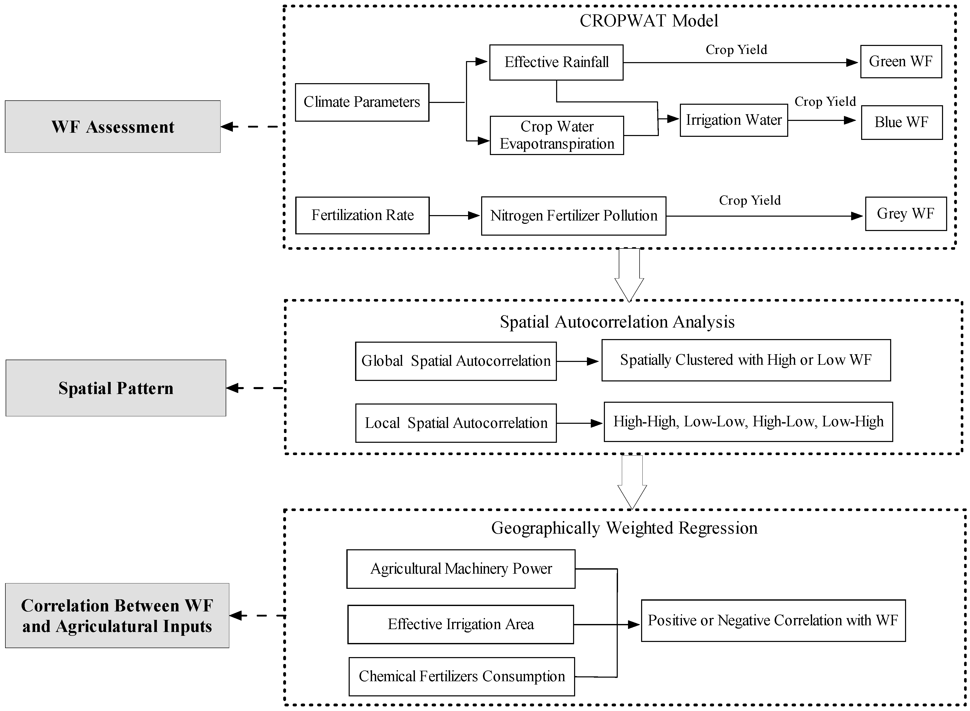
First, the WFs of maize production were accounted for in Northeast China. Next, the spatial patterns of the WF were investigated. Finally, the relationships between the WF and agricultural inputs were explored. The overall calculation process flow chart is diagrammed in Figure 3.

Figure 3. Diagram for WF assessment and the correlations between WF and agricultural inputs.

Figure 3. Diagram for WF assessment and the correlations between WF and agricultural inputs.

2.3.1. WF Calculation Methodology

The WF of crop production was estimated following the calculation framework developed by Hoekstra et al. [14], which is the total water consumption during crop growth process, including blue WF, green WF and grey WF [32], namely:

$$W{F}_{\text{total}}=W{F}_{\text{green}}+W{F}_{\text{blue}}+W{F}_{\text{grey}}$$

(1)

where WF_total is the WF of crop production(m³·ton⁻¹); WF_green is the green WF (m³·ton⁻¹); WF_blue is the blue WF (m³·ton⁻¹); and WF_grey is the grey WF (m³·ton⁻¹).

The WF_green and WF_blue are calculated as crop water use divided by crop yield. The green and blue water use is calculated by accumulation of daily evapotranspiration over the growing period.

$$W{F}_{\text{green}}=\frac{CW{U}_{\text{green}}}{Y}=10\times \frac{E{T}_{\text{green}}}{Y}$$

(2)

$$W{F}_{\text{blue}}=\frac{CW{U}_{\text{blue}}}{Y}=10\times \frac{E{T}_{\text{blue}}}{Y}$$

(3)

where CWU_green and CWU_blue are green and blue water usage (mm); ET_green and ET_blue are green and blue water evapotranspiration (mm); Y is the crop yield (ton·ha⁻¹); and the factor 10 converts water depths in millimetres into water volumes per land surface in m³·ha⁻¹.

The WF_grey is calculated as the chemical application rate to the field per hectare (AR, kg·ha⁻¹) times the leaching-run-off fraction (α) divided by the maximum acceptable concentration (C_max, kg·m⁻³) minus the natural concentration for the pollutant considered (C_nat, kg·m⁻³) and divided by the crop yield (Y, ton·ha⁻¹).

$$W{F}_{\text{grey}}=\frac{(\text{α}\times AR)/(C_{\max }-C_{\text{nat}})}{Y}$$

(4)

Considering the availability of local data, in this study, we quantified the grey WF related to nitrogen use only. We have further taken α as 10% following Chapagain et al. [12], C_nat as zero, and C_max as 12 mg·L⁻¹ following China water quality standards.

2.3.2. ET Calculations Based on the CROPWAT Model

The green and blue water evapotranspiration are estimated based on crop water requirement by employing the CROPWAT 8.0 model [33,34], which are calculated as:

$$E{T}_{\text{green}}=\min (E{T}_{\text{c}},P_{\text{eff}})$$

(5)

$$E{T}_{\text{blue}}=\max (0,E{T}_{\text{c}}-P_{\text{eff}})$$

(6)

where ET_c is the crop evapotranspiration and P_eff is the effective precipitation over the crop growing period (mm).

ET_c is calculated by employing the CROPWAT model based on the FAO Penman-Monteith method [35].

$$E{T}_{\text{c}}=K_{\text{c}}E{T}_0$$

(7)

where K_c is the crop coefficient; ET₀ is the reference evapotranspiration, calculated as follows:

$$E{T}_0=\frac{0.408\mathrm{\Delta }\left(R_{\text{n}}-G\right)+\text{γ}\frac{900}{T+273}{U}_2\left(e_{\text{s}}-e_{\text{a}}\right)}{\mathrm{\Delta }+\text{γ}\left(1+0.34U_2\right)}$$

(8)

where R_n is the net radiation (MJ·m⁻²·d⁻¹); G the soil heat flux (MJ·m⁻²·d⁻¹); T the average air temperature (°C); U₂ the wind speed at 2 m height (m·s⁻¹); e_s the saturation vapor pressure (kPa); e_a the actual vapor pressure (kPa); Δ the slope of saturation vapor pressure versus air temperature curve (kPa·°C⁻¹); the hygrometer constant (kPa·°C⁻¹).

P_eff is calculated according to a formula developed by the USDA Soil Conservation Service [34,36]:

$$P_{\text{eff}}=\{\begin{array}{c}P/125(125-0.2P)\\ 125+0.1P\end{array}\begin{array}{c}\\ \end{array}\begin{array}{c}P\le 250\\ P>250\end{array}$$

(9)

where P is the precipitation at a month step (mm).

2.3.3. Spatial Autocorrelation

Both global and local spatial autocorrelation test results are used to confirm the presence of strong spatial dependence and heterogeneity in the distribution of the WF, supporting the use of the GWR technique.

Global Moran’s I is applied to detect the overall degree of spatial autocorrelation among the regions. The equation is given as:

$$I\text{=}\frac{n{\displaystyle \sum _{i=1}^n{\displaystyle \sum _{j=1}^n{W}_{ij}(X_i-\overline{X})(X_j-\overline{X})}}}{({\displaystyle \sum _{i=1}^n{\displaystyle \sum _{j=1}^n{W}_{ij}}})\cdot {\displaystyle \sum _{i=1}^n{(X_i-\overline{X})}^2}}$$

(10)

where n is the number of spatial unit; X_i and X_j are the values of WF of spatial units i and j, respectively; $\overline{X}$ is the mean of X; W_ij is a matrix of spatial weight applied to the comparison between spatial units i and j. Generally, W is defined using an adjacency standard. When the units i are adjacent to units j, W_ij is equal to 1, otherwise W_ij is equal to 0. The value of Moran’s I varies between −1 and 1. The significance of the spatial autocorrelation can be tested by Z statistics, which is given as:

$$Z=\frac{1-E(I)}{\sqrt{Var(I)}}$$

(11)

where E(I) and Var(I) denote the expectation value and the variance of Moran’s I, respectively [37]. If Z-value is greater than 0 and statistically significant, an obvious positive autocorrelation exists in the spatial distribution [38].

The local indicator of spatial autocorrelation index (LISA) takes each spatial unit as the inspection object and analyses its properties of spatial autocorrelation [39]. The equation is given as:

$$I_i=Z_i{\displaystyle \sum W_{ij}}{Z}_j$$

(12)

where I_i is the local autocorrelation index of WFand Z_i and Z_j are the standardization of values of WF of spatial units i and j.

2.3.4. Geographically Weighted Regression (GWR) Model

The GWR model extends the traditional regression framework by embedding the spatial location of the data into the regression parameter [40,41]. The local estimation of the parameters with GWR is expressed as follows [42]:

$$\begin{array}{cc}{y}_i={\beta }_0(u_i,v_i)+{\displaystyle \sum _k{\text{β}}_k}(u_i,v_i)x_{ik}+{\text{ε}}_i& i=1,2,\mathrm{...},n\end{array}$$

(13)

where y_i is the dependent variable in the ith location; x_ik is the ith value of the kth independent variable; k represents the number of independent variables; i represents the number of samplings; (u_i, v_i) denotes the coordinates; β₀ (u_i, v_i) represents the intercept value, and β_k (u_i, v_i) is the continued function; ε_i represents the model residual.

To calculate the spatial distribution of the weightings, the optimal bandwidth is required. The Cross-Validation (CV) or Akaike Information Criterion (AIC) is usually used for calculation. In this paper the AIC was chosen, which was fixed by the maximum likelihood principle to determine the optimal bandwidth [43].

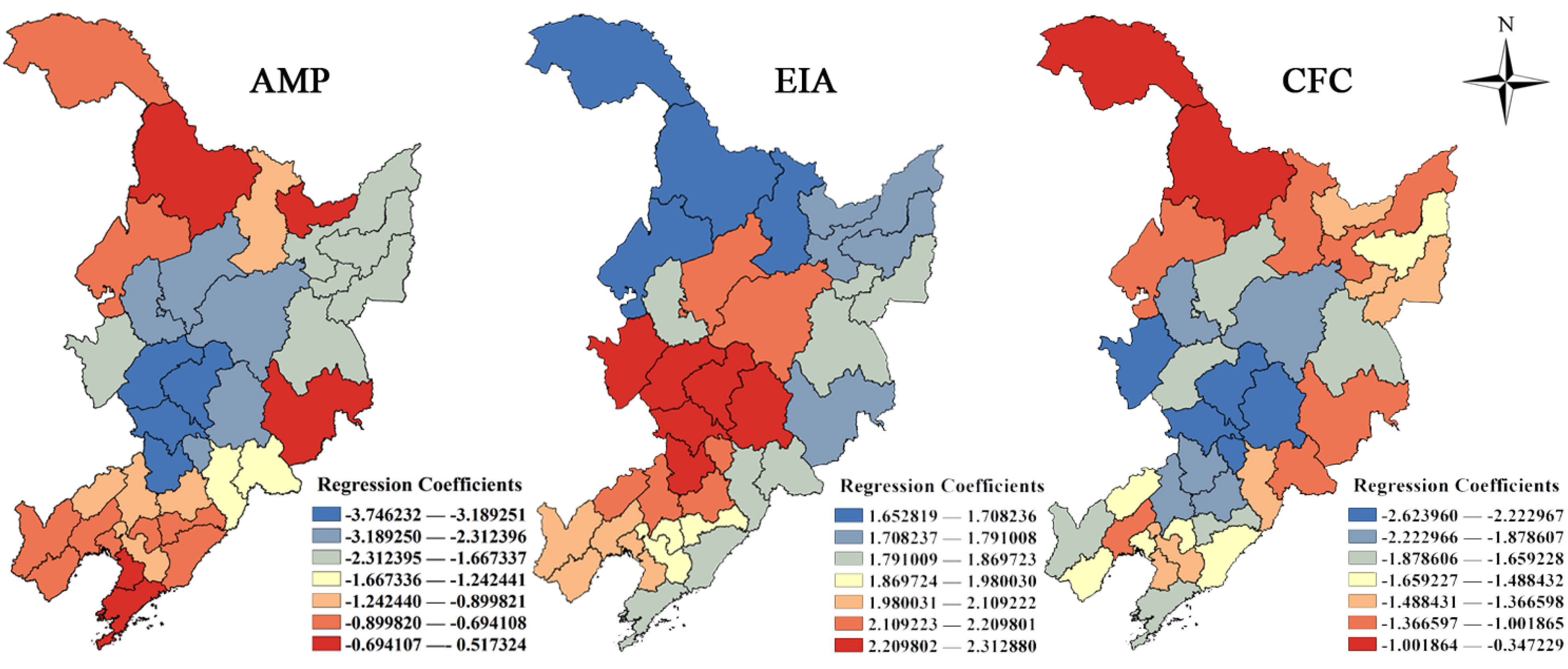
GWR model analysis was performed using the software ArcGIS10.1. In this study, the WF of maize production was treated as the dependent variable, and three agricultural inputs, namely, agricultural machinery power (AMP), effective irrigation area (EIA) and chemical fertilizers consumption (CFC) were chosen as the independent variables of the models.

3. Results

3.1. Spatial Distribution of WF of Maize Production

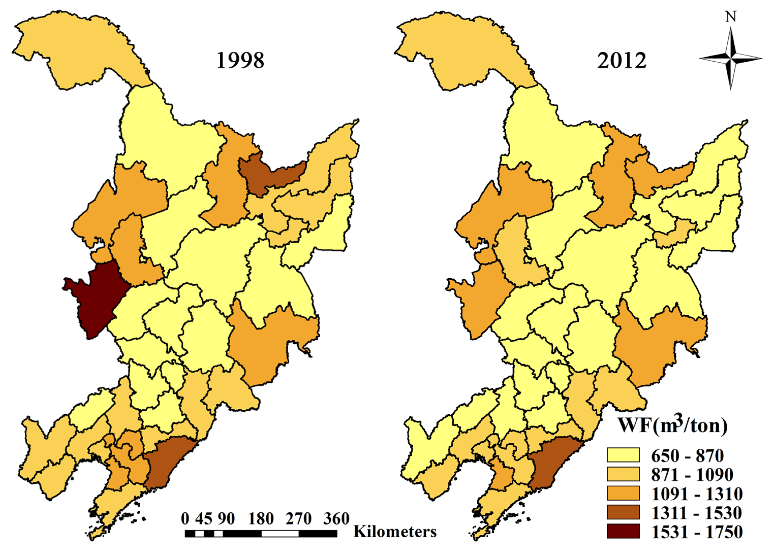
From 1998 to 2012, the average annual WF of maize production was 1029 m³·ton⁻¹ in Northeast China. Green WF was the biggest part of the total WF of maize production with the proportion at 51%, followed by grey and blue WF, which accounted for 28% and 21%, respectively. This suggests that the WF of maize production in this region largely relies on green water resources, i.e., consumptive use of rainwater, which had a non-uniform seasonal distribution.

The WF of maize production exhibited significant differences on the prefecture level. As can be seen from 1998, the highest values of WF were observed in Baicheng, where it was 1608 m³·ton⁻¹ (Figure 4). This could be explained by the highest evapotranspiration. Dandong took second place with 1347 m³·ton⁻¹. The lowest WFs were calculated for Siping with 691 m³·ton⁻¹, and Tieling with 756 m³·ton⁻¹, which could be explained by the higher maize yields in these two prefectures. Compared to 1998, the WFs of all prefectures showed a decreasing trend in 2012. Dandong had replaced Baicheng with the highest WF, which was 1313 m³·ton⁻¹, followed by Baicheng with 1291 m³·ton⁻¹. Tieling had replaced Siping as the prefecture with the lowest WF, which was 667 m³·ton⁻¹. Siping ranked second, with a value of 672 m³·ton⁻¹.

Figure 4. Spatial distribution of WF of maize production in 1998 and 2012.

Figure 4. Spatial distribution of WF of maize production in 1998 and 2012.

3.2. Spatial Pattern Characteristics of the WF of Maize Production

Both the global and local spatial autocorrelation test results confirm the presence of strong spatial dependence and heterogeneity in the distribution of the WF, supporting the use of the GWR technique.

Global Moran’s I of WFs in 1998 and 2012 (Table 2) were 0.5512 and 0.5530, respectively, and all Z-values were significant (p-value = 0.01, with 999 permutations), which demonstrated a positive spatial correlation of prefecture-level WFs in the entire study region. In other words, prefecture units with higher and lower levels of WFs were spatially clustered. Meanwhile, the spatial autocorrelation of WFs in 2012 was slightly stronger than that in 1998.

Table 2. Global Moran’s I of water footprints (WFs) of maize production in 1998 and 2012.

Year	Moran’s I	Z-Value	p-Value
1998	0.5512	2.6366	0.01
2012	0.5530	2.4741	0.01

Table 2. Global Moran’s I of water footprints (WFs) of maize production in 1998 and 2012.

Year	Moran’s I	Z-Value	p-Value
1998	0.5512	2.6366	0.01
2012	0.5530	2.4741	0.01

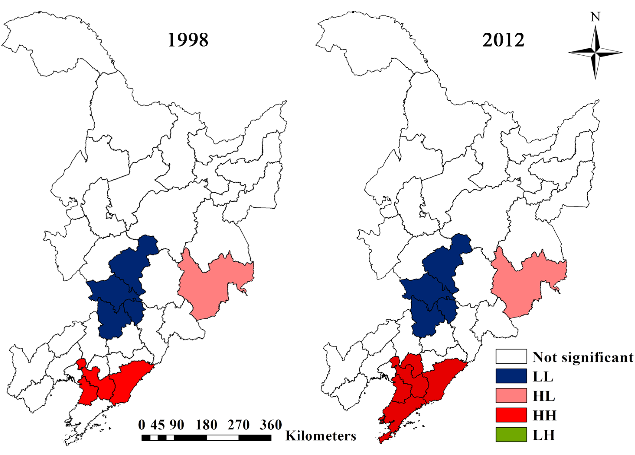
As for the local spatial autocorrelation, LISA statistics can be classified into four categories and mapped in a LISA cluster map (Figure 5). For instance, prefectures that have high WFs surrounded by high WFs (HH) and those with low WFs surrounded by low WFs (LL) represent potential spatial clusters. Prefectures with high WFs surrounded by low WFs (HL) and low WFs surrounded by high WFs (LH) suggest potential spatial outliers. The cluster of high WF values (HH) was located in southeast Liaoning in 1998 (composed of the three prefectures of Dandong, Anshan and Yingkou), but it increased in 2012 (composed of the five prefectures of Dandong, Liaoyang, Anshan, Yingkou and Dalian), indicating that the WF disparity in this region decreased. The cluster of low WF values (LL) included the four prefectures of Changchun, Siping, Liaoyuan and Tieling, which were primarily located in central Jilin Province, and the number of prefectures in this cluster remained relatively stable. Other forms of local spatial autocorrelation included one HL-type prefecture (Yanbian) in both years.

Figure 5. LISA cluster map for WFs of maize production in 1998 and 2012.

Figure 5. LISA cluster map for WFs of maize production in 1998 and 2012.

3.3. Spatial Variations in Correlations between Agricultural Inputs and the WF of Maize Production

Table 3 summarizes the results of the GWR between the WF and agricultural inputs. Results of the GWR models demonstrated that the R² and adjusted R² values in 1998 and 2012 were approximately equal, both representing over 63% of the total variance of the WF. The local parameters are described by six-number summaries consisting of the minimum, maximum, mean, lower quartile, median and upper quartile values, which presented large differences. In 1998, the correlation between the EIA and the WF was still positive; however, the AMP and CFC were either positive or negative. In 2012, the correlations between the AMP, EIA and the WF were positive and the CFC was negative.

Table 3. Statistical description of the geographically weighted regression (GWR) model parameter for 1998 and 2012.

Descriptive Index	1998			2012
	AMP	EIA	CFC	AMP	EIA	CFC
Minimum value	−2.283	0.464	−1.624	−3.746	1.653	−2.624
Maximum value	0.933	2.033	0.369	−0.517	2.313	−0.347
Mean	−0.591	1.315	−0.657	−1.550	1.977	−1.598
Upper quartile	−1.610	1.091	−1.113	−2.262	1.814	−1.902
Median	−0.350	1.373	−0.648	−1.039	1.961	−1.547
Lower quartile	0.460	1.539	−0.205	−0.748	2.174	−1.368
AIC	481.242			487.305
R2	0.635			0.631
Adjusted R2	0.581			0.593

Notes: AMP: Agricultural machinery power; EIA: Effective irrigation area; CFC: Chemical fertilizers consumption.

Table 3. Statistical description of the geographically weighted regression (GWR) model parameter for 1998 and 2012.

Descriptive Index	1998			2012
	AMP	EIA	CFC	AMP	EIA	CFC
Minimum value	−2.283	0.464	−1.624	−3.746	1.653	−2.624
Maximum value	0.933	2.033	0.369	−0.517	2.313	−0.347
Mean	−0.591	1.315	−0.657	−1.550	1.977	−1.598
Upper quartile	−1.610	1.091	−1.113	−2.262	1.814	−1.902
Median	−0.350	1.373	−0.648	−1.039	1.961	−1.547
Lower quartile	0.460	1.539	−0.205	−0.748	2.174	−1.368
AIC	481.242			487.305
R2	0.635			0.631
Adjusted R2	0.581			0.593

Notes: AMP: Agricultural machinery power; EIA: Effective irrigation area; CFC: Chemical fertilizers consumption.

The relationships between the WF and agricultural inputs were spatially non-stationary (Figure 6 and Figure 7). In 1998, most regression coefficients of the AMP were found to be negative, except for south-central Liaoning Province. The CFC had a positive correlation with the WF in most areas, other than south Liaoning Province. The EIA had a positive correlation with the WF in the entire region. Compared to 1998, the regression coefficients of all agricultural inputs increased in 2012, suggesting the correlations were becoming stronger. Overall the correlations of the AMP and CFC were changing from positive to negative. The AMP and CFC had negative correlation with the WF in the entire region, while the EIA still had a positive correlation with the WF. The absolute value of regression coefficient of the AMP, EIA and CFC all exhibited a decreasing trend from the centre to the south and north.

Figure 6. Spatial distribution of regression coefficients of agricultural inputs in 1998.

Figure 6. Spatial distribution of regression coefficients of agricultural inputs in 1998.

Figure 7. Spatial distribution of regression coefficients of agricultural inputs in 2012.

Figure 7. Spatial distribution of regression coefficients of agricultural inputs in 2012.

4. Discussion

In this study, we mapped the distribution of the WF of maize production at the prefecture level in Northeast China. A combination of the climatic condition, growing period and fertilizer consumption lead to the diversity of the WFs among 36 prefectures. The distribution of the WF in Northeast China was clustered, indicated by the significantly global Moran’s I values. The LISA method detected the regions with high or low concentrations of WF. The spatial clustered regions with high WF of maize production were distributed in southeast Liaoning Province. The soils in these regions are poor and essentially unsuitable for crop production. The spatial clustered regions with low WF of maize production were distributed in central Jilin Province, which is located on the Songnen Plain and considered the Golden-Maize-Belt in China. It can be attributed to such factors as favourable climate condition, soil quality, proper irrigation facilities and relatively higher maize yield. These findings can help policy-makers prioritize maize production area and optimize maize production distribution.

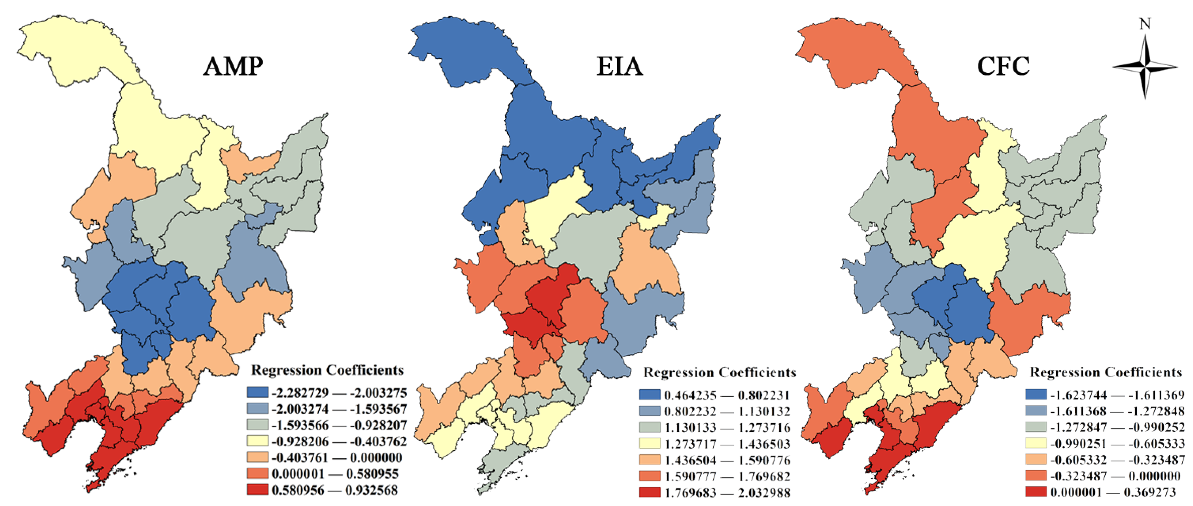
The factors impacting the WF are miscellaneous. To explore the WF and its influence mechanisms, scholars began to study the relationships between WF and individual factors, such as climatic factors and agricultural input [23,44,45]. The methodology employed in this study only included correlation analysis. However, in reality, the relationships between the WF and influential factors are not always consistent in different areas. In particular, we employed the GWR technique to examine the spatial and temporal differences in the correlation between three agricultural inputs and the WF of maize production, including the AMP, EIA and CFC. The regression coefficients of the GWR also displayed a high variability in space, which could better explain the spatial differences of the correlation between the agricultural inputs and the WF. The spatial variations in the relationships are affected by the level of agricultural development.

In addition, the GWR analysis can help decision-makers clearly see the results of past relationships between the WF and agricultural inputs on a local scale and make appropriate decisions for future planning to reduce the WF of maize production. According to the results of the GWR model, the correlation between the AMP and WF was mainly positive in the study area. Attention should be paid to improving the mechanical technologies. The AMP in south-central Liaoning shifted from a positive to a negative correlation with the WF, so the amount of machinery should be adjusted appropriately. The correlation between the EIA and WF was positive in the study area. Thus, irrigation water should be reduced in this region. Water-saving irrigation techniques, such as drip or sprinkler irrigation, should be employed appropriately to inhibit the growing WF. The CFC had a negative correlation with the WF, which indicated that properly managed fertilizer use contributed to reducing the WF. Meanwhile, the CFC shifted from a positive to a negative correlation with the WF in south Liaoning. In these areas, increasing fertilizer usage or adjusting the fertilizer proportions and increasing the usage of organic fertilizers should be considered.

To the best of our knowledge, this is the first study focusing on the spatial pattern of the WF and the relationships between the WF and agricultural inputs. Nevertheless, there are still limitations in this study. There are some uncertainties in the quantification of the WF of maize production. On the one hand, the agricultural data were primarily derived from statistical data, and there are discrepancies between these values and reality. On the other hand, the grey WF was estimated based on a simplified approach, which left out local factors that influence the precise leaching rates. In addition, our spatial analysis was based on the prefecture scale, but the distribution of the WF was also not homogeneous at the prefecture level. Therefore, this study cannot identify the spatial heterogeneity within each unit.

5. Conclusions

The spatial distribution and cluster areas of the WFs of maize production in Northeast China were investigated and the relationships between the WF and agricultural inputs were explored. The results demonstrated that the spatial differences of the WFs of maize production were obvious in Northeast China. Two cluster regions were detected. The prefectures with higher WFs were formed in southeast Liaoning Province while the prefectures with lower WFs were formed in central Jilin Province. From the perspective of the GWR results, the WF and agricultural inputs relationships were significantly spatially non-stationary. Finally, the combination of the GWR along with the GIS approaches constitutes a powerful tool for better displaying spatiotemporally varying relationships between the WF and agricultural inputs. Extension of this study could focus on adding other driving forces, such as population, plantation structure and policy in the spatiotemporal analysis of the WF in the studied areas.

References

- Falkenmark, M.; Rockstrom, J.; Karlberg, L. Present and future water requirements for feeding humanity. Food Secur. 2009, 1, 59–69. [Google Scholar] [CrossRef]
- De Fraiture, C.; Wichelns, D. Satisfying future water demands for agriculture. Agric Water Manag. 2010, 97, 502–511. [Google Scholar] [CrossRef]
- Ercin, A.E.; Hoekstra, A.Y. Water footprint scenarios for 2050: A global analysis. Environ. Int. 2014, 64, 71–82. [Google Scholar] [CrossRef] [PubMed]
- Molden, D.; Oweis, T.; Pasquale, S.; Kijne, J.; Hanjra, M.A.; Bindraban, P.; Bouman, B.; Cook, S.; Erenstein, O.; Farahani, H. Water for food, water for life, a comprehensive assessment of water management in agriculture. In Pathways for Increasing Agricultural Water Productivity; Earthscan and International Water Management Institute: London, UK; Colombo, Sri Lanka, 2007; pp. 279–310. [Google Scholar]
- Xiong, W.; Holman, I.; Lin, E.D.; Conway, D.; Jiang, J.H.; Xu, Y.L.; Li, Y. Climate change, water availability and future cereal production in China. Agric. Ecosyst. Environ. 2010, 135, 58–69. [Google Scholar] [CrossRef]
- Fader, M.; Gerten, D.; Thammer, M.; Heinke, J.; Lotze-Campen, H.; Lucht, W.; Cramer, W. Internal and external green-blue agricultural water footprints of nations, and related water and land savings through trade. Hydrol. Earth Syst. Sci. 2011, 15, 1641–1660. [Google Scholar] [CrossRef]
- Rosegrant, M.W.; Ringler, C.; Zhu, T. Water for agriculture: Maintaining food security under growing scarcity. Annu. Rev. Environ. Resour. 2009, 34, 205–222. [Google Scholar] [CrossRef]
- Mekonnen, M.M.; Hoekstra, A.Y. Water footprint benchmarks for crop production: A first global assessment. Ecol. Indic. 2014, 46, 214–223. [Google Scholar] [CrossRef]
- Wu, P.; Jin, J.; Zhao, X. Impact of climate change and irrigation technology advancement on agricultural water use in China. Clim. Chang. 2010, 100, 797–805. [Google Scholar] [CrossRef]
- Cao, X.C.; Wu, P.T.; Wang, Y.B.; Zhao, X.N. Assessing blue and green water utilisation in wheat production of China from the perspectives of water footprint and total water use. Hydrol. Earth Syst. Sci. 2014, 18, 3165–3178. [Google Scholar] [CrossRef]
- Hoekstra, A.Y.; Chapagain, A.K. Golbalization of Water: Sharing the Planet’s Freshwater Resources; Blackwell Publishing: Oxford, UK, 2008. [Google Scholar]
- Chapagain, A.K.; Hoekstra, A.Y.; Savenije, H.H.G.; Gautam, R. The water footprint of cotton consumption: An assessment of the impact of worldwide consumption of cotton products on the water resources in the cotton producing countries. Ecol. Econ. 2006, 60, 186–203. [Google Scholar] [CrossRef]
- Chapagain, A.K.; Hoekstra, A.Y. The blue, green and grey water footprint of rice from production and consumption perspectives. Ecol. Econ. 2011, 70, 749–758. [Google Scholar] [CrossRef]
- Hoekstra, A.Y.; Chapagain, A.K.; Aldaya, M.M.; Mekonnen, M.M. Water Footprint Assessment Manual: Setting the Global Standard; Earthscan: London, UK, 2011. [Google Scholar]
- Mekonnen, M.M.; Hoekstra, A.Y. A global and high-resolution assessment of the green, blue and grey water footprint of wheat. Hydrol. Earth Syst. Sci. 2010, 14, 1259–1276. [Google Scholar] [CrossRef]
- Mekonnen, M.M.; Hoekstra, A.Y. The green, blue and grey water footprint of crops and derived crop products. Hydrol. Earth Syst. Sci. 2011, 15, 1577–1600. [Google Scholar] [CrossRef]
- Bocchiola, D.; Nana, E.; Soncini, A. Impact of climate change scenarios on crop yield and water footprint of maize in the Po valley of Italy. Agric. Water Manag. 2013, 116, 50–61. [Google Scholar] [CrossRef]
- Ababaei, B.; Etedali, H. Estimation of water footprint components of Iran’s wheat production: Comparison of global and national scale estimates. Environ. Process. 2014, 1, 193–205. [Google Scholar] [CrossRef]
- Gheewala, S.; Silalertruksa, T.; Nilsalab, P.; Mungkung, R.; Perret, S.; Chaiyawannakarn, N. Water footprint and impact of water consumption for food, feed, fuel crops production in Thailand. Water-Sui 2014, 6, 1698–1718. [Google Scholar] [CrossRef]
- Sun, S.K.; Wu, P.T.; Wang, Y.B.; Zhao, X.N.; Liu, J.; Zhang, X.H. The temporal and spatial variability of water footprint of grain: A case study of an irrigation district in China from 1960 to 2008. J. Food Agric. Environ. 2012, 10, 1246–1251. [Google Scholar]
- Tian, T.H.; Zhu, D.J.; Wang, H.M.; Zang, M.D. Water footprint calculation of China’s main food crops: 1987–2010. China Popul. Resour. Environ. 2013, 23, 122–128. [Google Scholar]
- Wang, Y.B.; Wu, P.T.; Engel, B.A.; Sun, S.K. Application of water footprint combined with a unified virtual crop pattern to evaluate crop water productivity in grain production in China. Sci. Total Environ. 2014, 497, 1–9. [Google Scholar] [CrossRef] [PubMed]
- Sun, S.K.; Wu, P.T.; Wang, Y.B.; Zhao, X.N.; Liu, J.; Zhang, X.H. The impacts of interannual climate variability and agricultural inputs on water footprint of crop production in an irrigation district of China. Sci. Total Environ. 2013, 444, 498–507. [Google Scholar] [CrossRef] [PubMed]
- Zhang, H.T.; Guo, L.; Chen, J.Y.; Fu, P.H.; Gu, J.L.; Liao, G.Y. Modeling of spatial distributions of farmland density and its temporal change using geographically weighted regression model. Chin. Geogr. Sci. 2014, 24, 191–204. [Google Scholar] [CrossRef]
- Lesage, J.P. A spatial econometric examination of China’s economic growth. Geogr. Inf. Sci. 1999, 5, 143–153. [Google Scholar] [CrossRef]
- Kamarianakis, Y.; Feidas, H.; Kokolatos, G.; Chrysoulakis, N.; Karatzias, V. Evaluating remotely sensed rainfall estimates using nonlinear mixed models and geographically weighted regression. Environ. Model. Softw. 2008, 23, 1438–1447. [Google Scholar] [CrossRef]
- Tang, Q.Y.; Xu, W.; Ai, F.L. A GWR-based study on spatial pattern and structural determinants of Shanghai’s housing price. Econ. Geogr. 2012, 32, 52–58. [Google Scholar]
- NBSC. China Statistical Yearbook; China Statistics Press: Beijing, China, 2011.
- Tan, J.; Yang, P.; Liu, Z.; Wu, W.; Zhang, L.; Li, Z.; You, L.; Tang, H.; Li, Z. Spatio-temporal dynamics of maize cropping system in Northeast China between 1980 and 2010 by using spatial production allocation model. J. Geogr. Sci. 2014, 24, 397–410. [Google Scholar] [CrossRef]
- Huang, J.; Gao, Y.; Li, S.C. Temporal variation of virtual water of selected agricultural products in Northeast China. Acta Sci. Nat. Univ. Pekin. 2011, 47, 505–512. [Google Scholar]
- China Meteorological Administration (CMA). China Meteorological Data Sharing Service System; CMA: Beijing, China, 2013.
- Duan, P.L.; Qin, L.J. Temporal and spatial changes of water footprint of maize production in Jilin Province. Water Sci. Technol. Water Supply 2014, 14, 1067–1075. [Google Scholar] [CrossRef]
- Allen, R.G.; Pereira, L.S.; Raes, D.; Smith, M. Crop Evapotranspiration-Guidelines for Computing Crop Water Requirements-Fao Irrigation and Drainage Paper 56; Food and Agriculture Orgnization of the United Nations (FAO): Rome, Italy, 1998; Volume 300, p. 6541. [Google Scholar]
- Food and Agriculture Orgnization of the United Nations (FAO). Cropwat Model; FAO: Rome, Italy, 2010. [Google Scholar]
- Allen, R.G.; Pruitt, W.O.; Wright, J.L.; Howell, T.A.; Ventura, F.; Snyder, R.; Itenfisu, D.; Steduto, P.; Berengena, J.; Yrisarry, J.B.; et al. A recommendation on standardized surface resistance for hourly calculation of reference ET0 by the FAO56 Penman-Monteith method. Agric. Water Manag. 2006, 81, 1–22. [Google Scholar] [CrossRef]
- Liu, J.; Wu, P.; Wang, Y.; Zhao, X.; Sun, S.; Cao, X. Impacts of changing cropping pattern on virtual water flows related to crops transfer: A case study for the hetao irrigation district, China. J. Sci. Food Agric. 2014, 94, 2992–3000. [Google Scholar] [CrossRef] [PubMed]
- Cheng, Y.; Wang, Y.; Wang, Z.; Luo, X. Changing rural development inequality in Jilin Province, Northeast China. Chin. Geogr. Sci. 2013, 23, 620–633. [Google Scholar] [CrossRef]
- Cheng, Y.Q.; Wang, Z.Y.; Ye, X.Y.; Wei, Y.D. Spatiotemporal dynamics of carbon intensity from energy consumption in China. J. Geogr. Sci. 2014, 24, 631–650. [Google Scholar] [CrossRef]
- Anselin, L. Local indicators of spatial association—Lisa. Geogr. Anal. 1995, 27, 93–115. [Google Scholar] [CrossRef]
- Fotheringham, A.S.; Charlton, M.E.; Brunsdon, C. Geographically weighted regression: A natural evolution of the expansion method for spatial data analysis. Environ. Plan. A 1998, 30, 1905–1927. [Google Scholar] [CrossRef]
- Fotheringham, A.S.; Brunsdon, C.; Charlton, M.E. Geographically Weighted Regression: The Analysis of Spatially Varying Relationships; Wiley: Chichester, UK, 2002. [Google Scholar]
- Yang, L.X.; Wang, G.S.; Yao, S.M.; Yuan, S.F. A study on the spatial heterogeneity of grain yield per hectare and driving factors based on Esda-Gwr. Econ. Geogr. 2012, 32, 120–127. [Google Scholar]
- Shi, S.Q.; Cao, Q.W.; Yao, Y.M.; Tang, H.J.; Yang, P.; Wu, W.B.; Xu, H.Z.; Liu, J.; Li, Z.G. Influence of climate and socio-economic factors on the spatio-temporal variability of soil organic matter: A case study of central Heilongjiang Province, China. J. Integr. Agric. 2014, 13, 1486–1500. [Google Scholar] [CrossRef]
- Sun, S.K.; Wu, P.T.; Wang, Y.B.; Zhao, X.N. Impacts of climate change on water footprint of spring wheat production: The case of an irrigation district in China. Span. J. Agric. Res. 2012, 10, 1176–1187. [Google Scholar] [CrossRef]
- Sun, S.K.; Wu, P.T.; Wang, Y.B.; Zhao, X.N. Temporal variability of water footprint for maize production: The case of Beijing from 1978 to 2008. Water Resour. Manag. 2013, 27, 2447–2463. [Google Scholar] [CrossRef]
© 2015 by the authors; licensee MDPI, Basel, Switzerland. This article is an open access article distributed under the terms and conditions of the Creative Commons Attribution license (http://creativecommons.org/licenses/by/4.0/).