A Heuristic Dynamically Dimensioned Search with Sensitivity Information (HDDS-S) and Application to River Basin Management

Abstract

River basin simulation and multi-reservoir optimal operation have been critical for river basin management. Due to the intense interaction between human activities and river basin systems, the river basin model and multi-reservoir operation model are complicated with a large number of parameters. Therefore, fast and stable optimization algorithms are required for river basin management under the changing conditions of climate and current human activities. This study presents a new global optimization algorithm, named as heuristic dynamically dimensioned search with sensitivity information (HDDS-S), to effectively perform river basin simulation and multi-reservoir optimal operation during river basin management. The HDDS-S algorithm is built on the dynamically dimensioned search (DDS) algorithm; and has an improved computational efficiency while maintaining its search capacity compared to the original DDS algorithm. This is mainly due to the non-uniform probability assigned to each decision variable on the basis of its changing sensitivity to the optimization objectives during the adaptive change from global to local search with dimensionality reduced. This study evaluates the new algorithm by comparing its performance with the DDS algorithm on a river basin model calibration problem and a multi-reservoir optimal operation problem. The results obtained indicate that the HDDS-S algorithm outperforms the DDS algorithm in terms of search ability and computational efficiency in the two specific problems. In addition; similar to the DDS algorithm; the HDDS-S algorithm is easy to use as it does not require any parameter tuning and automatically adjusts its search to find good solutions given an available computational budget.

1. Introduction

It has been increasingly recognized that climate change and human activities have a profound impact on river basin management [1,2,3]. The law of hydrologic cycle evolution, which could be explored by river basin simulation effectively, has a profound impact on river basin management in terms of efficiency of system optimization [4,5,6,7,8]. Because the intense interactions between climate change and human activities lead to great changes in river quantity and quality regimes, river basin simulation becomes more difficult under the influence of many parameters. On the other hand, due to the uneven distribution of water resources in terms of time and space, a large number of reservoirs have been constructed in China as well as in many other countries. Although the joint operation of multi-reservoir systems could assist water resource optimal distribution in river basins, the complex topological structure of multiple reservoir systems in river basins makes the joint operation more difficult [9,10,11,12,13,14].

Because a large number of decision variables and constraints exist in the river basin model and the multi-reservoir operation model, developing high-performance optimization algorithms is critical for river basin model calibration problems and multi-reservoir optimal operation problems in river basin management. Use of conventional optimization algorithms to solve these optimization problems might result in slow convergence and low accuracy issues. Heuristic algorithms, which mimic human thinking, have become popular in recent years, as they are able to provide near-optimal solutions and can improve the speed of search [15,16].

There are many heuristic algorithms that are developed in recent years, such as Genetic Algorithms [17,18,19,20,21,22,23], Particle Swarm Optimization [24,25], Shuffled Complex Evolution (SCE) [26,27] and Ant Colony Optimization [28,29,30]. The SCE algorithm is one of the popular optimization algorithms in the river basin model calibration over the past 10 years given that more than 300 different publications referenced the original SCE publications [26,27,31]. However, various kinds of optimization algorithms need to utilize an extraordinary number of function (or model) evaluations to approximate the global optimum more accurately and it would considerable time to solve the complex optimization problems.

Generally, a wide variety of such problems could be solved in a simulation-optimization framework. The time required for one single simulation can vary from seconds to hours; the budget should be spent as efficiently as possible as it usually is limited. A global optimization algorithm called dynamically dimensioned search (DDS), which was proposed by Tolson and Shoemaker [32], is able to automatically refine and update optimal search space, and thus reduce the number of iterations required to reach satisfying solutions. Tolson and Shoemaker [32] compared the DDS and SCE algorithms from two aspects—The number of decision variables and the number of iterations, and found that the DDS algorithm is able to converge faster and get better solutions within a specified number of iterations, which proves its effectiveness for solving complex optimization problems. Due to the relatively good performance, simplicity and parsimony of the DDS algorithm, i.e., its ability to automatically scale the search space for good solutions within a specified computational time limit without requiring algorithm parameter adjustment, the DDS algorithm is ideally suited for solving computationally expensive optimization problems.

Most optimization algorithms treat each decision variable with an equal and constant probability to search and do not consider the variation of the probability in the search process, e.g., the SCE algorithm searches in the global space without dimension reduced. However, the DDS algorithm searches globally at the start of the search and conducts a more localized search as the number of iterations approaches the maximum allowable number of function evaluations, which is achieved by dynamically and probabilistically reducing the number of dimensions in the neighborhood and the reducing probability is distributed to each decision variable equally. Meanwhile, Hansen and Ostermeier [33] developed an adaptive evolutionary strategy to improve search efficiency, where decision variable co-variant matrix could be constructed and their automatic adjustment could be implemented in the search process.

This study presents a further developed DDS algorithm to solve high-dimensional optimization problems, i.e., river basin model calibration problem and multi-reservoir optimal operation problem in river basin management, with many parameters more efficiently. The newly developed global optimization algorithm, named as heuristic dynamically dimensioned search with sensitivity information (HDDS-S), is built on the DDS algorithm and could also search from global to local space with a reduced number of dimensions. However, during the adaptive change from global to local search with dimensionality reduced, instead of the reducing probability being distributed to each decision variable equally in the DDS algorithm, the non-uniform probability is assigned to each decision variable on the basis of its changing sensitivity to the optimization objectives in the HDDS-S algorithm. To evaluate the efficiency in solving high-dimensional and computationally expensive optimization problems in river basin management, the HDDS-S algorithm is tested extensively against the DDS algorithm on the river basin model calibration problem for the Tang-Wang River Basin in Jilin province, China, and the optimal operation problem for the DHF-GYG-SW (Dahuofang reservoir (DHF), Guanyinge reservoir (GYG), and Shenwo reservoir (SW)) multi-reservoir in the northeast of China.

2. Methods

2.1. Benchmark Optimization Algorithm

The optimization problem can be represented in the following mathematical way:

$$\begin{gathered} y=minf\left(x\right)=minf\left(x_1,\cdots ,x_p\right) \\ s.t. g_i\left(x_1,\cdots ,x_p\right)\le 0, i=1,2,\cdots ,m \\ h_j\left(x_1,\cdots ,x_p\right)\ge 0, j=1,2,\dots ,n \end{gathered}$$

(1)

where $y$ is the objective function of one optimization problem, $x=\left(x_1,\cdots ,x_p\right)$ is the parameter set, $g_i \left(x_1,\cdots ,x_p\right) (i=1,2,\cdots ,m)$ and $h_j \left(x_1,\cdots ,x_p\right) (i=1,2,\cdots ,n)$ are constraint functions.

This study presents the HDDS-S algorithm developed on the basis of the DDS algorithm to effectively perform river basin simulation and multi-reservoir optimal operation during river basin management. The original DDS algorithm is chosen as the benchmark optimization algorithm, that is, the HDDS-S algorithm is tested extensively against the DDS algorithm in solving high-dimensional and computationally expensive optimization problems in river basin management. The DDS algorithm was developed for the purpose of finding good global solutions, which are opposed to globally optimal solutions, within a specified number of maximum function evaluations. The key feature of the DDS algorithm was motivated by past experience from manual calibration of river basin models and reservoir operation models. A number of model parameters should be modified simultaneously early in the optimization exercise due to the fact that only relatively poor solutions could be obtained more often at this moment. However, as the optimization results improve, it becomes necessary to only modify a few parameters simultaneously so that the current gain in optimization results would not be lost. Additionally, through the observation of multi-dimensional decision variable optimization process, Tolson and Shoemaker [32] found that the number of decision variables that need to be optimized for improving the quality of solutions is decreasing as the values of decision variables approach their best values gradually. Therefore, unlike other heuristic algorithms that optimize each decision variable within a fixed space all the time, the DDS algorithm automatically sets the searching region size according to the current iteration count and user-specified maximum number of function (or model) evaluations to reflect the phenomenon that the number of decision variables to be optimized is decreasing, which is achieved by dynamically and probabilistically reducing the number of dimensions in the neighborhood and the reduced probability is distributed to each decision variable equally. The probability of choosing each decision variable to search based on a function of iteration count in the DDS algorithm could be calculated as:

$$P\left(i,j\right)=1-ln\left(j\right)/ln\left(N\right)$$

(2)

where $P\left(i,j\right)$ is the probability of choosing decision variable $x_i$ to search on iteration $j$, $N$ is the total number of iterations.

On the other hand, in the original DDS algorithm, candidate solutions are created by perturbing the current solution values in the randomly selected dimensions only. These perturbation magnitudes are randomly sampled from a normal distribution with a mean of zero to keep the DDS algorithm as simple and parsimonious as possible. The DDS algorithm is a greedy type of algorithm since the current best solution is never updated with a solution that has an inferior value of the objective function. See Tolson and Shoemaker [32] for a detailed description of the DDS algorithm.

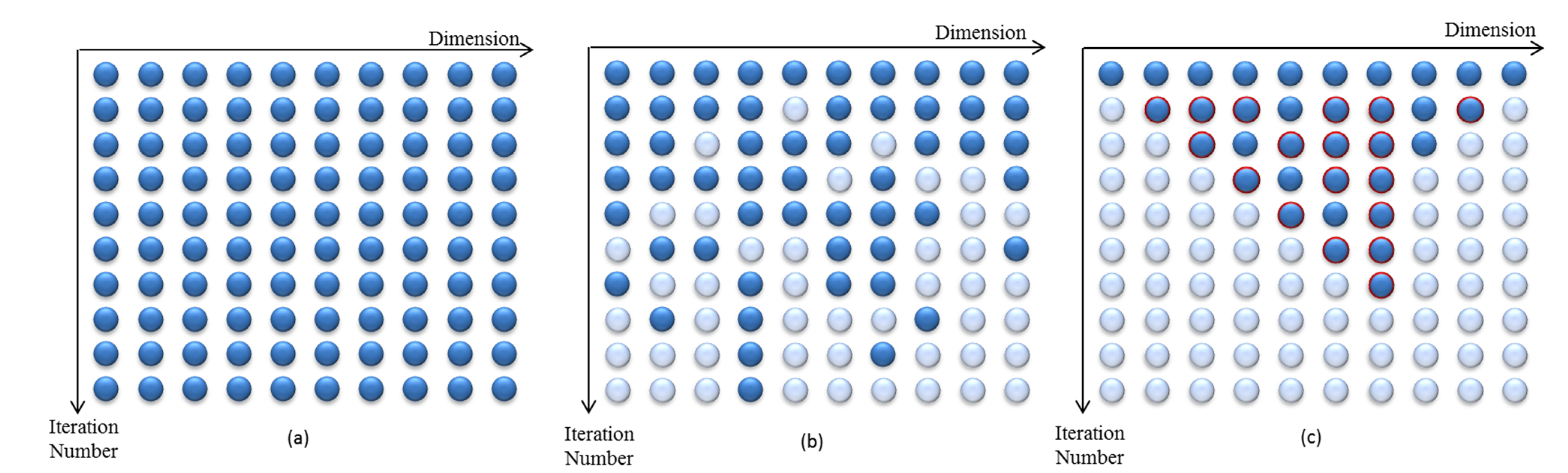
2.2. Heuristic Dynamically Dimensioned Search with Sensitivity Information

The regular used algorithms adopt equal probability search approach without dimension reduction, e.g., the SCE algorithm. The DDS algorithm could select dimensions to search randomly with a function of iteration count, and the number of selected dimensions is decreasing gradually with the increase of iteration count. Similar to the DDS algorithm, covariance matrix adaptation (CMA) and a multi-algorithm, genetically adaptive multi-objective (AMALGAM) algorithms could create the number of offspring points self-adaptively based on experiences, and all the points are searched with the same probabilities [33,34,35,36]. Heuristic dynamically dimensional search with sensitivity information (HDDS-S) improves the equal probability random search with dimension reduction in the DDS, CMA and AMALGAM algorithms, realizing the non-uniform probability search with the changing sensitivity of different dimensions to the objectives. The search approaches of different algorithms are shown in Figure 1.

Figure 1. The search approaches of different algorithms. (a) Equal probability search approach without dimension reduction; (b) Equal probability search approach with dimension reduction; (c) Non-uniform probability search with dimension reduction.

Figure 1. The search approaches of different algorithms. (a) Equal probability search approach without dimension reduction; (b) Equal probability search approach with dimension reduction; (c) Non-uniform probability search with dimension reduction.

Because the number of decision variables that need to be optimized for improving the quality of solutions is decreasing as the values of decision variables approach their best values gradually, the changing process of decision variable sensitivity works on two principles: (1) the sensitivity of decision variable reduces with the increase of decision variables selected for searching on each iteration; (2) the sensitivity of decision variables is continuously cumulative with the increase of iteration number.

In the HDDS-S algorithm, to reflect the two principles, firstly, the sensitivity of each decision variable could be calculated as:

$$\{\begin{array}{c}{s}_{i,j}=1/n_j x_i\in X_j\\ s_{i,j} =0 x_i\notin X_j\end{array}$$

(3)

where $s_{i,j}$ is the sensitivity of decision variable $x_i\left(i=1,\cdots ,D\right)$ on iteration $j\left(j=1,\cdots ,N\right)$, $n_j$ is the number of decision variables selected for searching on iteration $j$, $X_j$ is the collection of decision variables selected for searching on iteration $j$, $D$ and $N$ are the total number of decision variables and iterations respectively.

Secondly, the cumulative sensitivity of decision variable could be calculated as:

$$s{c}_{i,j}={{\displaystyle \sum }}_{l=1}^j\left(N-j+l\right)/m\times s_{i,l}$$

(4)

where $s{c}_{i,j}$ is the cumulative sensitivity of decision variable $x_i$ from $1$ to iteration $j$.

Similar to the DDS algorithm, the HDDS-S algorithm could search from global to local space with a reduced number of dimensions. However, instead of the reducing probability being distributed to each decision variable equally in the DDS algorithm, the non-uniform probability is assigned to each decision variable on the basis of its changing sensitivity to the optimization objectives in the HDDS-S algorithm. The probability of choosing a decision variable to search based on its cumulative sensitivity could be calculated as:

$$P\left(i,j+1\right)=\left(1-ln\left(j\right)/ln\left(N\right)\right)\times \left(\left(s{c}_{i,j}-s{c}_j^{min}\right)/\left(s{c}_j^{max}-s{c}_j^{min}\right)\right)$$

(5)

where $P\left(i,j+1\right)$ is the probability of choosing decision variable $x_i$ to search on iteration $j+1$, $s{c}_j^{max}$ and $s{c}_j^{min}$ are the maximum and minimum cumulative sensitivity values among all decision variables from $0$ to the iteration $j$. The calculation of $P\left(i,j+1\right)$ reflects the dynamic adjustment of decision variable search strategy, that is, the non-uniform probability search with the changing sensitivity of different dimensions to the objectives.

Therefore, the HDDS-S algorithm has the following characteristics: firstly, changing of the sensitivity matrix of multi-dimension parameters (decision variables) and cumulative sensitivity of each parameter are updated dynamically during the process of optimization according to the relationship between dimension selection and optimizing efficiency; secondly, the probability of choosing each parameter to optimize is calculated according to its cumulative sensitivity; finally, the optimization strategy of choosing parameters with non-uniform probability during the process of parameter optimization is realized to improve convergence rate and optimization efficiency. Additionally, similar to the DDS algorithm, the only algorithm parameter to set in the HDDS-S algorithm is the scalar neighbourhood size perturbation that defines the random perturbation size standard deviation as a fraction of the decision variable range. Tolson and Shoemaker [32] recommended the value of $\text{ r}$ parameter as $0.2$ (and used in this study) because this yields a sampling range that practically spans the normalized decision variable range for a current decision variable value halfway between the minimum and maximum.

The complete HDDS-S algorithm pseudo-code for minimization can be seen in the Appendix Pseudo-code of HDDS-S.

3. Model Description and Study Area

Almost all river basin models contain effective physical and/or conceptual model parameters that are either difficult or impossible to directly measure. Optimization algorithms could be used to automate the calibration, i.e., automatic calibration is defined as an optimization algorithm-based search for a set of river basin model parameter values that minimize the model prediction errors relative to available measured data for the system being modeled process. Tolson and Shoemaker [32] compared the performance of the DDS algorithm to that of the SCE algorithm, which is currently one of the most commonly applied algorithms for automatic calibration of river basin models, with multiple optimization test functions as well as real and synthetic SWAT2000 model automatic calibration formulations. In that study, numerical results demonstrate that the DDS algorithm is a more computationally efficient and robust optimization algorithm than the SCE algorithm in the context of river basin model automatic calibration. Therefore, the HDDS-S algorithm developed on the basis of DDS is evaluated by comparing its performance with the DDS algorithm on a river basin model calibration problem in this paper.

Meanwhile, river basin simulation is closely related to multi-reservoir optimal operation. Firstly, the future runoff series under the changing conditions could be generated on the basis of the law of hydrologic cycle evolution, which could be explored with river basin model effectively, e.g., SWAT model. Secondly, the future runoff series need to be used as the inputs of the multi-reservoir operation model to explore the impacts of changing conditions on multi-reservoir operation, determine the operation rules, and assist in making multi-reservoir optimal operation decisions under changing conditions. As with river basin simulation, multi-reservoir optimal operation has been critical for river basin management; the multi-reservoir operation model contains large number of decision variables to be calibrated, i.e., large number of the curves and the number of time periods, which increases the complexity and problem, and poses a significant challenge for most optimization tools currently available [9,10,11,12,13,14]. To evaluate the universality of the HDDS-S algorithm in river basin management, the HDDS-S algorithm is also evaluated by comparing its performance with the DDS algorithm on a multi-reservoir optimal operation problem in this paper.

Two cases are used to extensively test our new HDDS-S algorithm against the DDS algorithm in this paper: (1) the river basin model calibration for Tang-Wang River Basin; and (2) the optimal operation for the DHF-GYG-SW multi-reservoir. The main difference between the multi-reservoir operation model and river basin model is that the decision variables in multi-reservoir operation models are reservoir operation rule curves, which consist of a series of storage volumes or levels at different periods, and the aim of multi-reservoir optimal operation is to establish reservoir operation rule curves at the planning/design stage and provide long-term operation guidelines for reservoir managers to meet expected water demands [37,38,39]. Therefore, the decision variables, which will be optimized in the two optimization problems, are parameters of the river basin model and multi-reservoir optimal operation model, and the dimension being varied is the number of model parameter values being changed to generate a new search neighbourhood.

3.1. Model Description

3.1.1. River Basin Model

Overview of the SWAT Model

The SWAT model is a catchment-scale semi-distributed river basin model developed by the Agricultural Research Service of the United States Department of Agriculture; its detailed description can be seen in many references, such as [40,41]. The SWAT model can be run at a daily time step when the Soil Conservation Service (SCS) curve number method is used to calculate surface runoff, and it is not designed to accurately simulate detailed, single-event flood routing. In this paper, the river basin model calibration problem is formulated based on the set of the SWAT2005 flow-related parameters, which impact snowmelt, surface runoff, groundwater, and lateral flow simulation.

Because SWAT is a semi-distributed river basin model and Hydrological Responding Units (HRUs) divided with geographic information are its basic units, some parameters are not regarded as spatial variables but rather constant values across all spatial units and some other parameters are spatially varied among different HRUs. For example, those parameters related to snowmelt have constant values in all spatial units, and could be calibrated one by one. However, some parameters, such as SCS curve numbers, could be assigned different values for different spatial units, which significantly increase the complexity and computational model requirement of parameter calibration. In this paper, a single factor is used to represent spatial variation, by increasing or decreasing spatially varying parameter values from their base or default values. For spatially varied parameter, this approach maintains the relative differences in the base or default parameter values assigned to different spatial units.

The flow-related parameters of the SWAT model and their ranges are listed in Table 1, where the parameter ranges are based mainly on the default ranges in the SWAT2005 model documentation.

Table 1. Parameter list.

No.	Name	Brief Description (units)	Minimum	Maximum
1	SFTMP	snow fall temperature (°C)	−5	5
2	SMTMP	snowmelt temperature threshold (°C)	−5	5
3	SMFMX	melt factor for snow on June 21 (mm/°C)	1.5	8
4	TIMP	snowpack temperature lag factor	0.01	1
5	ESCO	soil evaporation compensation factor	0.001	1
6	SURLAG	surface runoff lag coefficient	1	24
7	GW_DELAY	groundwater delay time (days)	0.001	500
8	ALPHA_BF	base flow alpha factor	0.001	1
9	GWQMN	threshold groundwater depth for return flow (mm)	0.001	500
10	LAT_TTIME	lateral flow traveltime (days)	0.001	180
11	CN2 a	SCS runoff curve number multiplicative factor for moisture condition II	0.75	1.25

Note: ^a Parameters are multiplicative factors used to adjust the spatial variation across all model units.

Table 1. Parameter list.

No.	Name	Brief Description (units)	Minimum	Maximum
1	SFTMP	snow fall temperature (°C)	−5	5
2	SMTMP	snowmelt temperature threshold (°C)	−5	5
3	SMFMX	melt factor for snow on June 21 (mm/°C)	1.5	8
4	TIMP	snowpack temperature lag factor	0.01	1
5	ESCO	soil evaporation compensation factor	0.001	1
6	SURLAG	surface runoff lag coefficient	1	24
7	GW_DELAY	groundwater delay time (days)	0.001	500
8	ALPHA_BF	base flow alpha factor	0.001	1
9	GWQMN	threshold groundwater depth for return flow (mm)	0.001	500
10	LAT_TTIME	lateral flow traveltime (days)	0.001	180
11	CN2 a	SCS runoff curve number multiplicative factor for moisture condition II	0.75	1.25

Note: ^a Parameters are multiplicative factors used to adjust the spatial variation across all model units.

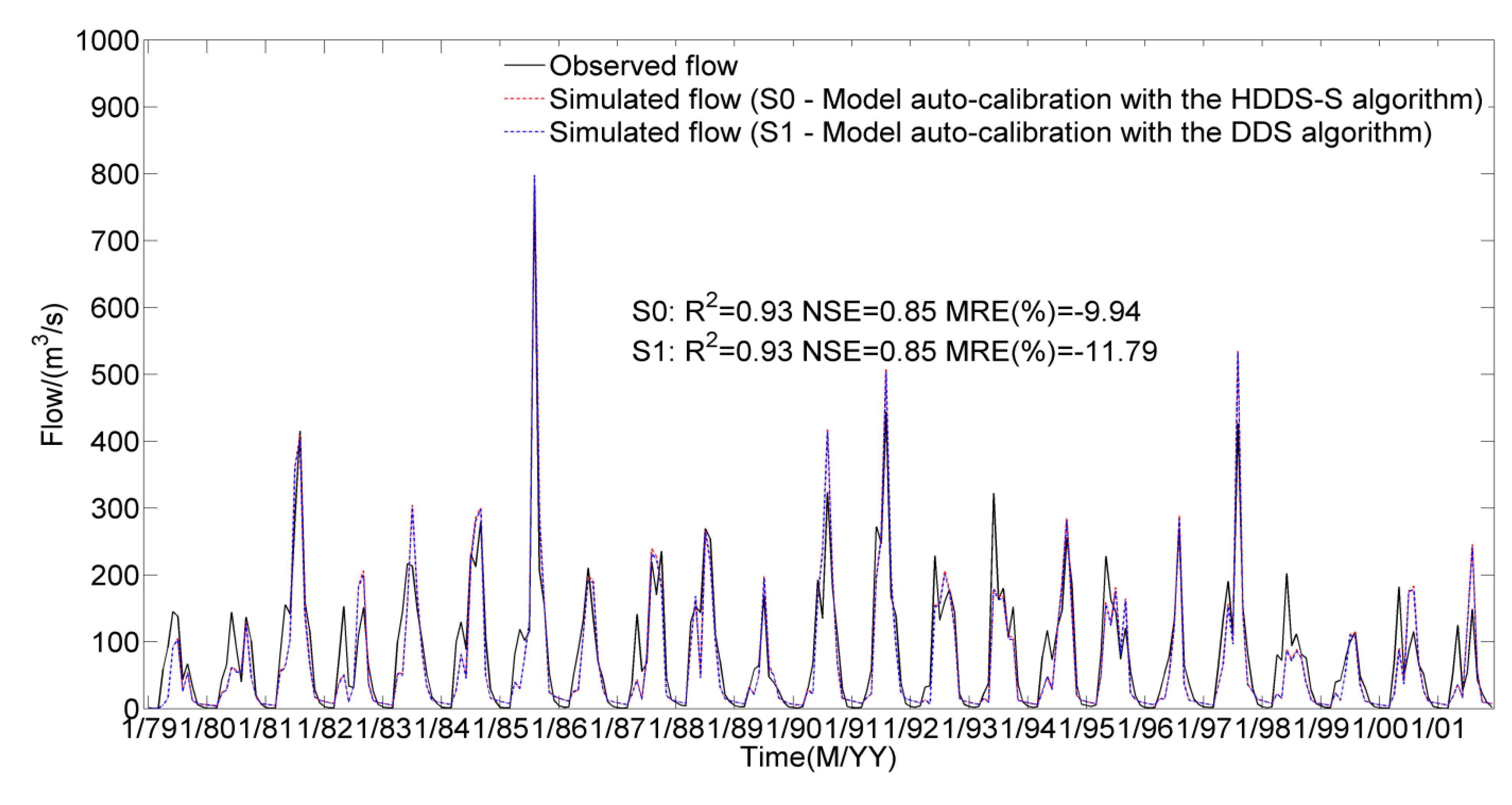
Evaluation Criterion and Objective Function

The mean relative error ($MRE$), the coefficient of determination ($R^2$), and the Nash–Sutcliffe efficiency ($NSE$) are used to evaluate the simulated streamflows with the observed streamflows.

$MRE$ is computed according to Equation (6):

$$MRE=\left(\overline{Q_p}-\overline{Q_t}\right)/\overline{Q_t}\times 100\%$$

(6)

where $\overline{Q_p}$ and $\overline{Q_t}$ are the means of the simulated streamflows and the observed streamflows, respectively. “$MRE$ values of $0$ indicate a perfect fit. Positive values indicate model overestimation bias, and negative values indicate model underestimation bias [42].”

$R^2$ is computed according to Equation (7):

$$R^2={{\displaystyle \sum }}_{i=1}^n\left(Q_{pi}-\overline{Q_p}\right)\left(Q_{ti}-\overline{Q_t}\right)/\sqrt{{{\displaystyle \sum }}_{i=1}^n{\left(Q_{pi}-\overline{Q_p}\right)}^2{{\displaystyle \sum }}_{i=1}^n{\left(Q_{ti}-\overline{Q_t}\right)}^2}$$

(7)

where $Q_{pi}$ is the $i$th simulated value for the streamflows; $Q_{ti}$ is the $i$th observation for the streamflows; and $n$ is the total number of observations. “$R^2$ describes the portion of the variance in measured data explained by the model. $R^2$ ranges from $0$ to $1$, with lower values indicating more error variance, and typically $R^2=1$ is considered the optimal value [43].”

$NSE$ is computed according to Equation (8):

$$NSE=1-{{\displaystyle \sum }}_{i=1}^n{\left(Q_{pi}-Q_{ti}\right)}^2/{{\displaystyle \sum }}_{i=1}^n{\left(Q_{ti}-\overline{Q_t}\right)}^2$$

(8)

The $NSE$ ranges between $-\infty$ and 1.0, with $NSE=1.0$ as the optimal value. According to Luo et al. [44], values between 0.0 and 1.0 are generally viewed as acceptable levels of performance, whereas a value less than 0.0 means that the mean observed value is a better predictor than the simulated value, which indicates unacceptable performance.

To evaluate the HDDS-S algorithm by comparing its performance with that of the DDS algorithm on river basin model calibration, the sum of squared differences between the simulated streamflows and the observed streamflows is used as the objective function, which is shown in Equation (9):

$$SSE={{\displaystyle \sum }}_{i=1}^n{\left(Q_{pi}-Q_{ti}\right)}^2$$

(9)

where $SSE$ is the sum of squared differences between the simulated streamflows and the observed stream flows.

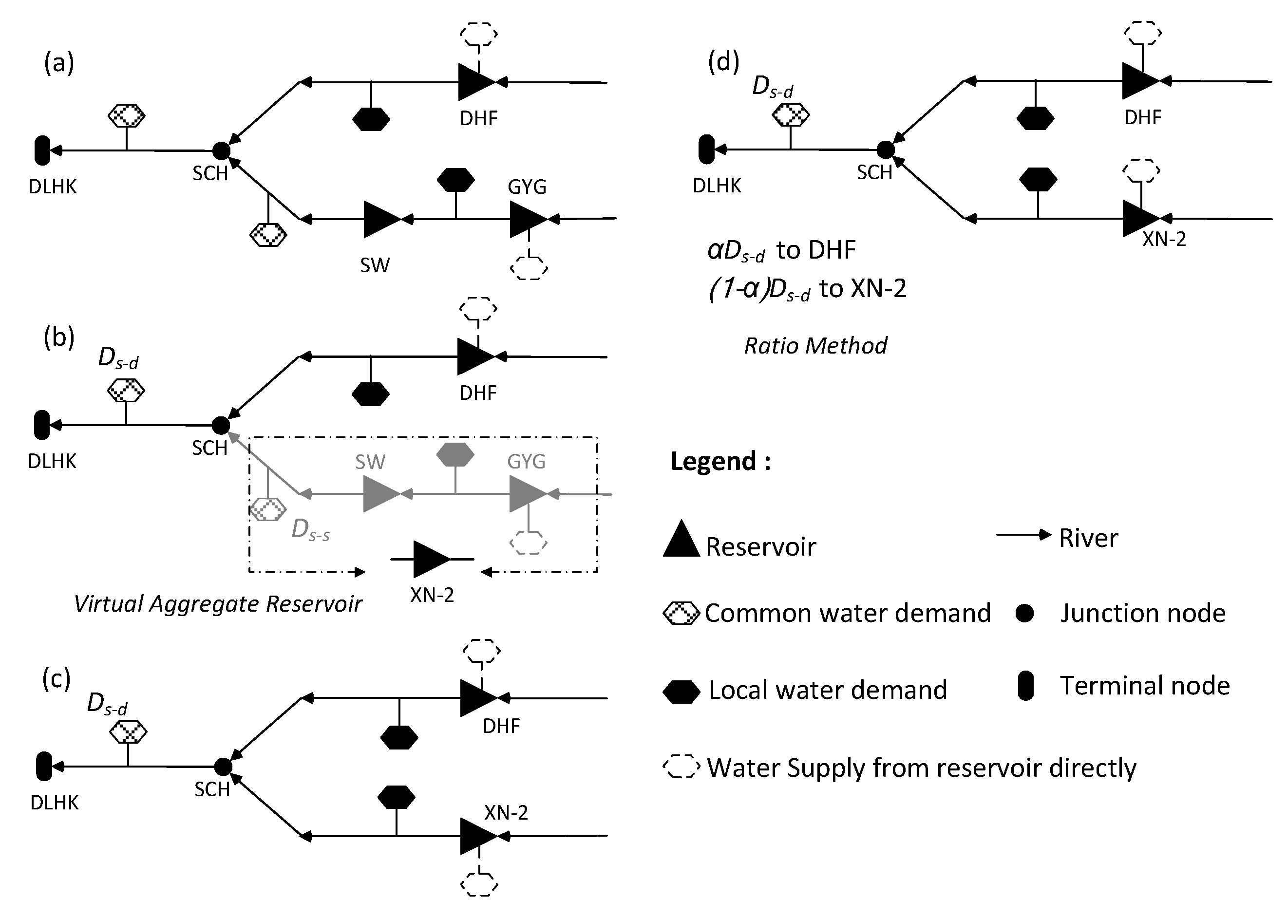
3.1.2. Multi-Reservoir Optimal Operation Model

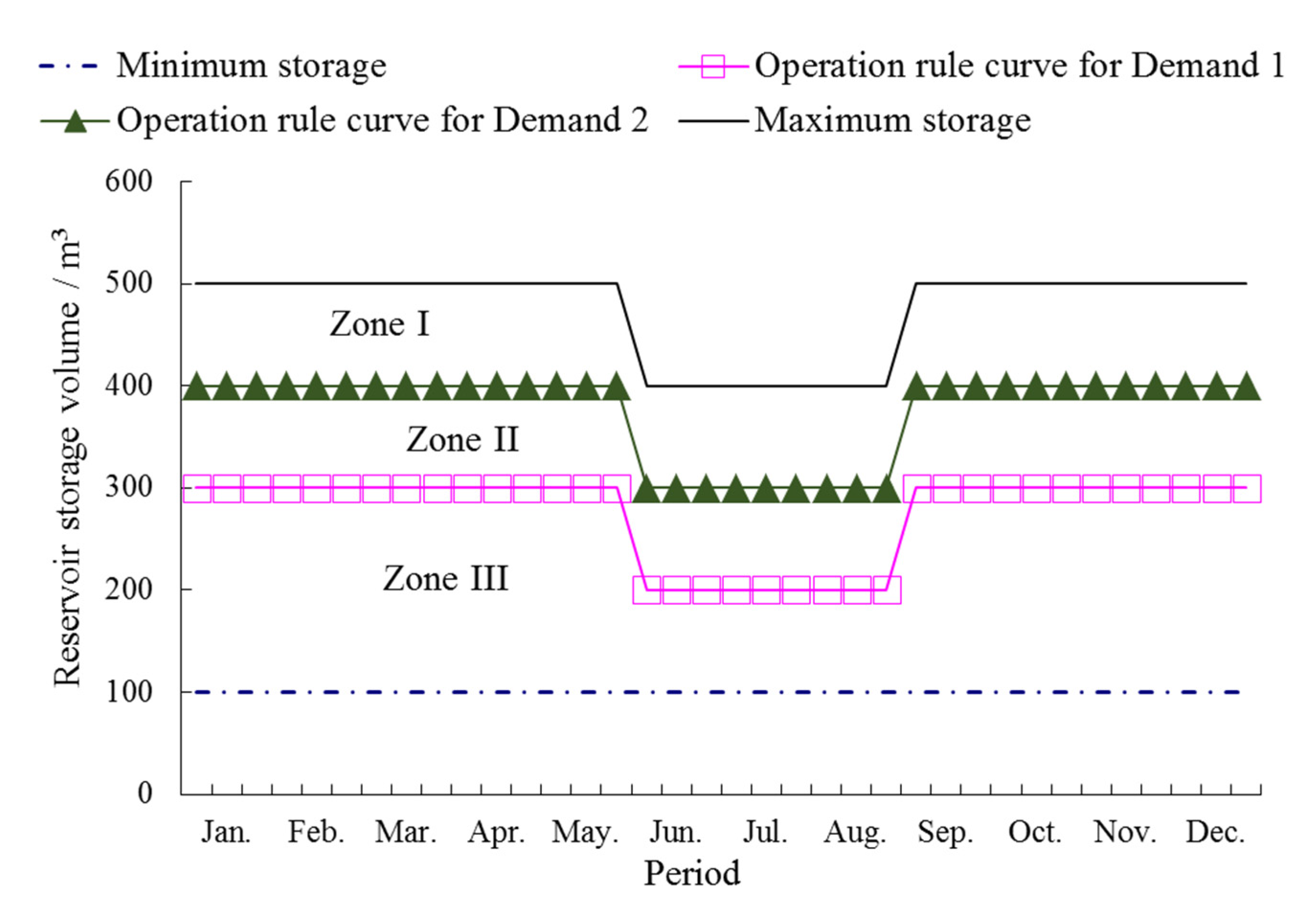
Multi-Reservoir Operation Rule

Multi-reservoir operation rule consists of operation rule curves and rationing factors for each water demand. Details of the operation rule curves and their corresponding water supply rationing factors are illustrated in Figure 2 and Table 2. The forms of reservoir operation rule curves based on 36 10-day periods are shown schematically in Figure 2. The operation rule curves are defined according to reservoir storage, that is, the dynamic water storage of the reservoir is taken as the single, influential factor for reservoir operation.

Figure 2. Reservoir operational rule curves.

Figure 2. Reservoir operational rule curves.

In this paper, the active water storage of reservoir is divided into three parts, zone I, zone II and zone III, by two operation rule curves for industrial (D1) and agricultural (D2) demands. Each of the water demands has a related rule curve and a rationing factor. Because different kinds of water demands require different reliabilities and different degrees of priority in practice, the rationing factors usually have different values. For example, assume water rationing factor is α₁ for the operation rule curve for industrial demand (D1) in Figure 2. When the water storage of the reservoir lies in zone I or zone II, water demand D1 is fully met, i.e., the amount of water supply is D1; when the water storage of reservoir is in zone III, the amount of water supply is calculated by applying the water rationing factor, i.e., α₁× D1.

Table 2. Operation rule implied by rule curves.

Reservoir Storage	Water Supply for Each Demand
	Demand 1 (D1)	Demand 2 (D2)
Zone I	D1	D2
Zone II	D1	α2× D2
Zone III	α1× D1	α2× D2
Rationing factor	α1	α2

Table 2. Operation rule implied by rule curves.

Reservoir Storage	Water Supply for Each Demand
	Demand 1 (D1)	Demand 2 (D2)
Zone I	D1	D2
Zone II	D1	α2× D2
Zone III	α1× D1	α2× D2
Rationing factor	α1	α2

Multi-Reservoir Operation Model

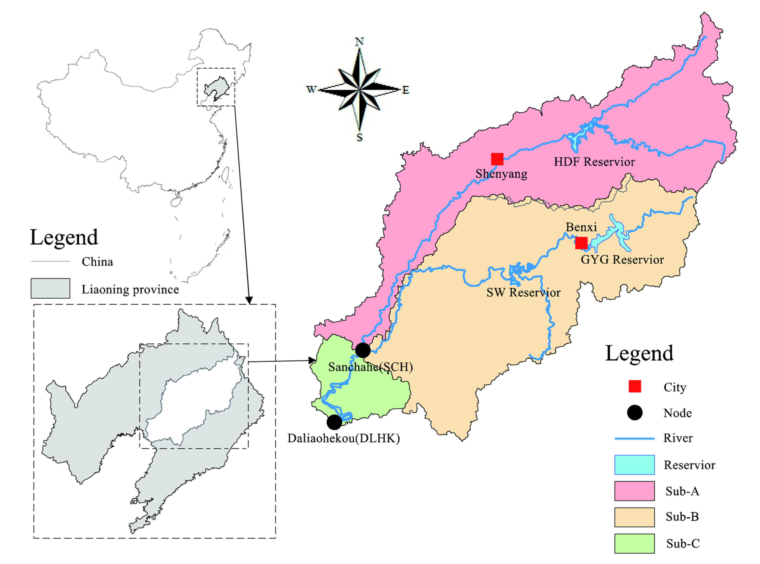
The multi-reservoir optimal operation problem is formulated as a single-objective optimization problem, where decision variables are the water storages at different periods on different operation curves, including industrial and agricultural curves of XN-2 (the virtual reservoir which GYG and SW reservoirs are aggregated into) and DHF reservoirs. Meanwhile, the operation for the entire system should meet the guaranteed rate of each water demand, i.e., the guaranteed water-supply rate of industry and agriculture are above 95% and 50%, respectively. The guaranteed rate of each water demand can be calculated by statistics from the operation result, shown in Equation (10):

$$G{R}_i\left(x\right)=\frac{NT{G}_i}{N{T}_i+1}$$

(10)

where $x$ is the vector of decision variables, i.e., the water storages at different periods on an operation rule curve; $G{R}_i$ is the guaranteed rate for water demand $i$ (industrial water demand when $i=1$, agricultural water demand when $i=2$), which measures the frequency of water demand being satisfied during entire time periods and is used as an indicator to reflect water supply capacity of the system; $N{T}_i$ is the entire operation period for demand $i$ (industrial demand when $i=1$, agricultural demand when $i=2$); similar to $N{T}_i$, $NT{G}_i$ is the time period when water demand $i$ is being satisfied.

Additionally, the number of depth damages, which indicate that the reservoir water storage has been lowered to dead water storage, should be as few as possible during the operation for the entire system. Similarly, the number of depth damages could be calculated by statistics from the operation result.

In this paper, the objectives are set to minimize the number of depth damages, ans improve the guaranteed rate of each water demand during the operation for the entire water supply system:

$$\begin{gathered} minf\left(x\right)=1-{{\displaystyle \sum }}_{i=1}^m{{\displaystyle \sum }}_{j=1}^{n}G{R}_{i,j}+{{\displaystyle \sum }}_{i=1}^m{{\displaystyle \sum }}_{j=1}^{n}N{D}_{i,j} \\ s.t. G{R}_{1,j}\left(x\right)\ge 95\% \\ G{R}_{2,j}\left(x\right)\ge 50\% \end{gathered}$$

(11)

where $G{R}_{i,j}$ is the guaranteed rate for water demand $i$ in subsystem $j$ (Sub A when $j=1$, Sub B when $j=2$, and Sub C when $j=3$); similarly, $N{D}_{i,j}$ is the number of depth damages for water demand $i$ in subsystem $j$.

For the multi-reservoir operation optimization problem, the mass balance equations are:

$$S_{t+1}-S_t=I_t-R_t-S{U}_t-E_t$$

(12)

$$R_t=g\left(x\right), S{U}_t=k\left(x\right), E_t=e\left(x\right)$$

(13)

$$S{T}_t^{min}\le S_t\le S{T}_t^{max}, S{T}_t^{min}\le x\le S{T}_t^{max}$$

(14)

where $S_t$ is the initial water storage at the beginning of period $t$; $S_{t+1}$ is the ending water storage at the end of period $t$; $I_t$, $R_t$, $S{U}_t$, and $E_t$ are inflow, delivery for water use, spill and evapotranspiration loss, respectively; and $S{T}_t^{max}$ and $S{T}_t^{min}$ are the maximum and minimum storage, respectively.

3.2. Study Area

3.2.1. Tang-Wang River Basin

The Tang-Wang River is the first level tributary of the left bank of Song-Hua River, China. The total length of the Tang-Wang River is approximately 509 km. Its basin drains an area of 20,383 km². The study area is limited to the upper-middle stream region of the Tang-Wang River above Yixin hydrologic station, herein still referred to as Tang-Wang River Basin. The river basin drains an area of 11,376 km². The basin boundary and associated SWAT model sub-basin boundaries are presented in Figure 3. There are 87 sub-basins defined in the Tang-Wang River Basin, where 16 rain gauges and 1 streamflow gauge are located. Daily Meteorologic data (temperature, solar radiation, weed speed, relative humidity), daily precipitation data and stream flow data used in SWAT Model Calibration for Tang-Wang River Basin are listed in Table 3.

Figure 3. Tang-Wang River Basin.

Figure 3. Tang-Wang River Basin.

Table 3. Hydrometeorological data for Tang-Wang River Basin.

Time Scale	Hydrologic/Meteorologic Element	Station	Period
Daily	Precipitation	16 gauges, such as Dongsheng	1979–2001
	Streamflow	Yixin	1979–2001
	Temperature, relative humidity, weed speed and solar radiation	Yichun	1979–2001

Table 3. Hydrometeorological data for Tang-Wang River Basin.

Time Scale	Hydrologic/Meteorologic Element	Station	Period
Daily	Precipitation	16 gauges, such as Dongsheng	1979–2001
	Streamflow	Yixin	1979–2001
	Temperature, relative humidity, weed speed and solar radiation	Yichun	1979–2001

To evaluate the HDDS-S algorithm by comparing its performance with that of the original DDS algorithm on river basin model calibration, two scenarios are constructed: (1) model auto-calibration with the HDDS-S algorithm; and the (2) model auto-calibration with the DDS algorithm. The Yixin streamflow gauge was chosen as calibration station, and streamflow data from the 1979–2001 period were used to calibrate the model parameters. For each scenario, the first two months (January and February) are used as a warm up period for model simulation. The rest of the time periods in each scenario are used to assess the model’s performance in the parameter calibration process.

3.2.2. DHF-GYG-SW Multi-Reservoir

This paper use thes DHF-GYG-SW multi-reservoir located in Huntai Basin as a case study, which consists of the Dahuofang reservoir (DHF), Guanyinge reservoir (GYG), and Shenwo reservoir (SW). Huntai basin, including Hun River and Taizi River, is located in a rapidly urbanizing region of Northeast China (Figure 4).

Figure 4. The location of the adopted water supply multi-reservoir.

Figure 4. The location of the adopted water supply multi-reservoir.

DHF is a carry-over storage and is located in the trunk Stream of Hun River. It drains an area of 5437 km², and the total length of the Hun River is approximately 169 km within the basin. GYG and SW are cascade reservoirs and located in the trunk stream of the Taizi River. GYG is a carry-over storage and drains an area of 2795 km², while SW drains an area of 6175 km² with incomplete year regulation performance. The reservoir characteristics, annual average inflow and water supply tasks are illustrated in Table 4.

Table 4. Reservoir characteristics and tasks of water supply.

Reservoir	Minimum Capacity (108 m3)	Active Capacity (108 m3)		Annual Average Inflow (108 m3)	Tasks of Water Supply
		Drought Season	Flood Season
DHF	1.34	14.30	10.00	15.70	(2) (5)
GYG	0.35	14.20	14.20	11.10	(1) (3) (4) (5)
SW	0.35	5.43	2.14	12.80	(4) (5)

Notes: Indicate: (1) industrial water supply from reservoir directly; (2) agricultural water supply for DHF-SCH (DHF-Sanchahe) interval; (3) industrial water supply for GYG-SW interval; (4) agricultural and industrial water supply for SW-SCH (SW-Sanchahe) interval; (5) agricultural and industrial water supply for SW-DLHK (SW-Daliaohekou) interval.

Table 4. Reservoir characteristics and tasks of water supply.

Reservoir	Minimum Capacity (108 m3)	Active Capacity (108 m3)		Annual Average Inflow (108 m3)	Tasks of Water Supply
		Drought Season	Flood Season
DHF	1.34	14.30	10.00	15.70	(2) (5)
GYG	0.35	14.20	14.20	11.10	(1) (3) (4) (5)
SW	0.35	5.43	2.14	12.80	(4) (5)

Notes: Indicate: (1) industrial water supply from reservoir directly; (2) agricultural water supply for DHF-SCH (DHF-Sanchahe) interval; (3) industrial water supply for GYG-SW interval; (4) agricultural and industrial water supply for SW-SCH (SW-Sanchahe) interval; (5) agricultural and industrial water supply for SW-DLHK (SW-Daliaohekou) interval.

The whole multi-reservoir system consists of three parts: subsystem A (Sub-A), which contains DHF and DHF-Sanchahe (SCH) interval; subsystem B (Sub-B), which contains GYG, GYG-SW interval, SW reservoir, and SW-SCH interval; and subsystem C (Sub-C), which contains SCH-Daliaohekou (DLHK) interval. The corresponding topological structure is generated, as shown in Figure 5a. Sub-A is supplied with water from DHF and uses DHF operation rules to decide how to supply water to each user in this subsystem. Sub-B is supplied with water from GYG and SW, which constitute cascade reservoirs and so are aggregated into one virtual reservoir (XN-2 reservoir), as shown in Figure 5b. Sub-C is supplied with water from the parallel reservoir, i.e., XN-2 and DHF, the common tasks in Sub-C should be allocated to XN-2 and DHF. The water ratio method is employed to allocate the common tasks in Sub-C, which is a simple and efficient method shown in Figure 5c,d.

Figure 5. Reservoir aggregation and common water supply task allocation, (a) initial topological structure; (b) formation of virtual aggregate reservoir; (c) final topological structure after reservoir aggregation; (d) common water supply task allocation in the final topological structure.

Figure 5. Reservoir aggregation and common water supply task allocation, (a) initial topological structure; (b) formation of virtual aggregate reservoir; (c) final topological structure after reservoir aggregation; (d) common water supply task allocation in the final topological structure.

The calculation of water division coefficient $\text{α}$ is shown in Equations (15)–(17):

$$\text{α}=SI{D}_{DHF,t}/\left(SI{D}_{DHF,t}+SI{D}_{XN-2,t}\right)$$

(15)

$$SI{D}_{DHF,t}=S_{DHF,t}+I_{DHF,t}-D_{DHF,t}$$

(16)

$$SI{D}_{XN-2,t}=S_{XN-2,t}+I_{XN-2,t}-D_{XN-2,t}$$

(17)

where $S_{DHF,t}$ is the initial water storage of DHF at the beginning of period $t$; $I_{DHF,t}$ and $D_{DHF,t}$ are the inflow into DHF and water supply from DHF during the period $t$, respectively; $S_{XN-2,t}$ is the initial water storage of virtual aggregate reservoir XN-2 at the beginning of period $t$, i.e., the sum water storage of GYG and SW; $I_{XN-2,t}$ and $D_{XN-2,t}$ are the inflow into XN-2 and water supply from XN-2 during the period $t$, i.e., the sum inflow into GYG and SW, the sum water supply from GYG and SW, respectively.

4. Applications of the HDDS-S Algorithm and Results

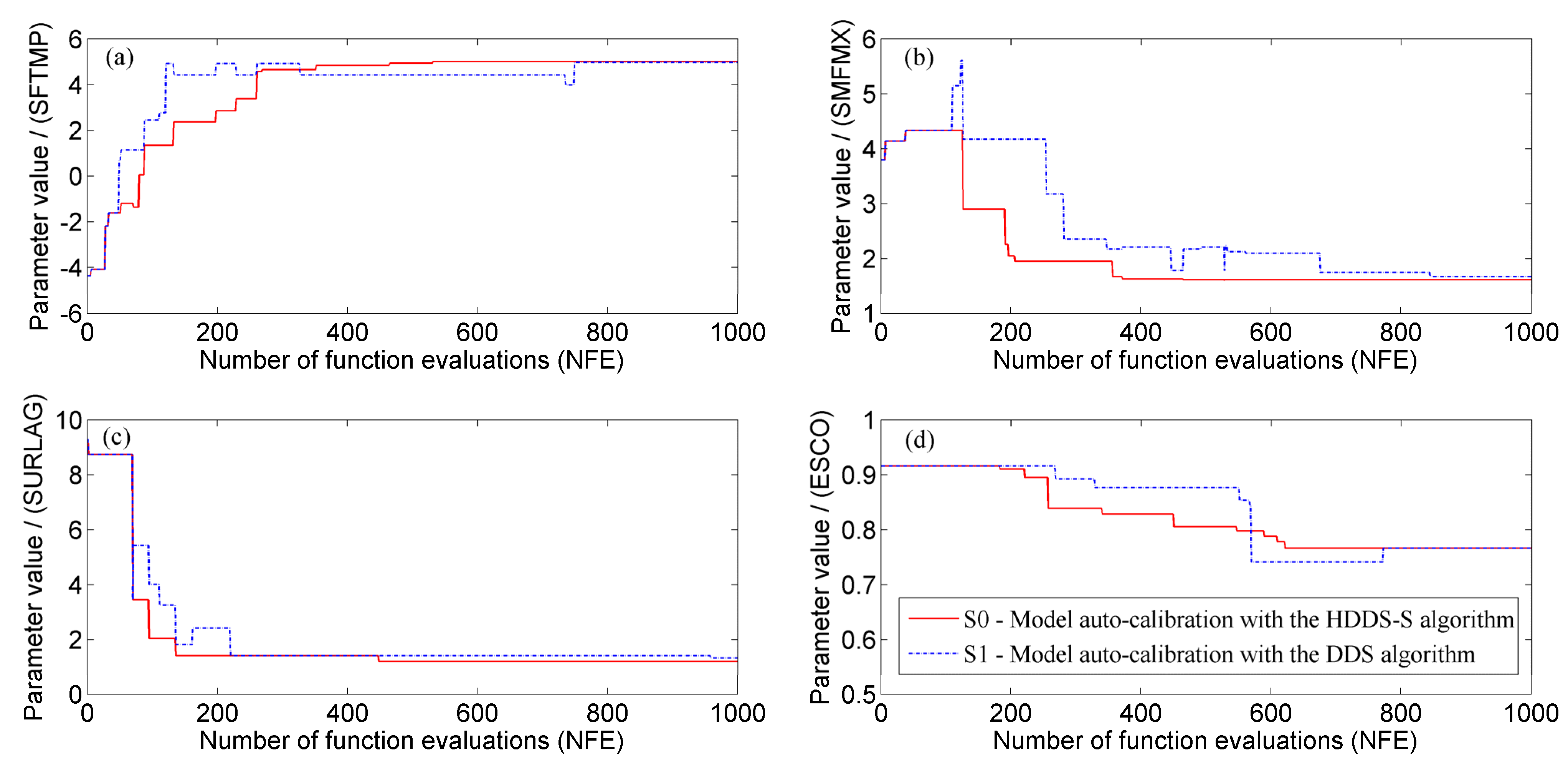
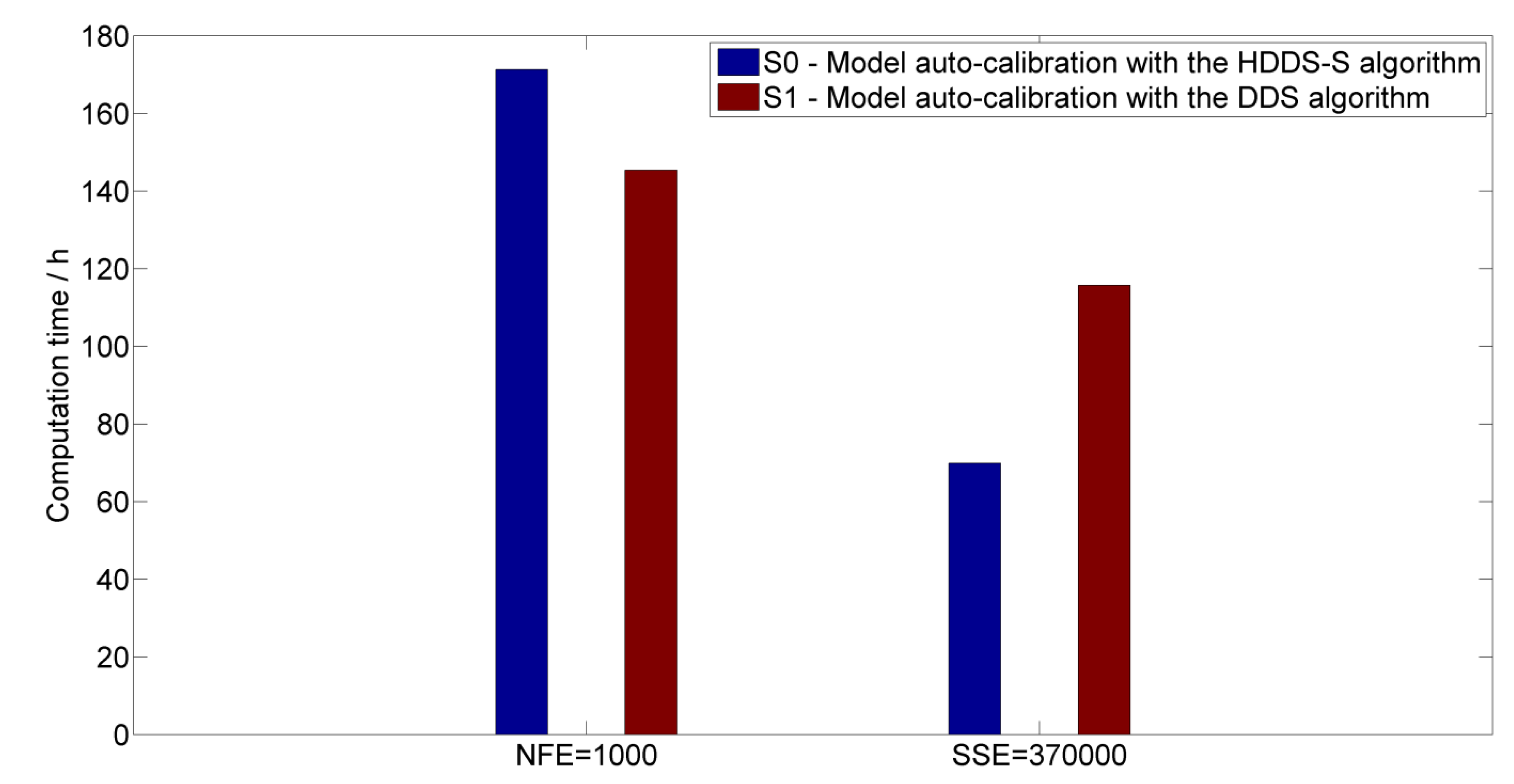
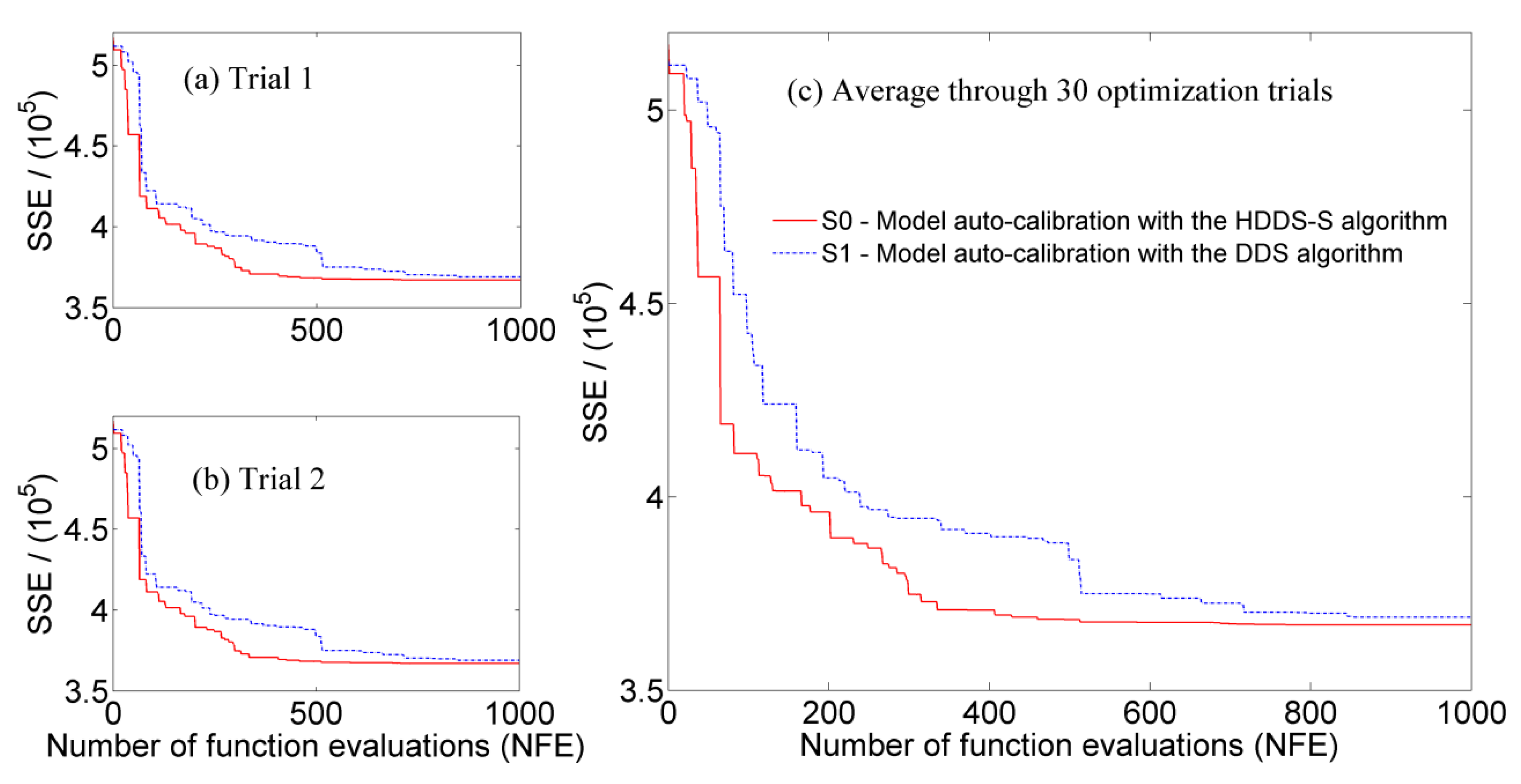
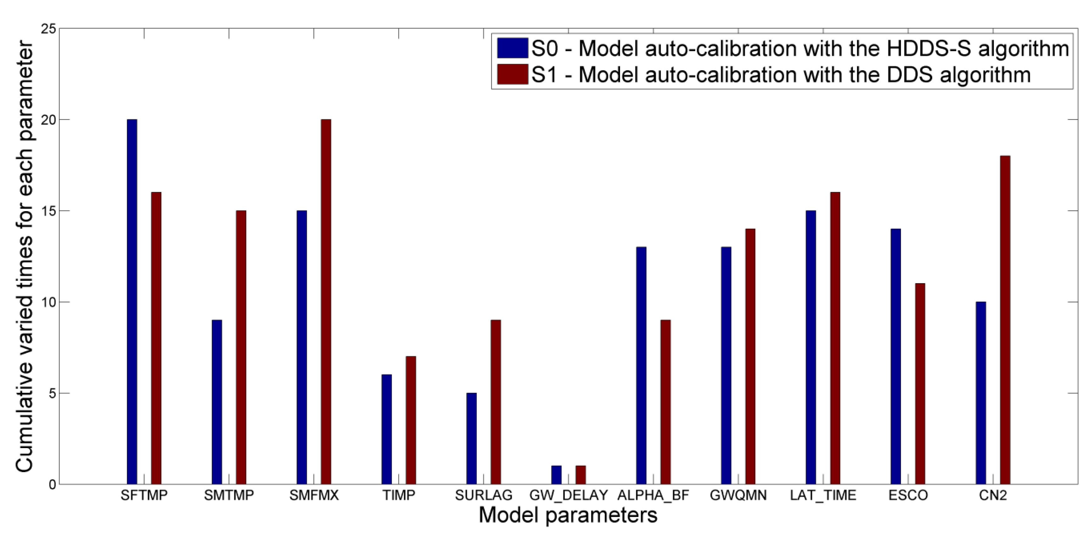
4.1. River Basin Model Calibration

The river basin model calibration problem for the Tang-Wang River Basin is used to validate effectiveness of the new HDDS-S algorithm. The Yixin hydrologic station, located at the outlet of Tang-Wang River Basin, is chosen as the calibration station, and the streamflow data from the 1979–2001 periods are used to calibrate model parameters. Based on the two scenarios S0 and S1, i.e., model auto-calibration with the HDDS-S and DDS algorithms respectively, performances of the two algorithms in the river basin model parameter auto-calibration are evaluated on Intel Core™ 2 Duo, with a 2.66-GHz CPU. In different scenarios, average required computation time under the same number of function evaluations, i.e., $NFE=1000$, or the same simulation accuracy, i.e., $SSE=370,000$, through 30 optimization trials are shown in Figure 6.

Figure 6. Average required computation time under the same number of function evaluations ($NFE=1000$) and the same simulation accuracy ($SSE=370,000$) in different scenarios through 30 optimization trials.

Figure 6. Average required computation time under the same number of function evaluations ($NFE=1000$) and the same simulation accuracy ($SSE=370,000$) in different scenarios through 30 optimization trials.

In different scenarios, average simulation results at the Yixin hydrologic station under the same number of function evaluations, i.e., $NFE=1000$, through 30 optimization trials is shown in Figure 7.

Figure 7. Observed and average simulated monthly streamflows during the period from 1979 to 2001 at the Yixin hydrologic station through 30 optimization trials.

Figure 7. Observed and average simulated monthly streamflows during the period from 1979 to 2001 at the Yixin hydrologic station through 30 optimization trials.

Seen from Figure 6 and Figure 7, under the same number of function evaluations ($NFE=1000$), the average required computation time increases from 145.40 h in the case of the DDS algorithm to 171.32 h in the HDDS-S algorithm. Although the model performance improves from 11.79% ($MRE$) in the case of the DDS algorithm to 9.94% in the HDDS-S algorithm at the Yixin hydrologic station, there is little difference of model performances between the DDS algorithm and the HDDS-S algorithm in terms of the other two evaluation criterions because the simulation results will approximate their optimal values after 1000 function evaluations to a large extent. Under the same simulation accuracy ($SSE=370,000$), the average required computation time reduces from 115.74 h ($NFE=796$) in the case of the DDS algorithm to 69.90 h ($NFE=408$) in the HDDS-S algorithm through 30 optimization trials. Although the average computation time in the case of the HDDS-S algorithm increases due to the additive sensitivity computation of each dimension decision variable compared to the DDS algorithm under the same iteration number, the average computation time in the case of the HDDS-S algorithm reduces greatly compared to the DDS algorithm under the same simulation accuracy.

The performances of the two algorithms in river basin model calibration are evaluated not only from average required computation time under the same number of function evaluations, average required computation time under the same simulation accuracy, and average simulation results at Yixin hydrologic station under the same number of function evaluations, but also from average convergence process of the objective function and average calibration process of model parameters under the same number of function evaluations. Convergence processes of the objective function under the same number of function evaluations ($NFE=1000$) through 30 optimization trials in different scenarios are shown in Figure 8. It is further indicated that due to the consideration of the changing sensitivity information of each dimension decision variable, under the same number of function evaluations, convergence rate of the objective function is improved in the HDDS-S algorithm compared to the DDS algorithm. Additionally, there are few differences of the HDDS-S algorithm convergence processes among different optimization trials, which indicate the reliability and stability of the HDDS-S algorithm in solving model auto-calibration problem.

Under the same number of function evaluations ($NFE=1000$), the average cumulative varied times for each parameter during model auto-calibration process in different scenarios through 30 optimization trials are shown in Figure 9, where the average cumulative varied times in S0 indicate the cumulative sensitivity of each parameter.

Figure 8. Convergence processes of the objective function under the same number of function evaluations ($NFE=1000$) in different scenarios through 30 optimization trials, (a) and (b) convergence processes in two random optimization trials; (c) average convergence process through 30 optimization trials.

Figure 8. Convergence processes of the objective function under the same number of function evaluations ($NFE=1000$) in different scenarios through 30 optimization trials, (a) and (b) convergence processes in two random optimization trials; (c) average convergence process through 30 optimization trials.

Figure 9. Average cumulative varied times for each parameter during model auto-calibration process under the same number of function evaluations ($NFE=1000$) in different scenarios through 30 optimization trials, where the description of each parameter in the x axis could be found in Table 1.

Figure 9. Average cumulative varied times for each parameter during model auto-calibration process under the same number of function evaluations ($NFE=1000$) in different scenarios through 30 optimization trials, where the description of each parameter in the x axis could be found in Table 1.

The average cumulative varied times for each parameter during model auto-calibration process under the same number of function evaluations ($NFE=1000$) through 30 optimization trials are different between the two scenarios, i.e., the DDS algorithm, which selects dimension for perturbation completely at random with a uniform probability, could not reflect the sensitivity information of each parameter. The details are indicated from two aspects.

(1) As indicated in the cumulative varied times in the case of the HDDS-S algorithm, some parameters need to be varied many times due to strong sensitivities, e.g., SFTMP, ALPHA_BF and ESCO. However, the cumulative varied times of these parameters in the DDS algorithm are less.

(2) Similarly, some parameters need to be varied fewer times due to weak sensitivities, e.g., SMTMP, SMFMX, SURLAG and CN2. However, their cumulative varied times in the DDS algorithm are greater than.

Under the same number of function evaluations ($NFE=1000$) through 30 optimization trials, average calibration processes of model parameters SFTMP, SMFMX, SURLAG and ESCO, in different scenarios are shown in Figure 10.

Figure 10. Average calibration process of model parameters under the same iteration number ($NFE=1000$) through 30 optimization trials in different scenarios, (a) SFTMP; (b) SMFMX; (c) SURLAG and (d) ESCO.

Figure 10. Average calibration process of model parameters under the same iteration number ($NFE=1000$) through 30 optimization trials in different scenarios, (a) SFTMP; (b) SMFMX; (c) SURLAG and (d) ESCO.

It is indicated from Figure 9 and Figure 10 that the value of the most sensitive parameter SFTMP needs to be varied through the whole calibration process, while its calibration is stopped when reaching some iteration number in the DDS algorithm. Similarly, the value of some more sensitive parameters, such as ESCO also needs to be varied many times, while it is calibrated with fewer variation times, scatter variation moments and obvious stagnation phenomenon in the DDS algorithm. However, less sensitive parameters SURLAG and SMFMX needs to be varied fewer times, while it is calibrated with more variation times, scatter variation moments and obvious stagnation phenomenon in the DDS algorithm. Therefore, no matter how sensitive these parameters are, they could be calibrated to their optimal values much faster with the HDDS-S algorithm than the DDS algorithm.

River basin model calibration results show that the computation time and efficiency could be improved in the HDDS-S algorithm, including the enhanced convergence rate of objective function, concentrated varied moments, reduced blind variation and stagnation phenomenon, compared to the DDS algorithm. Therefore, the HDDS-S algorithm is more efficient than the DDS algorithm in the river basin model calibration for the specific catchment.

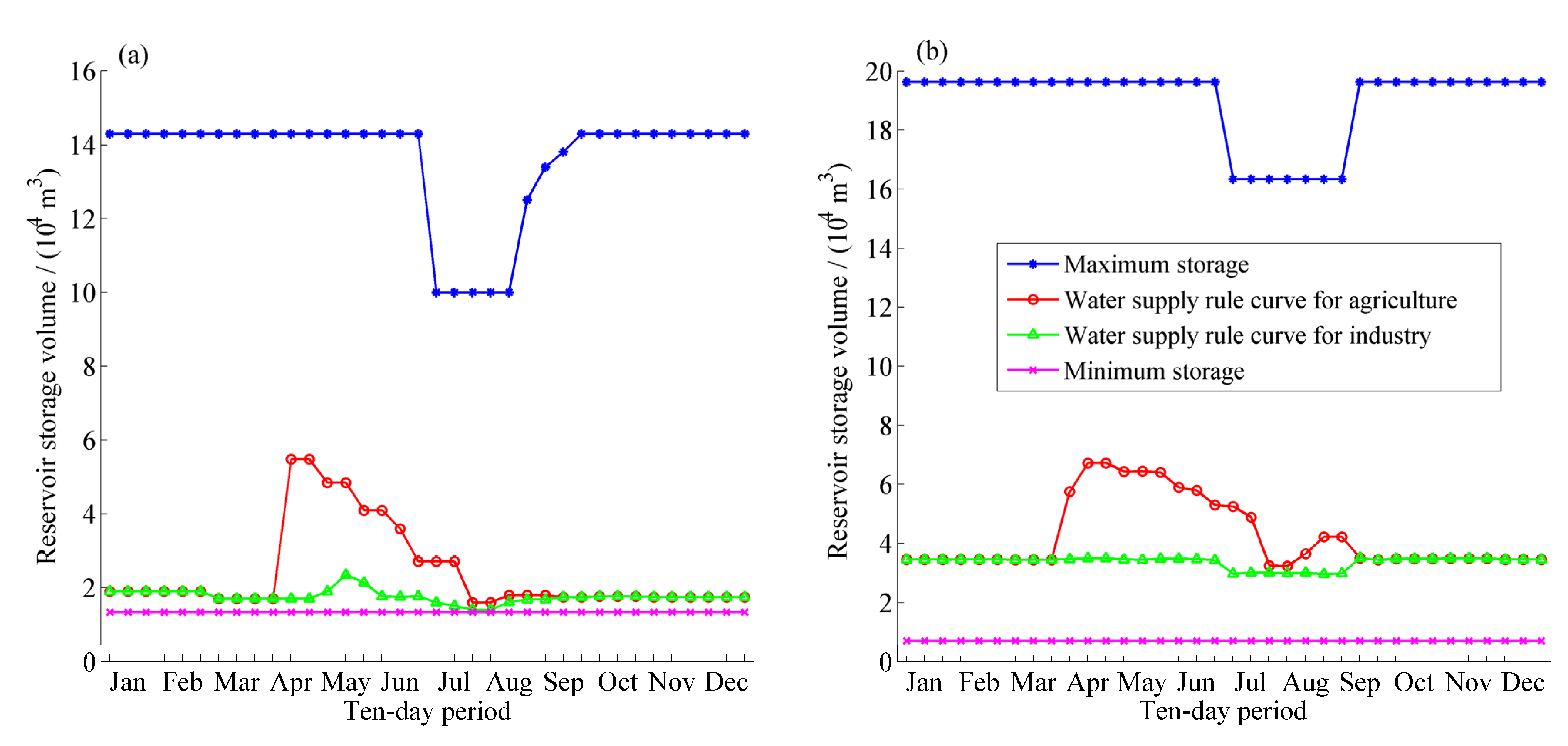
4.2. Multi-Reservoir Optimal Operation

The optimal operation problem for DHF-GYG-SW multi-reservoir is used to evaluate the universality of the HDDS-S algorithm in river basin management. The input data are inflow and water demand data, including the industrial and agricultural water demands in the future planning year, i.e., 2030, and the history inflow from 1956 to 2006. Each calculation year is divided into 24 time periods (with ten days as scheduling horizon from April to September, and a month as scheduling horizon in the remaining months). Since the industrial water supply occurs through the whole year, there are twenty-four decision variables for industrial water supply. The agricultural water supply occurs only during the periods from the second ten-day of April to the first ten-day of September, thus there are fifteen decision variables for agricultural water supply. Therefore, the entire operation system has four rule curves and (24 + 15) × 2 = 78 decision variables in total.

Similarly, based on the two scenarios S0 and S1, i.e., multi-reservoir optimal operation in the case of the HDDS-S algorithm and multi-reservoir optimal operation in the DDS algorithm respectively, average performances of the two algorithms in multi-reservoir optimal operation are evaluated under the same iteration number ($NFE=10,000$) through 30 optimization trials from three aspects, including average required computation time, average objective function value, and average guaranteed water-supply rate on Intel Core™ 2 Duo, with a 2.66-GHz CPU.

First of all, the rationality of operation rules derived after 10,000 function evaluations in one random optimization trial in the case of the HDDS-S algorithm is evaluated, and the joint scheduling charts are presented in Figure 11.

As industrial water demand is more urgent than agricultural water demand, and the agricultural water would be limited primarily when reservoir storage is insufficient, the water supply rule curve for agriculture is above the operation rule curve for industry, as shown in Figure 10. In the scheduling cycle duration, each rule curve decreases before the flood season and then has a different degree of uplift after the flood season. In order to prepare for the large inflow of the summer flood season and to reduce surplus water, the reservoir active storage before the flood season should be lowered and then the number of limited water supply is reduced, i.e., the operation rule curves are decreased before the flood season. After the flood season, when the inflow decreases gradually, in order to ensure that no depth damage happens in dry years, the curves are raised to fill reservoirs as early as possible and the number of limited water supply is increased. In addition, the largest agricultural water use happens from April to May, thus the operation rule curve of agriculture is higher in the duration to conserve water and mitigate potential future shortages for industrial demand in some dry years. Specifically, referred to DHF reservoir, its water supply rule curve for industry falls in the duration from March to April due to spring floods produced by melting snow, meanwhile, its water supply rule curve for industry raises in May because the largest agricultural water use happens from April to May and much water has been supplied to agriculture.

Figure 11. The derived operational rule curves with the HDDS-S algorithm after 10,000 function evaluations in one random optimization trial, (a) DHF reservoir operation rule curve; (b) XN-2 reservoir operation rule curve.

Figure 11. The derived operational rule curves with the HDDS-S algorithm after 10,000 function evaluations in one random optimization trial, (a) DHF reservoir operation rule curve; (b) XN-2 reservoir operation rule curve.

Additionally, the average scheduling results determined by operation rule curves derived with the HDDS-S algorithm after 10,000 function evaluations in 30 random optimization trials are: (1) In Sub A, the guaranteed rate for industrial and agricultural water demands are 95.10% and 75.35% respectively; (2) In Sub B, the guaranteed rate for industrial and agricultural water demands are 95.81% and 75.46% respectively; (3) In Sub C, the guaranteed rate for industrial and agricultural water demands are 96.08% and 62.56% respectively. The average guaranteed rates in all three subsystems meet the requirement, i.e., guaranteed rate for industrial and agricultural water demands exceed 95% and 50% respectively.

Therefore, as mentioned above, the derived operational rule curves of DHF reservoir and XN-2 reservoir in the HDDS-S algorithm and the scheduling results are reasonable.

In different scenarios, under the same number of function evaluations ($NFE=10,000$), average required computation time and objective function value through 30 random optimization trials are shown in Table 5.

Table 5. Average computation time and objective function value under the same iteration number ($NFE=10,000$) through 30 random optimization trials in different scenarios.

Scenario	Objective Function Value	Computation Time/Second
S0	9.13	723.73
S1	25.68	294.37.2

Table 5. Average computation time and objective function value under the same iteration number ($NFE=10,000$) through 30 random optimization trials in different scenarios.

Scenario	Objective Function Value	Computation Time/Second
S0	9.13	723.73
S1	25.68	294.37.2

Under the same number of function evaluations ($NFE=10,000$), though larger differences of average required computation time exist in different scenarios, average objective function value decreases from 25.68 in the DDS algorithm to 9.13 in the HDDS-S algorithm, which improve obviously.

Average guaranteed water-supply rates for all water supply area under the same number of function evaluations ($NFE=10,000$) through 30 random optimization trials in different scenarios are shown in Table 6. Under the same number of function evaluations ($NFE=10,000$), though few differences of average guaranteed rate for industrial water demand exist in different scenarios, i.e., the guaranteed rate for industrial water demand in all three subsystems exceed 95%, the average guaranteed rates for agricultural water demand in all three subsystems increase from 67.52%, 64.78% and 50.94% in the DDS algorithm to 75.35%, 75.46% and 62.54% in the HDDS-S algorithm in Sub A, Sub B and Sub C respectively, which improved obviously.

Table 6. Average guaranteed water-supply rate under the same iteration number ($NFE=10,000$) through 30 random optimization trials in different scenarios.

Water Supply Area		Guaranteed Water-Supply Rate (%)
		Industry		Agriculture
		S0	S1	S0	S1
Sub-system	Sub A (DHF subsystem)	95.10	95.06	75.35	67.52
	Sub B (GYG-SW subsystem)	95.81	96.00	75.46	64.78
	Sub C (SCH-DLHK subsystem)	96.08	96.25	62.54	50.94

Table 6. Average guaranteed water-supply rate under the same iteration number ($NFE=10,000$) through 30 random optimization trials in different scenarios.

Water Supply Area		Guaranteed Water-Supply Rate (%)
		Industry		Agriculture
		S0	S1	S0	S1
Sub-system	Sub A (DHF subsystem)	95.10	95.06	75.35	67.52
	Sub B (GYG-SW subsystem)	95.81	96.00	75.46	64.78
	Sub C (SCH-DLHK subsystem)	96.08	96.25	62.54	50.94

Optimal operation of DHF-GYG-SW multi-reservoir results show that the derived operational rule curves of DHF reservoir and XN-2 reservoir and the scheduling results from one random optimization trial are reasonable in the case of the HDDS-S algorithm, while average guaranteed water-supply rates in all subsystems could be improved in the HDDS-S algorithm under the same number of function evaluations ($NFE=10,000$) through 30 random optimization trials compared to the DDS algorithm. Therefore, the HDDS-S algorithm is able to derive good solutions and thus is effective in the specific large multi-reservoir optimal operation.

5. Discussions and Conclusions

The DDS algorithm could automatically refine and update optimal search space, i.e., searches globally at the start of the search and conducts a more localized search as the number of iterations approaches the maximum allowable number of function evaluations, and automatically adjust and exhibit good performance within the user’s timeframe for calibration to obtain a quick and approximate result, which is achieved by dynamically and probabilistically reducing the number of dimensions in the neighborhood and the reducing probability is distributed to each decision variable equally [45,46]. With multiple optimization test functions as well as real and synthetic SWAT2000 model automatic calibration formulations, Tolson and Shoemaker [32] have proved that the DDS algorithm could return good solutions faster than the SCE algorithm within the maximum allowable number of function evaluations.

In this paper, the DDS algorithm is improved with reference to the changing sensitivity information of multi-dimension decision variables, and the HDDS-S algorithm is proposed based on the sensitivity analysis. The HDDS-S algorithm consists of three steps: firstly, the changing sensitivity matrix of multi-dimension parameters and cumulative sensitivity of each parameter are updated dynamically during the process of optimization according to the relationship between dimension selection and optimizing efficiency; secondly, the probability of choosing each parameter is calculated during the process of optimization according to its cumulative sensitivity; finally, the optimization strategy with non-uniform probability of choosing parameters during the process of parameter optimization is realized to improve convergence rate and optimizing efficiency. The HDDS-S algorithm is tested extensively against the DDS algorithm on the river basin model calibration problem for Tang-Wang River Basin in Jilin province, China, and the optimal operation problem for DHF-GYG-SW multi-reservoir in the northeast of China.

In the river basin model calibration problem for Tang-Wang River Basin, although there is little difference of model performances between the DDS algorithm and the HDDS-S algorithm because the simulation results will approximate their optimal values after 1000 function evaluations to a large extent, the average required computation time reduces from 115.74 h ($NFE=796$) in the case of the DDS algorithm, to 69.90 h ($NFE=408$) in the HDDS-S algorithm, through 30 optimization trials under the same simulation accuracy ($SSE=370,000$). Meanwhile, due to the consideration of the changing sensitivity information of each dimension decision variable, under the same iteration number, the convergence rate of the objective function is improved in the HDDS-S algorithm compared to the DDS algorithm, and there are few differences of the HDDS-S algorithm convergence processes among different optimization trials, which indicate the reliability and stability of the HDDS-S algorithm in solving the model auto-calibration problem. Additionally, in the optimal operation problem for the DHF-GYG-SW multi-reservoir, under the same number of function evaluations ($NFE=10,000$), though few differences of average guaranteed rate for industrial water demand exist in different scenarios, i.e., the guaranteed rate for industrial water demand in all three subsystems exceed 95%, the average guaranteed rates for agricultural water demand in all three subsystems increase from 67.52%, 64.78% and 50.94% in the DDS algorithm to 75.35%, 75.46% and 62.54% in the HDDS-S algorithm in Sub A, Sub B and Sub C respectively. Overall, results show that the HDDS-S algorithm could be more efficient and effective than the DDS algorithm in the two specific problems.

Since one algorithm may be better for calibration of the river basin model for only one catchment or one specific multi-reservoir optimal operation, we will choose other catchments and multi-reservoir operation systems with different characteristics including climate, topography and human activities, to examine the performance of the HDDS-S algorithm under different conditions in future studies.

References

1. Labat, D.; Godderis, Y.; Probst, J.L.; Guyot, J.L. Evidence for global runoff increase related to climate warming. Adv. Water Resour. 2004, 27, 631–642. [Google Scholar] [CrossRef] [Green Version]
2. Barnett, T.P.; Pierce, D.W.; Hidalgo, H.G.; Bonfils, C.; Santer, B.D.; Das, T.; Dettinger, M.D. Human-induced changes in the hydrology of the western United States. Science 2008, 319, 1080–1083. [Google Scholar] [CrossRef] [PubMed]
3. Zhang, A.; Zhang, C.; Chu, J.; Fu, G. Study on the human-induced runoff change in Northeast China. J. Hydrol. Eng. 2014. [Google Scholar] [CrossRef]
4. Zhang, A.; Zhang, C.; Fu, G.; Wang, B.; Bao, Z.; Zheng, H. Assessments of impacts of climate change and human activities on runoff with SWAT for the Huifa River Basin, Northeast China. Water Resour. Manag. 2012, 26, 2199–2217. [Google Scholar] [CrossRef]
5. Zhang, C.; Shoemaker, C.A.; Woodbury, J.D.; Cao, M.; Zhu, X. Impact of human activities on stream flow in the Biliu River basin, China. Hydrol. Process. 2013, 27, 2509–2523. [Google Scholar] [CrossRef]
6. Zhang, C.; Zhu, X.; Fu, G.; Zhou, H.; Wang, H. The impacts of climate change on water diversion strategies for a water deficit reservoir. J. Hydroinform. 2013. [Google Scholar] [CrossRef]
7. Zhang, C.; Wang, D.; Wang, G.; Yang, W.; Liu, X. Regional differences in hydrological response to canopy interception schemes in a land surface model. Hydrol. Process. 2014, 28, 2499–2508. [Google Scholar] [CrossRef]
8. Wang, F.; Zhang, C.; Peng, Y.; Zhou, H. Diurnal temperature range variation and its causes in a semiarid region from 1957 to 2006. Int. J. Climatol. 2014, 34, 343–354. [Google Scholar] [CrossRef]
9. Labadie, J.W. Optimal operation of multireservoir systems: State-of-the-art review. J. Water Resour. Plan. Manag. 2004, 130, 93–111. [Google Scholar] [CrossRef]
10. Draper, A.J.; Lund, J.R. Optimal hedging and carryover storage value. J. Water Resour. Plan. Manag. 2004, 130, 83–87. [Google Scholar] [CrossRef]
11. Sadegh, M.; Mahjouri, H.; Kerachian, R. Optimal inter-basin water allocation using crisp and fuzzy Shapley games. Water Resour. Manag. 2010, 24, 2291–2310. [Google Scholar] [CrossRef]
12. Zhang, C.; Wang, G.; Peng, Y.; Tang, G.; Liang, G. A negotiation-based multi-objective, multi-party decision-making model for inter-basin water transfer scheme optimization. Water Resour. Manag. 2012, 26, 4029–4038. [Google Scholar] [CrossRef]
13. Zhao, T.; Zhao, J.; Yang, D. Improved dynamic programming for hydropower reservoir operation. J. Water Resour. Plan. Manag. 2014, 140, 365–374. [Google Scholar] [CrossRef]
14. Xu, W.; Zhang, C.; Peng, Y.; Fu, G.; Zhou, H. A two stage Bayesian stochastic optimization model for cascaded hydropower systems considering varying uncertainty of flow forecasts. Water Resour. Res. 2014, 50. [Google Scholar] [CrossRef]
15. Fu, G.; Kapelan, Z.; Reed, P. Reducing the complexity of multi-objective water distribution system optimization through global sensitivity analysis. J. Water Resour. Plan. Manag. 2012, 138, 196–207. [Google Scholar] [CrossRef]
16. Fu, G.; Kapelan, Z.; Kasprzyk, J.R.; Reed, P. Optimal design of water distribution systems using many-objective visual analytics. J. Water Resour. Plan. Manag. 2013, 139, 624–633. [Google Scholar] [CrossRef]
17. Wang, Q. The genetic algorithm and its application to calibrating rainfall-runoff models. Water Resour. Res. 1991, 27, 2467–2471. [Google Scholar] [CrossRef]
18. Simpson, A.R.; Dandy, G.C.; Murphy, L.J. Genetic algorithms compared to other techniques for pipe optimization. J. Water Resour. Plan. Manag. 1994, 120, 423–443. [Google Scholar] [CrossRef]
19. Savic, D.A.; Walters, G.A. Genetic algorithms for least-cost design of water distribution networks. J. Water Resour. Plan. Manag. 1997, 123, 67–77. [Google Scholar] [CrossRef]
20. Wu, Z.; Boulos, P.F.; Orr, C.H.; Ro, J.J. Using genetic algorithms to rehabilitate distribution systems. Am. Water Works Assoc. J. 2001, 93, 74–85. [Google Scholar]
21. Tolson, B.A.; Maier, H.R.; Simpson, A.R.; Lence, B.J. Genetic algorithms for reliability-based optimization of water distribution systems. J. Water Resour. Plan. Manag. 2004, 130, 63–72. [Google Scholar] [CrossRef]
22. Fu, G.; Butler, D.; Khu, S.T. Multiple objective optimal control of integrated urban wastewater systems. Environ. Model. Softw. 2008, 23, 225–234. [Google Scholar] [CrossRef]
23. Fu, G.; Kapelan, Z. Fuzzy probabilistic design of water distribution networks. Water Resour. Res. 2011, 47. [Google Scholar] [CrossRef]
24. Suribabu, C.R.; Neelakantan, T.R. Design of water distribution networks using particle swarm optimization. Urban Water J. 2006, 3, 111–120. [Google Scholar] [CrossRef]
25. Montalvo, I.; Izquierdo, J.; Pérez, R.; Iglesias, P.L. A diversity-enriched variant of discrete PSO applied to the design of water distribution networks. Eng. Optim. 2008, 40, 655–668. [Google Scholar] [CrossRef]
26. Duan, Q.; Sorooshian, S.; Gupta, V. Effective and efficient global optimization for conceptual rainfall-runoff models. Water Resour. Res. 1992, 28, 1015–1031. [Google Scholar] [CrossRef]
27. Duan, Q.; Gupta, V.K.; Sorooshian, S. Shuffled complex evolution approach for effective and efficient global minimization. J. Optim. Theory Appl. 1993, 76, 501–521. [Google Scholar] [CrossRef]
28. Maier, H.R.; Simpson, A.R.; Zecchin, A.C.; Foong, W.K.; Phang, K.Y.; Seah, H.Y.; Tan, C.L. Ant colony optimization for design of water distribution systems. J. Water Resour. Plan. Manag. 2003, 129, 200–209. [Google Scholar] [CrossRef]
29. Zecchin, A.C.; Simpson, A.R.; Maier, H.R.; Leonard, M.; Roberts, A.J.; Berrisford, M.J. Application of two ant colony optimization algorithms to water distribution system optimization. Math. Comput. Model. 2006, 44, 451–468. [Google Scholar] [CrossRef]
30. Zecchin, A.C.; Maier, H.R.; Simpson, A.R.; Leonard, M.; Nixon, J.B. Ant colony optimization applied to water distribution system design: Comparative study of five algorithms. J. Water Resour. Plan. Manag. 2007, 133, 87–92. [Google Scholar] [CrossRef]
31. Duan, Q.; Sorooshian, S.; Gupta, V.K. Optimal use of the SCE-UA global optimization method for calibrating watershed models. J. Hydrol. 1994, 158, 265–284. [Google Scholar] [CrossRef]
32. Tolson, B.A.; Shoemaker, C.A. Dynamically dimensioned search algorithm for computationally efficient watershed model calibration. Water Resour. Res. 2007, 43. [Google Scholar] [CrossRef]
33. Hansen, N.; Ostermeier, A. Completely derandomized self-adaptation in evolution strategies. Evol. Comput. 2001, 9, 159–195. [Google Scholar] [CrossRef] [PubMed]
34. Hansen, N.; Müller, S.D.; Koumoutsakos, P. Reducing the time complexity of the derandomized evolution strategy with covariance matrix adaptation (CMA-ES). Evol. Comput. 2003, 11, 1–18. [Google Scholar] [CrossRef] [PubMed]
35. Vrugt, J.A.; Robinson, B.A. Improved evolutionary optimization from genetically adaptive multimethod search. Proc. Natl. Acad. Sci. USA 2007, 104, 708–711. [Google Scholar] [CrossRef] [PubMed]
36. Zhang, X.; Srinivasan, R.; Van Liew, M. On the use of multi-algorithm, genetically adaptive multi-objective method for multi-site calibration of the SWAT model. Hydrol. Process. 2010, 24, 955–969. [Google Scholar] [CrossRef]
37. Liu, P.; Guo, S.; Xu, X.; Chen, J. Derivation of aggregation-based joint operating rule curves for cascade hydropower reservoirs. Water Resour. Manag. 2011, 25, 3177–3200. [Google Scholar] [CrossRef]
38. Liu, P.; Cai, X.; Guo, S. Deriving multiple near-optimal solutions to deterministic reservoir operation problems. Water Resour. Res. 2011, 47. [Google Scholar] [CrossRef]
39. Zhu, X.; Zhang, C.; Yin, J.; Zhou, H.; Jiang, Y. Optimization of water diversion based on reservoir operating rules—A case study of the Biliu River reservoir, China. J. Hydrol. Eng. 2014, 19, 411–421. [Google Scholar] [CrossRef]
40. Arnold, J.G.; Srinivasan, R.; Muttiah, R.S.; Williams, J.R. Large area hydrologic modeling and assessment part I: Model development. J. Am. Water Resour. Assoc. 1998, 34, 73–89. [Google Scholar] [CrossRef]
41. Neitsch, S.L.; Arnold, J.G.; Kiniry, J.R.; Williams, J.R. Soil and Water Assessment Tool User’s Manual-Version 2000; Texas Water Resources Institute: College Station, TX, USA, 2002; p. 412. [Google Scholar]
42. Hao, F.; Cheng, H.; Yang, S. Non-Point Source Pollution Model; Environmental Science Press: Beijing, China, 2006. [Google Scholar]
43. Moriasi, D.N.; Arnold, J.G.; van Liew, M.W.; Bingner, R.L.; Harmel, R.D.; Veith, T.L. Model evaluation guidelines for systematic quantification of accuracy in watershed simulations. Trans. ASABE 2007, 50, 885–900. [Google Scholar] [CrossRef]
44. Luo, Y.; He, C.; Sophocleous, M.; Yin, Z.; Hongrui, R.; Ouyang, Z. Assessment of crop growth and soil water modules in SWAT2000 using extensive field experiment data in an irrigation district of the Yellow River Basin. J. Hydrol. 2008, 352, 139–156. [Google Scholar] [CrossRef]
45. Behrangi, A.; Khakbaz, B.; Vrugt, J.A.; Duan, Q.; Sorooshian, S. Comment on “Dynamically dimensioned search algorithm for computationally efficient watershed model calibration” by Bryan A. Tolson and Christine A. Shoemaker. Water Resour. Res. 2008, 44. [Google Scholar] [CrossRef]
46. Tolson, B.A.; Shoemaker, C.A. Reply to comment on “Dynamically dimensioned search algorithm for computationally efficient watershed model calibration” by Ali Behrangi et al. Water Resour. Res. 2008, 44. [Google Scholar] [CrossRef]