1. Introduction
The impacts of severe floods are huge losses in human life, as well as economic dimensions. In Europe, in the 20th century, floods directly caused 9500 fatalities and losses assessed at 70 billion euro [
1]. In Poland, floods are also the direct cause of damage to property whose renovation and restoration require large amounts of public money. The total losses caused by the last two severe floods in 1997 and 2010 are estimated as 26 billion Polish zloty, which is equivalent to over 6 billion euro [
2].
Taking into account the increasing threat of floods, in 2007 the EU Parliament accepted a directive on assessment and management of flood risk called the Flood Directive [
3]. In Poland the Directive is implemented in the framework of the project called ISOK (in Polish
. Informatyczny System Osłony Kraju przed nadzwyczajnymi zagrożeniami) [
4]. The implementation of the Flood Directive is realized in stages. In the first stage, in 2011 the preliminary assessment of flood risk was made (in Polish
. Wstępna Ocena Ryzyka Powodziowego—WORP) and the areas particularly threatened by floods were identified. The total number of rivers selected as showing high risk of flooding is 839 and their length is 27,161 km [
4]. The whole task was divided into two sub-stages. The first sub-stage started in 2013 and it consists of the analysis of 253 rivers of total length of 14,481 km [
4]. During this sub-stage the flood hazard and risk maps were prepared according to the Polish Government Regulation dated on 21 December 2012 [
5]. The flood threat is classified as low, moderate, and high, which is understood as inundation related to 500-year flood, 100-year flood, and 10-year flood, respectively [
6]. The probabilities of exceedance related to these flows are as follows: 0.2%, 1%, and 10%. Hence, the flows are usually denoted as
Q0.2%,
Q1%, and
Q10%.
The maps will be updated in six year periods, which mean that the corrections and changes may be introduced after each stage. However, the six-year period for map updates may be too long because of very fast process of infrastructure development, including building roads and railways. The plan for developing a network of roads for the period 2014–2023 prepared in 2014 predicts construction of 2228 km of roads [
7]. In addition the construction of 25 new roads of the length 777 km has already been completed. The implementation of these plans is related to building of bridges and culverts in the zones of severe flood hazards. In such cases, analysis of the investment impact on the flood conditions is obligatory.
In fact, the analysis of potential investment impact on the flood hazard is the first step of flood hazard and flood risk map updates. Hence, such analysis should be performed taking into account two assumptions: (1) the fundamental computations have to be physically-based and consistent with the basic hydraulic principles governing flood propagation, and (2) the computations used have to be consistent with the methodology used previously in the framework of the ISOK project. The first point above is obvious, but the second needs comment: if this requirement is not satisfied, the results are not comparable with those previously obtained in the framework of the ISOK project. Hence, such results should not be used to update flood hazard maps. The overall methodology implemented in preparation of maps finally available to the public should be homogeneous. All flood hazard and flood risk zones have to be determined on the basis of the same or equivalent methods.
The scale of many investments is local. The large amount of such small objects may not be processed effectively by institutions governing the whole ISOK project. Hence, the analysis of the investment impact on the flood hazard should be the obligation of the investor. In such a case, the above two requirements become crucial, because the models used for implementation of the Flood Directive are not available to the public. Hence, a new model has to be prepared on the basis of the limited amount of data including some results of the ISOK project.
The purpose of the paper is the presentation of a new methodology for assessment of the impact of road or railway investments on flood hazard. The methodology presented was developed on the basis of available data in such a way that the two above-mentioned requirements are satisfied. The procedure proposed was tested for the bridge on the Warta River, located near Wronki. The computations were made for maximum flows with probabilities of exceedance equal to 10%, 1%, and 0.2%. The maximum flows are denoted as
Q10%,
Q1%, and
Q0.2% in this paper. The results obtained are compared with current maps of the flood hazard available on the ISOK project website [
4].
2. Study Site Description
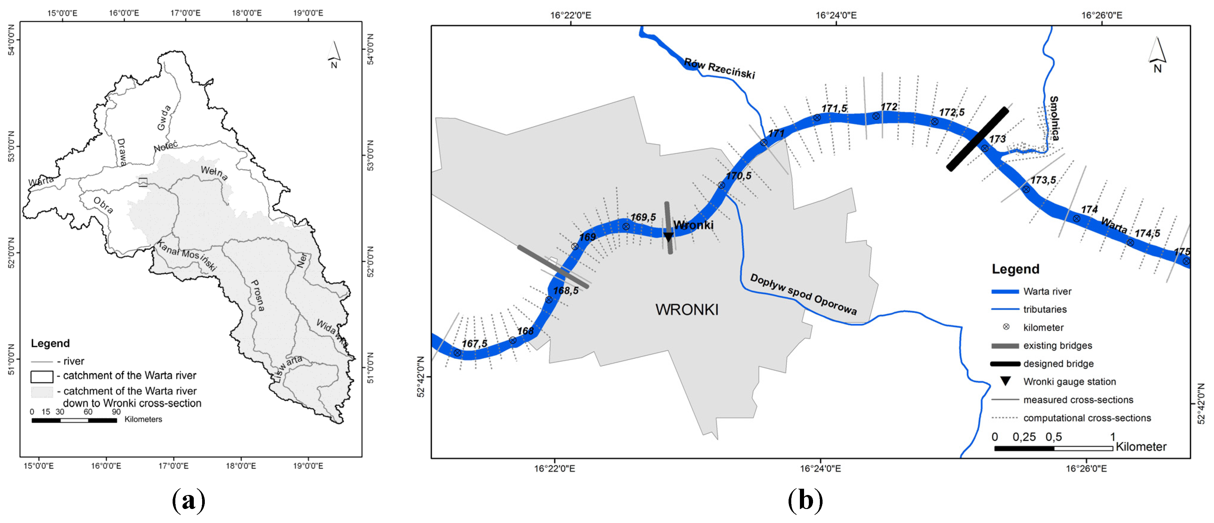
In this study, the field measurements and model simulations are focused on assessment of the impact of a bridge planned to be constructed on the Warta River on the flood hazard in the nearby area. The bridge is a part of the Wronki bypass road. Its expected location is km 172 + 900 of the Warta River.
The Warta River is one of the largest rivers in Poland. It is the third longest river in Poland, with a total length of 808.2 km and the fourth largest river according to the watershed area, which equals to 54,480 km
2. The Warta River begins in the Krakow-Czestochowa Uplands at the altitude of 380 m above sea level (a.s.l) and is a tributary of the Oder River. The rivers meet at the altitude of 12 m a.s.l. The water levels are measured regularly at 25 gauge stations along the Warta River. The gauge stations are under control of the Institute of Meteorology and Water Management (in Polish.
Instytut Meteorologii i Gospodarki Wodnej—IMGW). The observations are also made at the Wronki gauge station located in km 169 + 850 of the Warta River. The catchment area is about 30,661 km
2 in size. This is about 56% of the total catchment area. The catchment area equals 30,569 km
2 in the section, where the designed bridge is to be located.
Figure 1a presents the catchment area of the Warta River. The area of catchment for the Wronki gauge station is marked in grey. The early spring floods supplied with molten snow are the most frequent in the catchment of the Warta River. The summer rain floods are less frequent and they impact local areas. The characteristic feature of the Warta floods is a rather slow routing of the flood wave. However, the inundation may be kept for relatively long periods with quite high maximum stages.
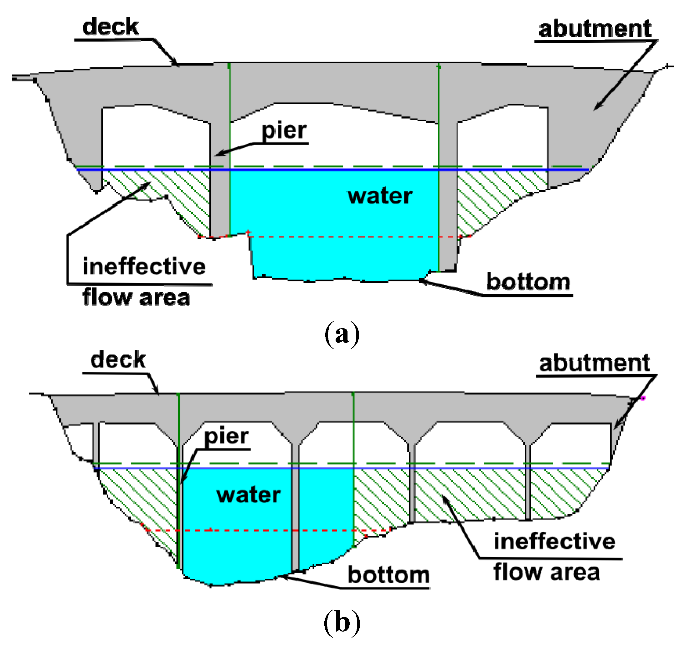
There are two bridges in the analyzed river section. The location of the bridges is presented in
Figure 1b. The bridges are shown in
Figure 2. The first one (
Figure 2a) is a railway bridge located downstream. The second one (
Figure 2b) is a road bridge located in the center of the Wronki town. This bridge links the left and right sides of the town of Wronki. The impact of the bridges on the hydraulic conditions in the Warta River is expected to be crucial. Hence, both bridges have to be properly taken into account in the computational model.
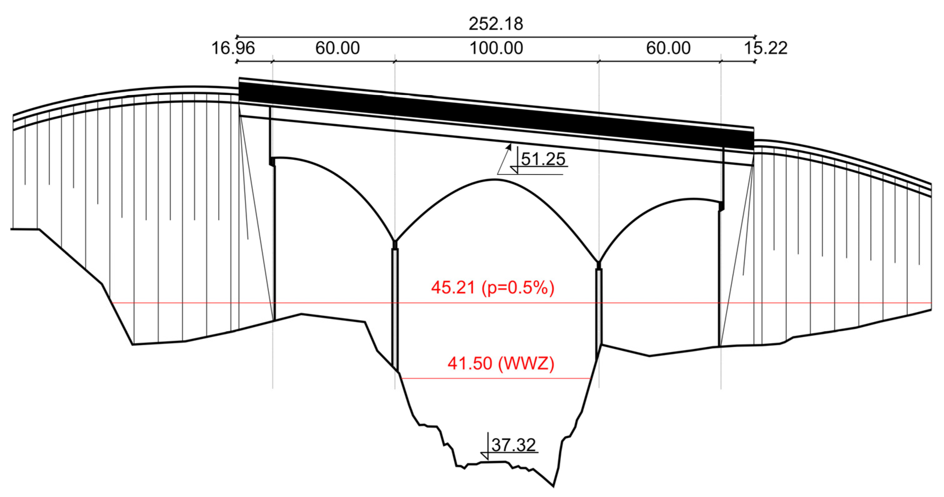
There were two variants of the bridge designed, with three and four spans. The total width of the spans were 220 and 270 m, respectively. Taking into account geological and economical requirements with topographic conditions, the first variant, presented in
Figure 3, was chosen. There are three spans with the widths 60, 100, and 60 m. The height of the bridge is 13.93 m above the river bottom at the highest point. Hence, the difference between water and the bridge ceiling is 9.75 m for admissible sailing conditions denoted as WWŻ (in Polish:
Wielka Woda Żeglowana = in English: High Navigable Water) in
Figure 3. Another water surface presented in
Figure 3 is 200-year flood. In this case the difference between water and the ceiling is 6.04 m.
Figure 1.
The location of the analyzed Warta River section (a); and distribution of the measured and computational cross-sections (b).
Figure 1.
The location of the analyzed Warta River section (a); and distribution of the measured and computational cross-sections (b).
Figure 2.
The existing bridges located in the town of Wronki: (
a) railroad bridge in km 168 + 773 (downstream); (
b) road bridge in km 169 + 871 (upstream) [
8].
Figure 2.
The existing bridges located in the town of Wronki: (
a) railroad bridge in km 168 + 773 (downstream); (
b) road bridge in km 169 + 871 (upstream) [
8].
It is easily seen that the problem presented here is very typical. In general, there is a number of bridges and other structures necessary to be taken into account in road construction. Hence, the methodology presented below on the basis of a single bridge may be considered as a more general approach to the problem of flood hazard analysis and updating of flood hazard maps.
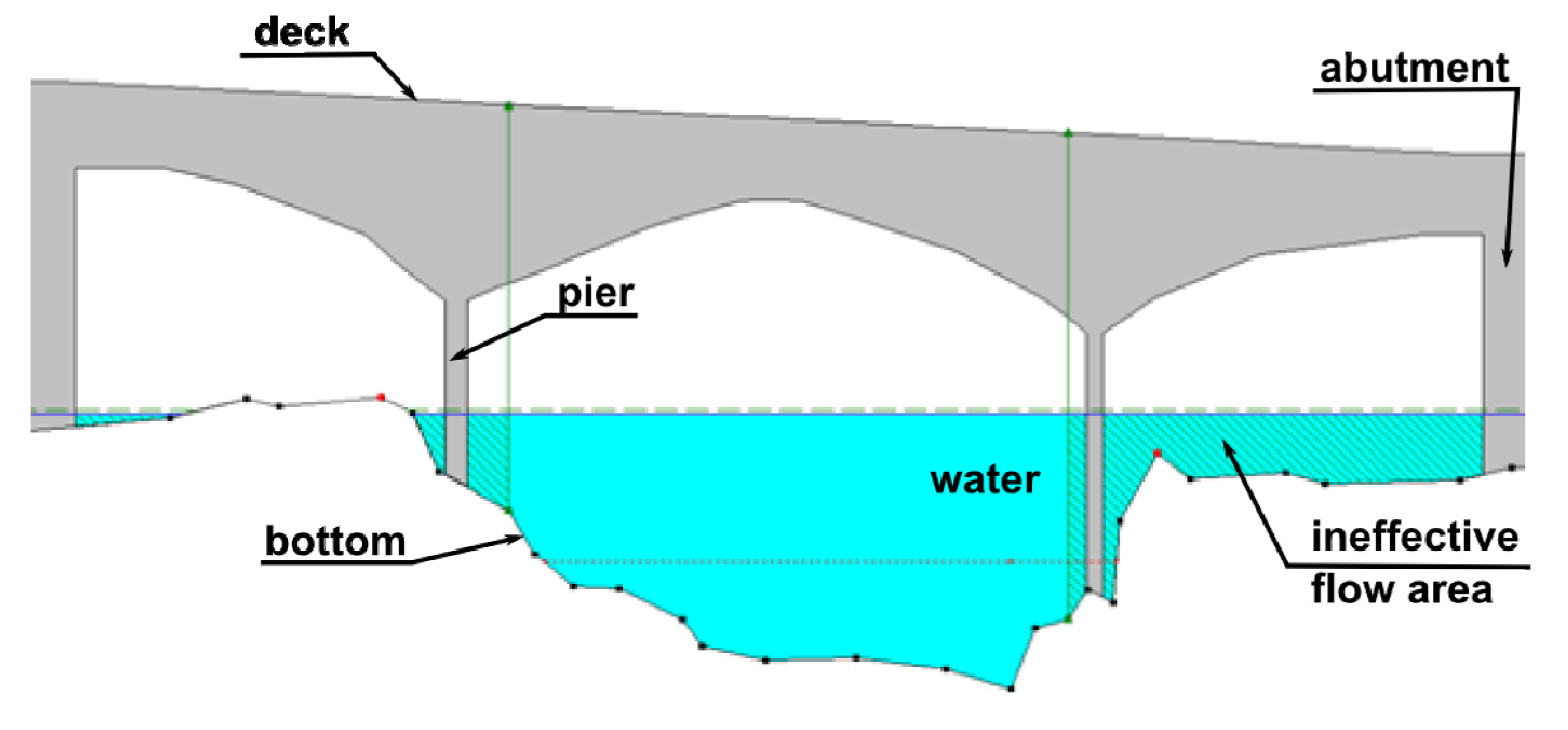
Figure 3.
The chosen variant of the designed bridge at km 172 + 913 with upstream cross-section. The scheme without scale. All sizes and elevations are given in meters.
Figure 3.
The chosen variant of the designed bridge at km 172 + 913 with upstream cross-section. The scheme without scale. All sizes and elevations are given in meters.
3. Materials and Methods
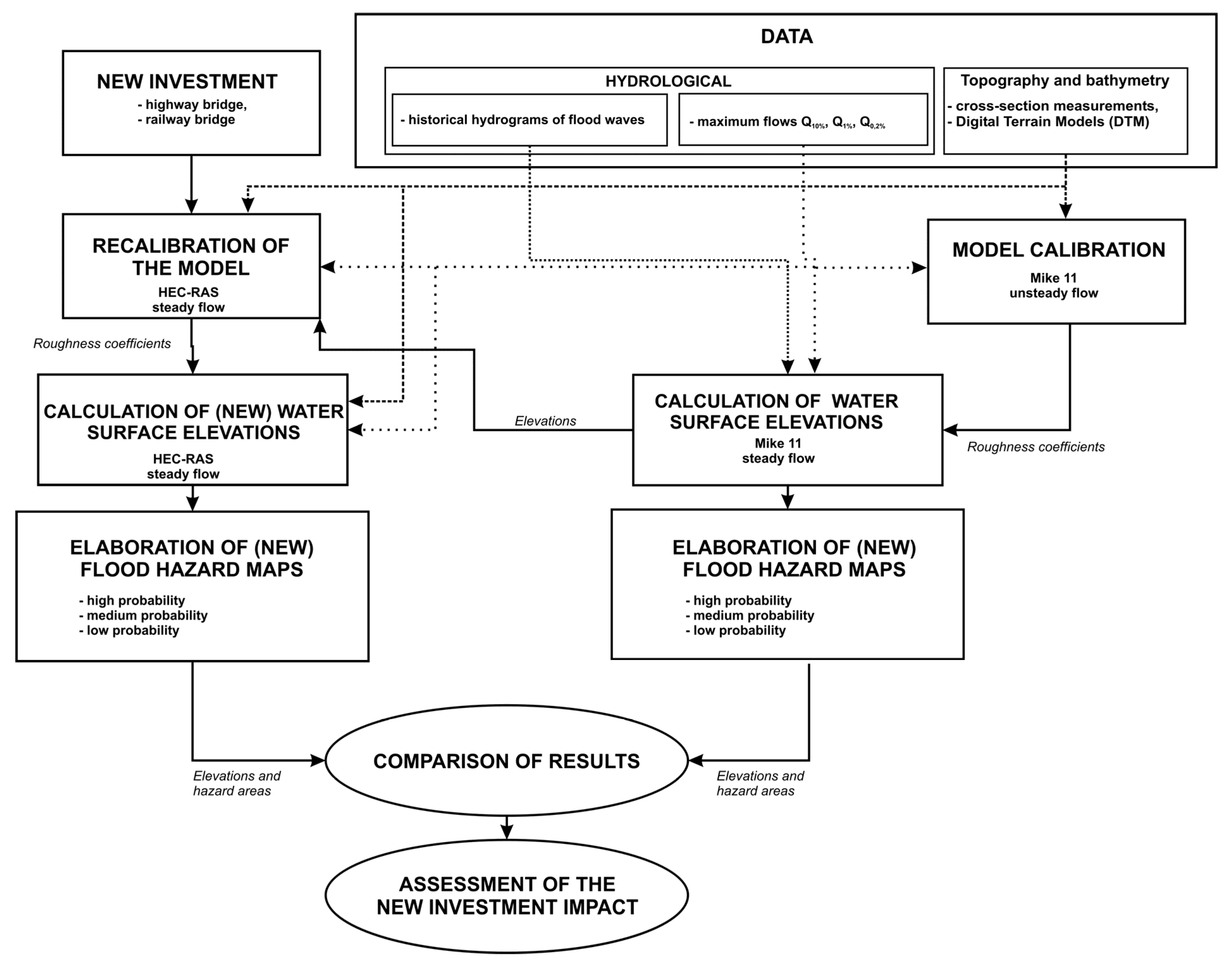
In order to assess the potential impact of the bridge planned to be constructed on the flood hazard, simulations were made in the same way as in the ISOK project. The main idea of the methodology implemented here is presented in
Figure 4 The relatively simple passage of data and results in the ISOK project is presented on the righthand side of the scheme. All the data collected are used in the model configuration and calibration. The software used for 1D calculations in the ISOK project is MIKE11 [
9]. Then, the calibrated model is used for determination of water surface profiles for particular flows. In ISOK the flows chosen are Q
10%, Q
1%, and Q
0.2% [
6]. Their values are as follows: 560.0 m
3·s
−1, 928.0 m
3·s
−1, and 1211.0 m
3·s
−1, respectively. The next step is to export of the water surface elevations to ArcGIS 10 [
10]. The flood hazard maps are generated on the basis of Digital Terrain Model (DTM) and calculated elevations. These maps show the spatial range of inundation and distribution of depths. The depths are divided into four groups. These are (a) 0.0–0.5 m; (b) 0.5–2.0 m; (c) 2.0–4.0 m; and (d) above 4.0 m [
6].
The lefthand side of the scheme in
Figure 4 presents the steps of the methodology implemented here. In this study the HEC-RAS software is used [
11]. This model differs slightly from MIKE11, but the main principle is the same. Both programs are numerical implementations of mass and momentum balance principles written in the form of St. Venant equations [
11,
12,
13,
14,
15]. These equations may be simplified to a single Bernoulli equation for steady flow [
11,
12,
13,
14,
15]. Then, the algorithm is based on the simple marching scheme, computing water elevation step-by-step. In subcritical flow regimes the computations are performed from downstream to upstream [
11]. The approach presented satisfies the first principle mentioned in the Introduction. The computations are physically-based. Additionally, the theoretical background of HEC-RAS and MIKE11 is almost the same. Hence, the second principle is not violated.
The model prepared by means of HEC-RAS software is composed of 26 standard cross-sections. The total length of the reach is over 7500 m. The average distance between cross-sections is about 40 m. The cross-sections are imported from the HEC-GeoRAS toolbox implemented in ArcGIS. This toolbox is described below. Each cross-section consists of the main channel, as well as left and right floodplains. In the standard model there are also two bridges located in the town of Wronki (
Figure 2). The bridges inserted into the computational model in HEC-RAS are presented in
Figure 5. The basis for bridge setups are measurements made by the IMGW team in the framework of the ISOK project. In both cases the standard approach implemented in HEC-RAS is used. The basic relationship used is the energy equation. In steady flow computations, it permits the determination of headwater elevation on the basis of discharge and tailwater level. Hence, the marching structure of the computational algorithm is not violated.
Figure 4.
Methodological scheme explaining the steps in the assessment of the impact of a new bridge on the flood hazard.
Figure 4.
Methodological scheme explaining the steps in the assessment of the impact of a new bridge on the flood hazard.
The next step of the model preparation is recalibration. This means that the new hydraulic model is configured in such a way that it gives the same results as the model used in the ISOK project. There is a basic assumption that the results of the ISOK project available are obtained with properly set and calibrated MIKE11. Hence, this model and its results fit flow process characteristics in the analyzed river reach well enough to consider this model as a proper representation of the modeled process. It suggests that calibration of another model on the basis of results should give us a model reconstruction of the flow process. When there is a lack of access to observations and the MIKE11 model, the presented approach is the only solution. In addition, such an approach satisfies the second principle specified in the Introduction. The implemented method is consistent with the one previously used in the ISOK project.
After recalibration of the model, the new bridge is inserted into the hydraulic model. The new water surface profiles are generated, and the new flood hazard maps are prepared. Finally, the results are compared and the impact is assessed. The details of the methodology are discussed below.
Standard Digital Terrain Model (DTM) is applied to reconstruct the topographic shape of the valley. The DTM is prepared on the basis of the airborne laser scanning LIDAR. The DTM is provided by the Geodesic and Cartographic Documentation Center (in Polish.
Centralny Ośrodek Dokumentacji Geodezyjnej i Kartograficznej—CODGIK) [
16]. The spatial resolution of the applied DTM is 1 m × 1 m. The altitude accuracy is 0.15 m for urbanized areas and 0.3 m for forests.
Figure 5.
HEC-RAS representation of modeled bridges located in Wronki: (a) railroad bridge in km 168 + 773 (downstream); and (b) road bridge in km 169 + 871 (upstream).
Figure 5.
HEC-RAS representation of modeled bridges located in Wronki: (a) railroad bridge in km 168 + 773 (downstream); and (b) road bridge in km 169 + 871 (upstream).
The DTM taken from CODGiK databases does not include bathymetric data of the riverbed. Before preprocessing of hydraulic modeling data it is necessary to obtain a proper reconstruction of river bottom elevations and link them with the basic DTM. For this purpose, the data obtained from the ISOK project are used [
6]. The ISOK project (in Polish.
Informatyczny System Osłony Kraju przed nadzwyczajnymi zagrożeniami) was realized by IMGW [
4]. The main element of the project is the implementation of the EU Flood Directive [
3] in Poland. The database prepared as one of the project products includes such elements as direct measurements of river cross-sections, bridges, and several hydraulic structures. The ISOK database stores 16 standard cross-sections and two bridges along the analyzed Warta River section (
Figure 1B). On the basis of these cross-sections the DTM for the riverbed is prepared. The DTMs of the riverbed and river valley are combined according to the methodology proposed by Merwade
et al. [
17]. All necessary data processing was performed by means of ArcGIS 10 tools [
10].
The final DTM is used as the basis for preparation of the river and floodplain geometry with the use of the HEC-GeoRAS toolbox [
18] implemented in ArcGIS 10. The HEC-RAS version 4.1.0 is used for hydraulic simulations [
11]. Both HEC-GeoRAS and HEC-RAS are freeware models developed by the Hydrologic Engineering Center, a part of the U.S. Army Corps of Engineers. The basic modules of HEC-RAS are one dimensional models permitting calculations for steady and unsteady flows of the river and for the floodplain flow. Only the steady flow algorithm based on the standard Bernoulli’s equation is applied in this study. The fundamental equation is adopted for the cases with broad floodplains [
11]. The procedure is completed with proper formulae for bridge modeling. The method used in HEC-RAS is the standard marching technique [
11]. This software also includes advanced tools for data preprocessing. The geometries of the river with floodplains are the basis of the river system modeling. The bridges and hydraulic structures are easily reconstructed. The software also enables visualization and analysis of results. The results may be also exported in GIS format and then analyzed by means of ArcGIS.
The model has been calibrated before use as a tool for assessment of the bridge impact on the flood risk. The basis of the calibration is the correct choice of roughness coefficients so that the results obtained would agree with the water elevations determined in the ISOK project. There are nine points along the analyzed Warta River section for which the ISOK results are available. The necessary values of maximum flows are obtained from the same database. The proper roughness coefficients are chosen simultaneously for all maximum flows, namely Q
10%, Q
1%, and Q
0.2%. However, the marching solution [
11] technique enables handling of roughness coefficients from reach-to-reach, where “reach” means all the computational cross-sections between points for which the ISOK results are available. The tools “Observed Data” and “Run Multiple Plans” [
19] available in HEC-RAS are used for such procedures.
The verification is performed on dependent variables and, finally, the model quality is assessed on the basis of commonly used statistical measures. The chosen measures are the correlation coefficient (
R), special correlation coefficient (
RS), and total square error (
STE) [
20]. The first of them is defined as:
where
N is the number of compared values,
Ho is water surface elevation read off from flood hazard maps available in the ISOK website, and
Hm is the water surface elevation calculated by HEC-RAS in the same locations for which
Ho values were determined. Both measured and calculated water surface elevations are expressed in meters m a.s.l.
The special correlation coefficient (RS) is calculated as follows:
The total square error (STE) is determined on the basis of the definition shown below:
The values calculated for our analyses are compared with the classification of model quality given by Sarma
et al. [
21]. Since the classification is important for assessment of the results, it is shown in
Table 1.
Table 1.
Criteria of model quality.
Table 1.
Criteria of model quality.
| Evaluation Criterion | Accordance Measure |
|---|
| Excellent | Very Good | Good | Pretty | Bad |
|---|
| R | >0.95 | 0.95–0.80 | 0.80–0.70 | 0.70–0.60 | ≤0.60 |
| RS | >0.95 | 0.95–0.80 | 0.80–0.70 | 0.70–0.60 | ≤0.60 |
| STE | <3 | 3–6 | 6–10 | 10–25 | ≥25 |
After the model calibration, the additional cross-sections are inserted. This operation is performed in order to prepare a model for the assessment of the bridge impact on the flood hazard. These are the cross-sections at the bridge location as well as 1 km upstream and downstream of the structure. Finally, the proper construction of the investigated bridge is configured in HEC-RAS. The method applied is the same as that described above for the existing bridges.
Figure 6 presents the designed bridge construction inserted in HEC-RAS. The water surface for
Q1% flow is also presented there.
Figure 6.
HEC-RAS representation of the designed bridge located at km 172 + 913.
Figure 6.
HEC-RAS representation of the designed bridge located at km 172 + 913.
The flood hazard maps obtained are compared with the results of the ISOK project [
4]. The tools available in ArcGIS software enabled the creation of differential maps. The last results present the impact of the planned bridge on the range of flood hazard zones, as well as water surface profile, in the 500-year; 100-year, and 10-year flood conditions. The applied procedure of assessment of the impact of a new investment on the flood hazard is presented in
Figure 4. The methodological scheme shown there may be applied for assessment of any investment impact on the flood hazard.
4. Results and Discussion
The selected results of recalibration are presented in
Table 2. The calibrated roughness coefficients for the main channel are presented in column 2. Their values vary between 0.030 (km 171 + 000) and 0.065 (km 168 + 808, 169 + 909). These values seems to be acceptable. The roughness coefficients obtained for floodplain are higher. Although, the minimum is 0.040 (km 171 + 000), the maximum is 0.11 (km 168 + 808). The results can be explained by intensive growth of floodplain vegetation observed there. Taking into account the obtained roughness coefficients, the result of our computations agree well with those of the ISOK project. The columns denoted
Q10,
Q1, and
Q0.2, show the differences between the model results and results of the project. The results for km 167 + 343 are not presented because at this cross-section the downstream boundary condition is imposed. Hence, the agreement of the model and ISOK results is perfect for this cross-section. The minimum obtained difference is 0.01 cm. The maximum is greater and equals 8.02. The agreement between the model results and the ISOK project data is uniform. The best fit is obtained for the crucial
Q1 flow. The average difference is 2.16 cm in this case.
Table 2.
Selected results of model recalibration.
Table 2.
Selected results of model recalibration.
| km | Roughness | Difference in Water Surface Elevation (cm) |
|---|
| Main Channel | Floodplain | Q10 | Q1 | Q0.2 |
|---|
| 174 + 912 | 0.042 | 0.08 | 6.84 | 3.38 | 8.02 |
| 173 + 452 | 0.042 | 0.08 | 5.68 | 2.15 | 4.13 |
| 172 + 051 | 0.035 | 0.05 | 1.53 | 3.71 | 1.91 |
| 171 + 000 | 0.030 | 0.04 | 0.65 | 0.7 | 4.22 |
| 169 + 909 | 0.065 | 0.08 | 2.59 | 1.54 | 0.31 |
| 169 + 871 | existing road bridge in Wronki |
| 169 + 811 | 0.035 | 0.05 | 0.01 | 0.4 | 1.57 |
| 168 + 808 | 0.065 | 0.11 | 2.25 | 2.25 | 1.29 |
| 168 + 773 | existing railway bridge in Wronki |
| 168 + 702 | 0.035 | 0.08 | 0.63 | 3.11 | 4.13 |
| 167 + 343 | 0.035 | 0.08 | – | – | – |
| average | 2.52 | 2.16 | 3.20 |
| min | 0.01 | 0.4 | 0.31 |
| max | 6.84 | 3.71 | 8.02 |
It has to be noted that the accuracy of the DTM used is 30 cm for forest areas and 15 cm for other areas. These values have to be taken as the measure of data uncertainty. Hence, the calibration provided very accurate results and greater accuracy should not be expected.
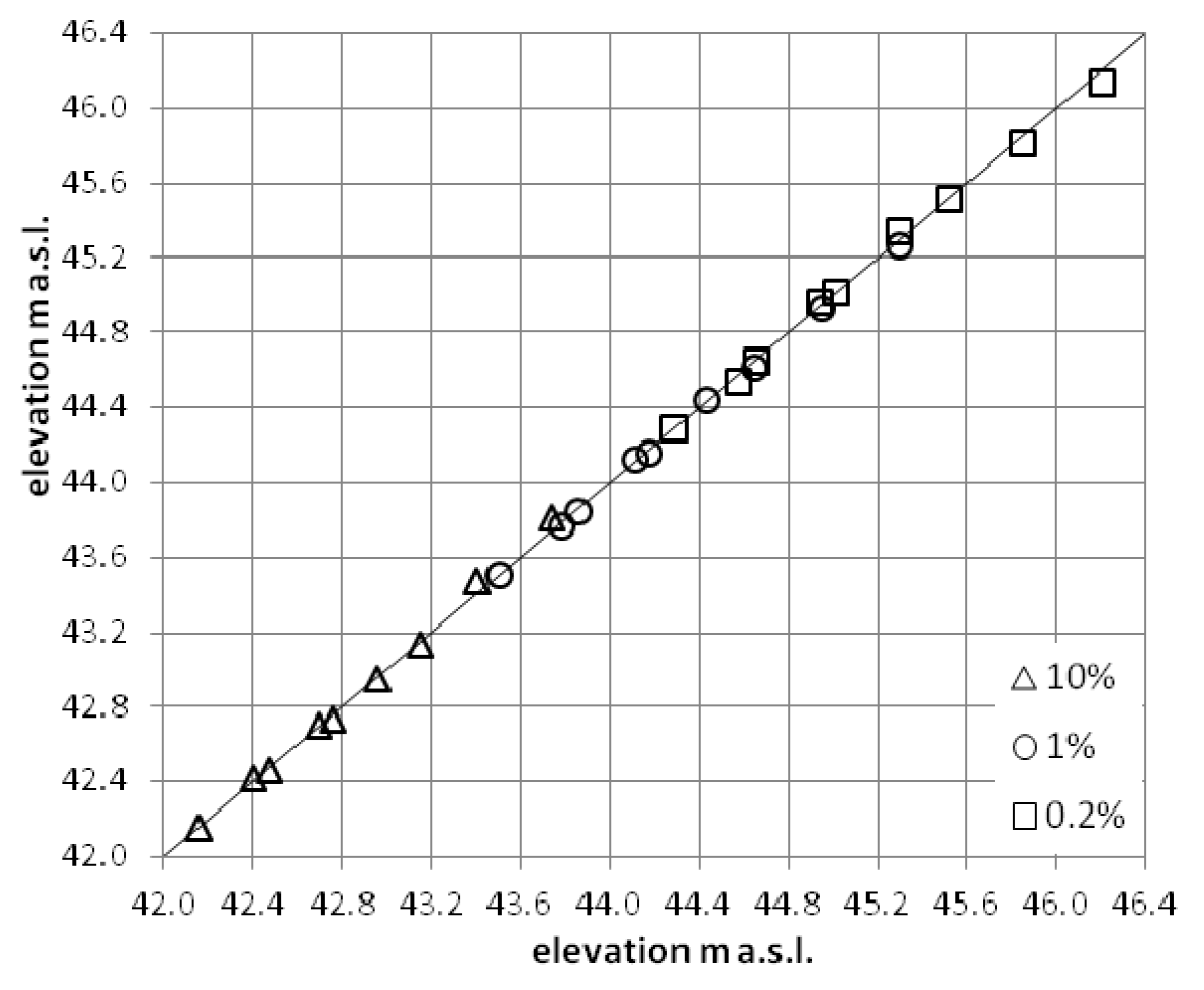
The quality of verification is illustrated in
Figure 7. This graph shows the relationship between water surface elevation determined in the ISOK project (horizontal axis) and those calculated by the implemented model (vertical axis). The straight line represents the equivalence between the ISOK project results and the results provided by the model we used. Hence, it represents a perfect fit of the model predictions to the observations. The calibration results for flows
Q10%,
Q1%, and
Q0.2% are denoted as crosses, dots, and stars, respectively. The model results are located very close to the line of the perfect fit. This means the model results are strongly correlated with the ISOK values. The agreement described in terms of previously-defined coefficients is as follows: correlation coefficient
R = 0.999, special correlation coefficient
RS = 1, and total square error
STE = 0.1%. According to the classification of models given by Sarma
et al. [
21] presented in
Table 1, the quality of the model is excellent.
For the assessment of model calibration quality, the differences between water surface elevations in the ISOK cross-sections are calculated. The values of absolute differences vary between 0.0 and 8.0 cm and the average is 2.3 cm. For the maximum flows
Q10%,
Q1%, and
Q0.2% the average absolute differences are equal to 2.2, 1.9, and 2.8 cm, respectively. During the calibration the specific roughness coefficients are assigned to the main channel and floodplains. The values obtained for the main channel vary from 0.030 to 0.065. Hence, they are in the range given by Van Te Chow [
12] for large rivers of width over 30 m with regular cross-sections. Higher values are assigned for floodplains. They are kept in the range of 0.040 to 0.110. The floodplains are mainly covered with high grass, wicker, and single bushes. In some places trees grow. Hence, such a structure of vegetation on floodplains explains higher values of roughness coefficients. In general, the values of calibrated roughness are reasonable and they are kept in the range of physically-interpreted values.
The assessment of the bridge impact on flood hazard is based on a comparison of water elevations. as well as average flow velocities for the two cases: before and after the bridge is configured in the model. The computations show that the planned bridge is able to increase the water levels along the distance 2 km upstream. The average increase in the water surface elevations for the maximum flows Q10%, Q1%, and Q0.2% is 0.4, 3.6, and 6.7 cm. The estimated changes in the average flow velocities are small and do not exceed 2 cm/s. However, the decrease in the velocity upstream of the bridge may be the reason for additional deposition of sediments there. Such effects may lead to additional increases in water levels, which may alter the conclusions drawn from our simulations.
Figure 7.
Quality of the model calibration.
Figure 7.
Quality of the model calibration.
Supposedly, the presented results do not properly visualize the spatial changes in the water surface and depth, so the results are also shown in the form of flood hazard maps, as well as longitudinal water surface profiles.
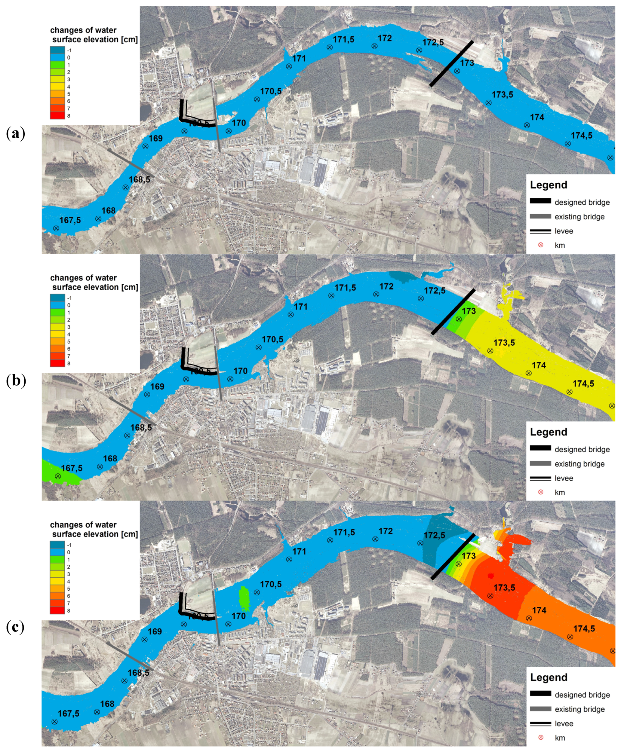
The assessment of the bridge impact on the flood hazard in the Warta River valley is presented in the form of differential maps of water surface elevation (
Figure 8). The flood hazard areas differ slightly from those presented in the ISOK project. The differences are of about 3% in the analyzed valley of the Warta River. The reason for such small changes is the topography of the valley. It is rather narrow with relatively steep hillsides.
In
Figure 8 the increments of water surface elevations are black, but decrements are presented as white areas. The analysis of water surface before and after the bridge construction shows that the changes are zero for the flow
Q10% (
Figure 8a). The flow
Q10% is kept in the banks, which explains such an effect. The maps show that only maximum flows
Q1% and
Q0.2% cause some changes between current hydraulic conditions and the estimated conditions after the bridge is built (
Figure 8b,c). In the attached figures the increase in the water surface level is clearly seen in the area upstream of the new bridge. Additionally, the increase in water surface in the Warta River also causes an increase in the water surface elevations in its right tributary, the Smolnica River. However, the potential changes in water levels do not exceed 8 cm. As it is indicated above, in the Materials and Methods, the vertical accuracy of the DTM used for non-forest areas is 0.15 m. In actuality, the potential bridge impact is lower than the uncertainty of the data applied.
Figure 8.
Calculated changes in water surface elevations for maximum flows Q10% (a); Q1% (b) and Q0.2% (c).
Figure 8.
Calculated changes in water surface elevations for maximum flows Q10% (a); Q1% (b) and Q0.2% (c).
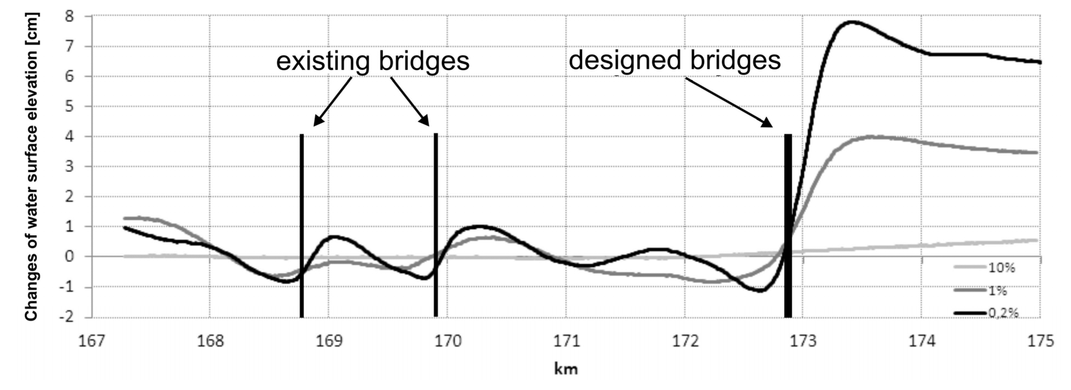
On the basis of the differential maps prepared, the longitudinal profile representing changes in the water surface elevation for the whole valley of the Warta River reach is obtained (
Figure 9). In the figure the changes in water surface profiles for the flows
Q10%,
Q1%, and
Q0.2% are denoted as light grey, regular grey, and dark grey lines, respectively. In the profile the impact of the bridge on the water levels is clearly visible. The greatest changes occur upstream of the bridge. There, the increase in water surface elevation is observed for the flows
Q1% and
Q0.2%. In some cross-sections, the water surface levels decrease on the opposite side, downstream of the bridge. This decrease is about 1 cm in comparison with water surface levels before the bridge construction. The other bridges also influence the hydraulic conditions in this part of the river section. The influence of the existing bridges may also be observed as small increase in the water levels upstream of each structure. However, this impact is rather small and does not cause an increase in water levels greater than 1 cm.
Figure 9.
The longitudinal profile of water elevations changes for maximum flows Q10%, Q1%, and Q0.2%.
Figure 9.
The longitudinal profile of water elevations changes for maximum flows Q10%, Q1%, and Q0.2%.
5. Conclusions
The inspiration for the presented paper was the implementation of EU Flood Directive in Poland. Huge losses related to floods that have been suffered over the last few years have imposed additional regulations in the area of flood management. The existence of legally-proved flood hazard maps also changes the rules for future actions in the catchments and construction related in any way to rivers. The direct purpose of the study described in this paper is the development of a methodology for the assessment of the impact of new investments on the flood hazard. Our analyses were made for a system of the Warta River section located near the town of Wronki. It is a typical example of flood threat and flood hazard assessment in Poland.
For the purpose of the paper, the assessment of impact of the new bridge planned is done according to the rules introduced in the EU Flood Directive. The water surface profiles and inundation areas for maximum flows Q10%, Q1%, and Q0.2% are the basis for presented comparisons. The whole procedure consists of three main steps: (1) data collection and model configuration; (2) generation of new results and post-processing; and (3) comparison of previous and current results and assessment of the impact. The most time consuming is the first step, including DTM preparation and model recalibration. The results of this step gave an excellent fitting of the proposed model predictions to the results of the model used in the ISOK project. This agreement validates the data obtained with our model. The second step includes calculations of water surface elevations, preparation of water surface profiles, and generation of flood inundation maps. In the stage of comparison, the differences between previous and current results are analyzed.
The approach presented here enabled the evaluation of the range of new bridge impacts, the form of those impacts, as well as the intensity of the impacts. The range is shown in the maps and water surface profiles and it is understood as the length of the river section where the differences between previous and current results are observed. For the Warta River section studied, the range is spread upstream of the bridge as well as downstream, but the form of the impact is different. In the upstream of the bridge, the new investment increases the water stages. The consequences are higher depths and more extended inundation areas. In the downstream, the water surface elevations are decreased and resulting effects are the opposite. The depths are lower and the spread of inundation is smaller. Such results were expected, but the quantitative assessment required detailed computations described here.
The procedure presented in the paper guarantees the compatibility of the results with the procedures of the ISOK project and requirements of the EU Flood Directive. The most important elements are the preparation of the DTM, including the riverbed and recalibration of the model. The purpose of the first step is to reconstruct the topography of water flows in and beyond the river channel. The second step is focused on getting similarity in the results of the simulation of the physical phenomena. These two elements determine the coherence of the previous and current results and they also determine the validity of comparisons and drawn conclusions.
The problem presented here has become very common since the EU Flood Directive and flood hazard maps were implemented in Poland. The number of the planned investments is high, as mentioned in the Introduction. Their relation to flood hazard assessment is obvious in many cases. The flood hazard maps would be out of date in the not too distant future without reliable procedures for their update or very important investments would be stopped. Hence, the procedure presented here is aimed at breaking some impasse, which would appear after implementation of the EU Flood Directive. The advantage of the method described is its independence of tools used for development of flood hazard maps in the ISOK project, while maintaining full compatibility with the results determined in this project.


